Hidden Markov Models: Probabilistic Sequence Labeling for NLP

Sequence labeling tasks like POS tagging require more than just looking up each word in a dictionary. The word "bank" could be a noun (a financial institution) or a verb (to bank on something). The word "flies" could be a noun (the insects) or a verb (the action of flying). Context determines the correct label, and that context often spans multiple words in a sequence.

Hidden Markov Models (HMMs) provide a principled probabilistic framework for sequence labeling. An HMM models two interacting processes: a hidden sequence of states (the tags you want to predict) and an observable sequence of outputs (the words you can see). The model learns statistical patterns about how states transition to each other and how each state generates observations. Given a new sentence, the HMM uses these learned patterns to infer the most likely hidden sequence.

This chapter covers HMM components and their probabilistic foundations. You'll learn how to estimate HMM parameters from annotated data, understand the key assumptions that make HMMs tractable, and implement a working POS tagger. We'll also examine where HMMs succeed and where they fall short, setting up the motivation for more advanced models like Conditional Random Fields.

An HMM defines a joint probability distribution over two sequences: a hidden state sequence and an observable output sequence. In POS tagging, the hidden states are the part-of-speech tags, and the observations are the words.

The model has five components:

• States ($S$): A finite set of hidden states. For POS tagging, these are the tags like NN, VB, DT, JJ.
• Observations ($V$): A finite vocabulary of observable symbols. These are the words in your corpus.
• Initial probabilities ($\pi$): The probability of starting in each state. For sentences, this captures which tags typically begin sentences.
• Transition probabilities ($A$): The probability of moving from one state to another. This captures tag-to-tag patterns like "determiners are often followed by nouns."
• Emission probabilities ($B$): The probability of generating each observation from each state. This captures which words are associated with which tags.

Let's define these components mathematically. For a state sequence $s_1, s_2, \ldots, s_n$ and observation sequence $o_1, o_2, \ldots, o_n$, we define three probability distributions.

The initial probability captures how likely each state is to appear at the start of a sequence:

where $\pi_i$ is the probability that the first state in the sequence is state $i$.

The transition probability captures how states follow one another:

where:

• $a_{ij}$: the probability of transitioning from state $i$ to state $j$
• $s_t$: the state at position $t$ in the sequence
• $s_{t-1}$: the state at the previous position

The emission probability captures how each state generates observations:

where:

• $b_i(o)$: the probability of observing symbol $o$ when in state $i$
• $o_t$: the observation at position $t$
• $s_t$: the hidden state at position $t$

These three distributions fully characterize an HMM's behavior. The initial probabilities determine how sequences start, transitions determine how states evolve, and emissions determine what we observe.

To make these concepts concrete, let's build a toy HMM for POS tagging. We'll use just three states (determiner, noun, verb) and five words, which is enough to see the key patterns while keeping the numbers tractable.

The transition matrix encodes grammatical patterns. Determiners (DT) are followed by nouns (NN) with probability 0.8, capturing the common English pattern "the dog" or "a cat." The emission matrix encodes lexical associations. The word "the" is emitted by DT with probability 0.9, while "runs" is emitted by VB with probability 0.5.

HMMs make two key independence assumptions that simplify computation. These assumptions trade off modeling power for tractability.

The first assumption is the Markov property: the probability of transitioning to a state depends only on the current state, not on the full history.

where:

• $s_t$: the state at position $t$ (what we want to predict)
• $s_1, s_2, \ldots, s_{t-1}$: the full history of previous states
• $s_{t-1}$: only the immediately preceding state

The equation states that knowing the entire history provides no additional information beyond knowing just the previous state. For POS tagging, this means the probability of a tag depends only on the previous tag, not on tags from earlier in the sentence. If the previous tag is DT (determiner), the probability of NN (noun) is the same regardless of what came before the determiner.

This is a strong assumption. Consider "the old old man" versus "the very old man." After seeing "old" once, the probability of another adjective might differ from seeing "old" for the first time. A first-order HMM cannot capture this distinction.

The second assumption is output independence: the probability of an observation depends only on the current state, not on other observations or states.

where:

• $o_t$: the observation at position $t$ (the word we see)
• $s_1, \ldots, s_n$: all hidden states in the sequence
• $o_1, \ldots, o_{t-1}, o_{t+1}, \ldots, o_n$: all other observations (past and future words)
• $s_t$: only the current hidden state

The equation states that the probability of emitting a particular word depends solely on the current tag, not on any surrounding context. For POS tagging, this means the word "bank" has the same emission probability from the NN state regardless of surrounding words. The model cannot use the context "river bank" to increase the probability of the noun interpretation.

These assumptions enable efficient algorithms for inference and learning. The Viterbi algorithm (covered in the next chapter) finds the most likely state sequence in $O(n \cdot |S|^2)$ time, where $n$ is the sequence length and $|S|$ is the number of states. Without these assumptions, exact inference would require exponential time.

Given an HMM, how do we compute the probability of a particular observation sequence and state sequence? The joint probability factors according to the HMM structure, exploiting the independence assumptions to decompose a complex probability into simple terms.

For an observation sequence $O = o_1, o_2, \ldots, o_n$ and state sequence $S = s_1, s_2, \ldots, s_n$, the joint probability is:

where:

• $P(O, S)$: the joint probability of observing sequence $O$ while the hidden states follow sequence $S$
• $P(s_1)$: the initial probability of starting in state $s_1$, denoted $\pi_{s_1}$
• $P(o_1 \,|\, s_1)$: the emission probability of the first observation given the first state, denoted $b_{s_1}(o_1)$
• $\prod_{t=2}^{n}$: the product over all positions from 2 to $n$
• $P(s_t \,|\, s_{t-1})$: the transition probability from state $s_{t-1}$ to state $s_t$, denoted $a_{s_{t-1}, s_t}$
• $P(o_t \,|\, s_t)$: the emission probability of observation $o_t$ from state $s_t$, denoted $b_{s_t}(o_t)$

The formula captures the generative story of an HMM: start in some state (with probability $\pi$), emit the first word (with probability $b$), then repeatedly transition to a new state (with probability $a$) and emit the next word (with probability $b$).

Let's compute this for a concrete example: the sentence "the dog runs" with tags "DT NN VB." We'll trace through each step of the computation, showing how the probabilities multiply together to give the joint probability of this particular word-tag pairing.

The joint probability is quite small because we're multiplying many probabilities together. For longer sequences, these products become vanishingly small, leading to numerical underflow. In practice, we work in log space, converting multiplications to additions.

An HMM is only useful if we can learn its parameters from data. For POS tagging, we have access to annotated corpora where each word is labeled with its correct tag. This is supervised learning, and parameter estimation is straightforward: we count occurrences and normalize.

The maximum likelihood estimates for HMM parameters are simple frequency ratios derived from counting occurrences in the training data.

For initial probabilities, we count how often each state starts a sequence:

where:

• $\hat{\pi}_i$: the estimated probability of starting in state $i$
• $\text{count}(s_1 = i)$: the number of sequences that begin with state $i$
• $\text{count}(\text{sequences})$: the total number of sequences in the training data

For transition probabilities, we count how often state $j$ follows state $i$:

where:

• $\hat{a}_{ij}$: the estimated probability of transitioning from state $i$ to state $j$
• $\text{count}(s_{t-1} = i, s_t = j)$: the number of times state $i$ is immediately followed by state $j$
• $\text{count}(s_{t-1} = i)$: the total number of times state $i$ appears (except at sequence end)

For emission probabilities, we count how often state $i$ emits observation $o$:

where:

• $\hat{b}_i(o)$: the estimated probability of emitting observation $o$ from state $i$
• $\text{count}(s_t = i, o_t = o)$: the number of times state $i$ emits observation $o$
• $\text{count}(s_t = i)$: the total number of times state $i$ appears

In words: the initial probability of state $i$ is the fraction of sequences that start with $i$. The transition probability from $i$ to $j$ is the fraction of times $i$ is followed by $j$. The emission probability of $o$ from $i$ is the fraction of times state $i$ emits $o$.

Let's implement this with NLTK's tagged corpora. The Brown corpus contains over 57,000 sentences with POS tags, giving us enough data to estimate reliable probabilities. We'll use the Universal tagset, which maps the fine-grained Brown tags to 17 coarse categories for cleaner patterns.

The estimated parameters reveal clear patterns. The initial probability distribution shows which tags typically begin sentences in English:

: Initial state probabilities estimated from the Brown corpus. Determiners (DET), nouns (NOUN), and pronouns (PRON) dominate sentence beginnings, reflecting common English patterns. {#tbl-initial-probs}

Determiners, nouns, and pronouns dominate sentence beginnings, together accounting for over 75% of sentence starts.

Another revealing view is how emission probabilities vary across tags for ambiguous words. The word "run" can be a noun ("a morning run") or a verb ("I run daily"). Let's see how the learned emission probabilities capture this ambiguity:

: Emission probabilities for ambiguous words across POS tags. "Time" shows moderate noun vs. verb ambiguity. "Run" is more strongly verbal. "Set" has substantial probability from both noun and verb tags, reflecting its high ambiguity in English. {#tbl-emission-ambiguity}

The table reveals that "time" has higher emission probability from NOUN than VERB, but both are non-zero, reflecting genuine ambiguity. These patterns form the statistical backbone of HMM-based tagging.

A critical challenge emerges when we encounter words not seen during training. If a word $o$ never appeared with tag $i$, then $\hat{b}_i(o) = 0$. When we multiply by zero, the entire sequence probability becomes zero, making it impossible to tag sentences containing unknown words.

Smoothing techniques address this problem. The simplest approach is add-one (Laplace) smoothing: add a small count to every word-tag combination before normalizing.

where:

• $\hat{b}_i(o)$: the smoothed emission probability of observation $o$ from state $i$
• $\text{count}(s_t = i, o_t = o)$: the number of times state $i$ emits observation $o$ (zero for unseen combinations)
• $\text{count}(s_t = i)$: the total number of times state $i$ appears
• $|V|$: the vocabulary size (number of unique observations)

The numerator adds 1 to every count, ensuring no probability is ever zero. The denominator adds $|V|$ to compensate, keeping the probabilities properly normalized (summing to 1). This ensures every word has a non-zero probability from every tag, though the probability is very small for unseen combinations.

With smoothing, unseen words get a small but non-zero probability from each tag. This allows the HMM to tag sentences containing new words by relying on transition probabilities to disambiguate.

Now let's build a complete HMM POS tagger. Given a sentence, we want to find the most likely tag sequence. This is the decoding problem:

where:

• $\hat{S}$: the optimal (most likely) state sequence
• $\arg\max_S$: "the value of $S$ that maximizes" the following expression
• $P(S \,|\, O)$: the posterior probability of state sequence $S$ given observations $O$
• $P(O, S)$: the joint probability of observations and states

The second equality follows from Bayes' rule: $P(S \,|\, O) = P(O, S) / P(O)$. Since $P(O)$ is constant for a given observation sequence (it doesn't depend on which state sequence we're evaluating), maximizing the posterior is equivalent to maximizing the joint probability.

A naive approach would enumerate all possible tag sequences, compute their joint probabilities, and return the maximum. But with $|S|$ tags and $n$ words, there are $|S|^n$ possible sequences. For 12 tags and a 20-word sentence, that's over 3.8 quadrillion possibilities.

The Viterbi algorithm solves this efficiently in $O(n \cdot |S|^2)$ time using dynamic programming. We'll cover Viterbi in detail in the next chapter. For now, let's implement a simplified greedy decoder that selects the locally best tag at each position.

Greedy decoding works as follows: for the first word, we pick the tag that maximizes $\pi_i \cdot b_i(o_1)$. For each subsequent word, we pick the tag that maximizes $a_{prev, i} \cdot b_i(o_t)$ given the previous tag we chose. This is fast but can make mistakes when a locally optimal choice leads to a globally suboptimal sequence.

The greedy tagger works reasonably well for straightforward sentences but can make errors when local decisions conflict with global coherence. The sentence "The old man the boat" is a famous garden path sentence where "man" is actually a verb (meaning "to operate") and "old" is a noun phrase ("the elderly people"). Greedy decoding often misses such non-local dependencies because each decision only considers the immediately preceding tag.

The transition matrix is the heart of an HMM's syntactic knowledge. By visualizing it as a heatmap, we can see which tag sequences the model considers likely and which it considers rare. This provides insight into both the structure of English grammar and the quality of our learned model.

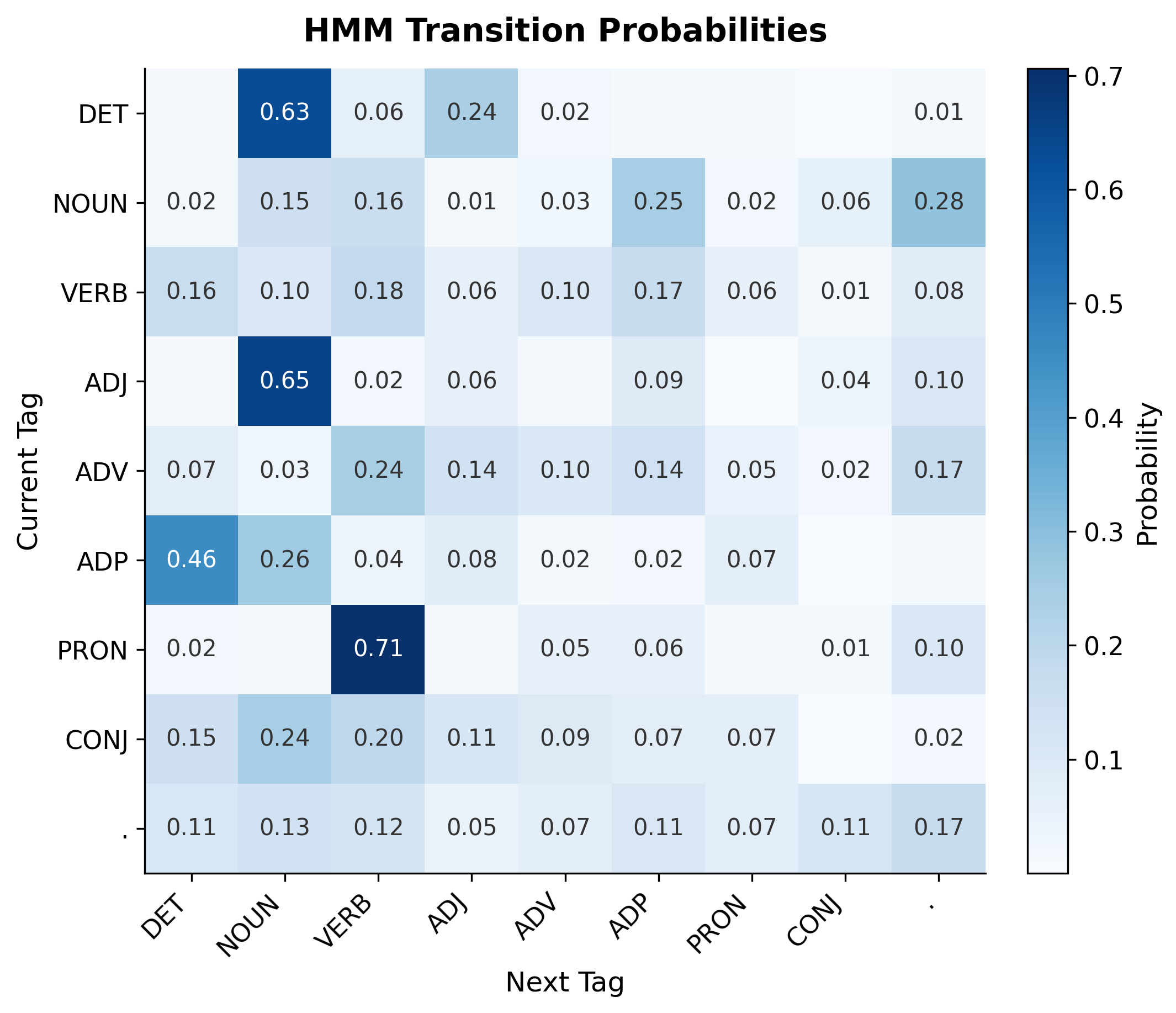
The transition matrix reveals clear syntactic patterns. Determiners (DET) have high transition probability to nouns (NOUN) and adjectives (ADJ). Nouns frequently transition to verbs (VERB) or punctuation. Prepositions (ADP) strongly predict nouns, reflecting prepositional phrase structure. These patterns are exactly what we'd expect from English grammar.

How well does our HMM tagger actually perform? To answer this rigorously, we need to evaluate on data the model hasn't seen during training. We'll split the Brown corpus into 90% training and 10% test, re-estimate all parameters on the training portion, and measure accuracy on the held-out test sentences.

We'll also track performance separately for known words (those seen during training) versus unknown words. This distinction matters because the model handles these cases very differently: known words have learned emission probabilities, while unknown words must rely entirely on transition patterns and smoothed probabilities.

: HMM tagger accuracy on the Brown corpus test set. The model achieves high accuracy on known words where emission probabilities provide strong signals. Unknown word accuracy drops substantially because the model must rely solely on transition probabilities and smoothed emissions. {#tbl-accuracy}

The accuracy gap between known and unknown words is striking. For known words, the model performs reasonably well because emission probabilities provide strong signals. For unknown words, the model must rely entirely on transition probabilities, which provide weaker disambiguation.

This evaluation uses greedy decoding, which makes locally optimal choices. The Viterbi algorithm (next chapter) finds the globally optimal sequence and typically improves accuracy by 2-5 percentage points, especially for difficult cases where local and global optima differ.

To understand how an HMM resolves ambiguity, let's trace through the complete probability computation for the classic ambiguous sentence "Time flies." This two-word sentence has two plausible interpretations, and both words can function as either nouns or verbs:

• "Time flies" could mean "Time passes quickly" (NOUN VERB)
• "Time flies" could mean "Measure how fast flies move" (VERB NOUN)

We'll compute the joint probability for each interpretation and see which one the HMM prefers. Since we're multiplying many small probabilities, we'll work in log space to avoid numerical underflow.

To understand why the HMM prefers NOUN VERB, let's decompose the log probability into its components: initial probability, emissions, and transitions.

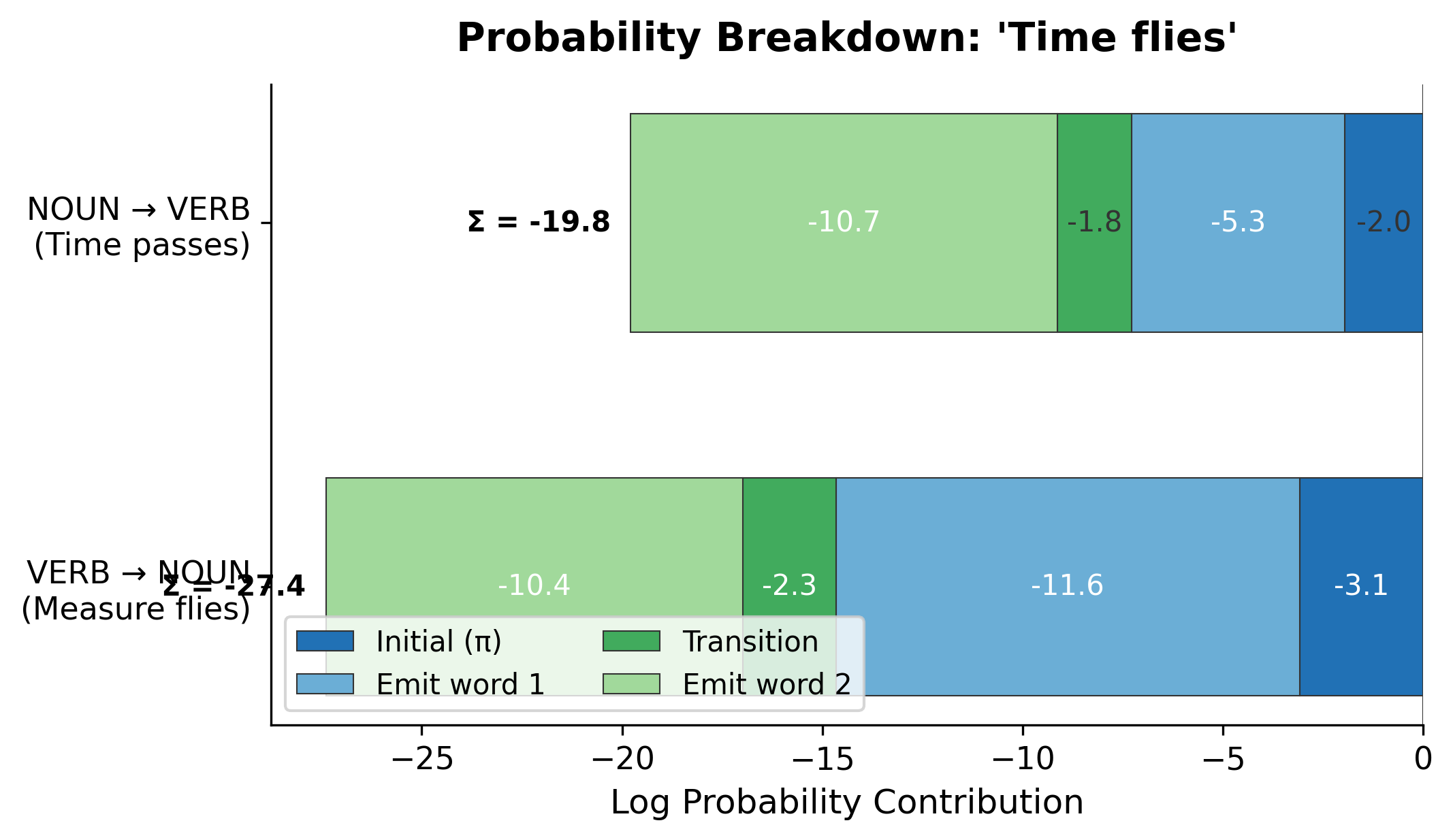
The HMM prefers "Time flies" as NOUN VERB. This makes sense: in the training data, sentences starting with nouns are more common than sentences starting with verbs, and noun-verb transitions are frequent. The emission probability of "time" from NOUN is also higher than from VERB, since "time" appears as a noun more often in general text.

This example illustrates how HMMs combine multiple sources of evidence: initial probabilities favor starting with nouns, transitions favor noun-verb patterns, and emissions favor "time" as a noun and "flies" as a verb.

HMMs were the dominant approach to sequence labeling from the 1980s through the early 2000s. They remain instructive for understanding probabilistic sequence models and provide a foundation for more advanced techniques.

The independence assumptions that make HMMs tractable also limit their power. The emission independence assumption is particularly restrictive: an HMM cannot condition on neighboring words when deciding what tag to emit. Consider the word "set." In "the set of numbers," it's a noun. In "set the table," it's a verb. An HMM can only use transition probabilities to disambiguate, ignoring the direct evidence from surrounding words like "the" before "set" or "table" after "set."

The Markov assumption also causes problems for long-distance dependencies. In "The dog that the cat chased runs," the verb "runs" must agree with "dog," but an HMM only sees the immediately preceding "chased." Higher-order HMMs (conditioning on two or three previous tags) help but create exponentially more parameters to estimate.

Unknown words present another challenge. With smoothing, unknown words get similar emission probabilities from all tags. The model must rely on transitions, but transition probabilities alone often can't disambiguate. Modern approaches use character-level features (suffixes like "-tion" suggest nouns, "-ly" suggests adverbs) or pretrained embeddings that generalize to unseen words.

Despite these limitations, HMMs achieved remarkable success and enabled practical NLP systems for the first time.

The Viterbi algorithm made efficient exact inference possible, allowing HMM taggers to process text at thousands of words per second. This efficiency was crucial for applying NLP to large document collections.

The forward-backward algorithm enabled unsupervised learning from raw text. You could train an HMM without any labeled data, discovering latent structure in the tag sequences. While unsupervised HMMs never matched supervised accuracy, they opened up possibilities for low-resource languages.

The probabilistic framework integrated naturally with other statistical models. HMM outputs could feed into named entity recognizers, parsers, and information extraction systems, with probabilities propagating through the pipeline.

HMMs also established the paradigm of sequence labeling as a structured prediction problem. The insight that labels depend on each other, not just on inputs, led to CRFs, neural sequence models, and eventually transformers with attention over the full sequence.

When implementing HMM-based taggers, several parameters affect model performance:

• Smoothing constant ($\alpha$): Controls how much probability mass is reserved for unseen word-tag combinations. Higher values (e.g., 1.0 for Laplace smoothing) give more weight to unseen events but dilute the learned emission probabilities. Lower values (e.g., 0.01) preserve learned distributions better but may underestimate rare events. Start with $\alpha = 1.0$ and tune based on unknown word accuracy.

• Tag set granularity: Finer tag sets (like Penn Treebank's 36 tags) capture more distinctions but require more training data and increase computational cost. Coarser sets (like Universal Dependencies' 17 tags) are easier to learn but lose information. Choose based on your downstream task requirements.

• Case normalization: Converting words to lowercase reduces vocabulary size and improves emission estimates for rare words, but loses capitalization signals that help identify proper nouns and sentence boundaries. The implementation above uses lowercase normalization.

• Unknown word handling: Beyond smoothing, you can improve unknown word accuracy by using morphological features (suffixes, prefixes, capitalization patterns) or by backing off to character-level models. The simple <UNK> token approach shown here provides a baseline.

Hidden Markov Models provide a probabilistic framework for sequence labeling. The model jointly models hidden state sequences (like POS tags) and observable output sequences (like words), learning statistical patterns for how states transition and what observations each state generates.

Key takeaways:

• HMM components include states, observations, initial probabilities, transition probabilities, and emission probabilities. These five elements fully specify the model
• The Markov assumption says each state depends only on the previous state, not the full history. This enables efficient algorithms but limits the model's ability to capture long-range dependencies
• The output independence assumption says each observation depends only on its current state. This prevents the model from using surrounding context to disambiguate emissions
• Maximum likelihood estimation learns parameters by counting occurrences in annotated data. Smoothing handles unseen word-tag pairs that would otherwise have zero probability
• Decoding finds the most likely state sequence given observations. Greedy decoding is fast but suboptimal; the Viterbi algorithm (next chapter) finds the globally optimal sequence efficiently
• HMM limitations include inability to use rich features, difficulty with long-distance dependencies, and weak handling of unknown words. These motivated the development of Conditional Random Fields and neural sequence models

HMMs exemplify a recurring theme in NLP: strong independence assumptions enable efficient algorithms, but real language violates these assumptions in important ways. The next chapter covers the Viterbi algorithm, which finds optimal sequences in $O(n \cdot |S|^2)$ time, and subsequent chapters introduce CRFs, which relax HMM's independence assumptions while preserving computational tractability.

Ready to test your understanding? Take this quick quiz to reinforce what you've learned about Hidden Markov Models and sequence labeling.