

Learn how Bahdanau attention solves the encoder-decoder bottleneck with dynamic context vectors, softmax alignment, and interpretable attention weights for sequence-to-sequence models.

This article is part of the free-to-read Language AI Handbook
Choose your expertise level to adjust how many terms are explained. Beginners see more tooltips, experts see fewer to maintain reading flow. Hover over underlined terms for instant definitions.
Bahdanau Attention
In the previous chapter, we developed an intuition for attention as a mechanism that allows models to selectively focus on different parts of the input when generating each output. We saw how attention acts as a soft lookup, assigning weights to encoder hidden states based on their relevance to the current decoding step. Now it's time to formalize this intuition into a concrete algorithm.
Bahdanau attention, introduced in the 2014 paper "Neural Machine Translation by Jointly Learning to Align and Translate," was the first attention mechanism to achieve broad success in sequence-to-sequence models. The key innovation was replacing the fixed context vector bottleneck with a dynamic, position-dependent context that changes at each decoder timestep. This change led to significant improvements in translation quality, especially for longer sentences.
The Alignment Problem
Before diving into the mathematics, let's understand the problem that Bahdanau attention solves. In a standard encoder-decoder architecture, the encoder processes the entire input sequence and compresses it into a single fixed-length vector. The decoder then generates the output sequence using only this compressed representation.
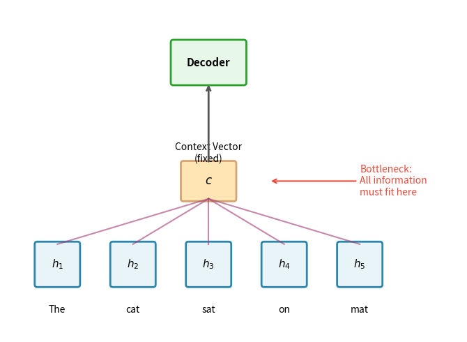
This bottleneck creates a fundamental problem: the context vector must somehow encode everything about the input that the decoder might need. For short sentences, this works reasonably well. But as input length increases, the fixed-size context vector becomes increasingly inadequate. Information gets lost, compressed, or muddled together.
The insight behind attention is that different parts of the output depend on different parts of the input. When translating "The cat sat on the mat" to French, generating "Le" depends mostly on "The," while generating "chat" depends mostly on "cat." Instead of forcing all this information through a single bottleneck, why not let the decoder directly access the relevant encoder states at each step?
In the context of attention, alignment refers to the correspondence between positions in the input and output sequences. Good alignment means the model correctly identifies which input positions are relevant for generating each output position. Bahdanau attention learns this alignment jointly with translation, rather than relying on external alignment tools.
The Attention Mechanism: From Intuition to Formulas
With the alignment problem clearly defined, we can now develop the mathematical machinery that Bahdanau attention uses to solve it. Our journey will take us through three interconnected concepts: computing relevance scores, converting those scores to probabilities, and aggregating information based on those probabilities. Each piece builds naturally on the previous one, culminating in a mechanism that allows the decoder to "look back" at exactly the right parts of the input at each generation step.
The Challenge of Measuring Relevance
Attention addresses a simple question: when the decoder is about to generate output token , how relevant is each encoder position to that decision? If we could answer this question with a single number for each encoder position, we'd have a way to rank and weight the encoder states.
But what should this "relevance score" capture? Consider translating "The cat sat on the mat" to French. When generating "chat" (cat), the decoder needs to know:
- What the decoder is currently looking for (encoded in its hidden state )
- What information each encoder position offers (encoded in hidden states )
The relevance of position depends on both of these: it's not just about what contains, but whether that content matches what the decoder currently needs. This suggests we need a function that takes both the decoder state and an encoder state as inputs and produces a scalar score.
The Additive Score Function
Bahdanau and colleagues designed a solution called the additive (or concatenative) alignment model. Rather than directly comparing the decoder and encoder states, which might have different dimensions and represent different types of information, they project both into a shared "alignment space" where comparison becomes meaningful.
The alignment score between decoder position and encoder position is computed as:
where:
- : the alignment score, a scalar indicating how relevant encoder position is for generating output
- : the decoder hidden state at the previous timestep, encoding what the decoder "knows" and "needs"
- : the encoder hidden state at position , encoding information about input token and its context
- : a learnable weight matrix that projects the decoder state into the alignment space
- : a learnable weight matrix that projects encoder states into the same alignment space
- : a learnable vector that reduces the combined representation to a scalar
- : the dimension of the alignment space (a hyperparameter, typically matching the hidden dimensions)
This formula might look complex at first glance, but it follows a clear logic. Let's trace through it step by step to understand why each component is necessary:
Step 1: Project into alignment space. The decoder state and encoder state live in potentially different vector spaces with different dimensions. Before we can meaningfully compare them, we need to transform them into a common representation. The matrices and learn these transformations during training:
- produces a -dimensional vector representing "what the decoder is looking for"
- produces a -dimensional vector representing "what encoder position offers"
Step 2: Combine additively. With both vectors in the same space, we add them element-wise: . This additive combination allows the model to detect when the decoder's query and the encoder's content are compatible. If certain dimensions align well (both positive or both negative), they reinforce each other; if they conflict, they cancel out.
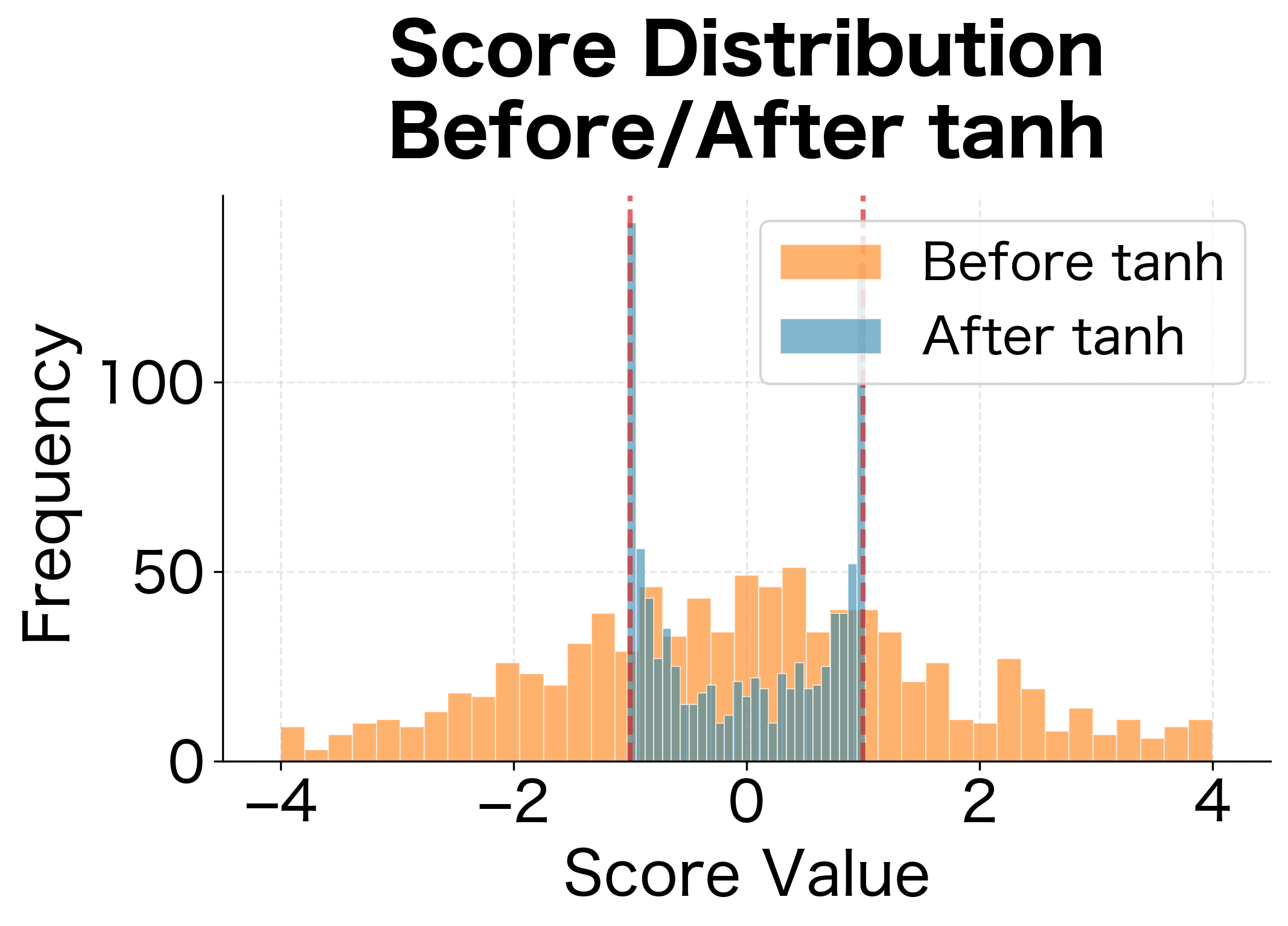
Step 3: Apply nonlinearity. The function serves two purposes. First, it bounds the values to , preventing any single dimension from dominating. Second, it introduces nonlinearity, enabling the model to learn complex, non-linear relationships between decoder queries and encoder contents. Without this nonlinearity, the entire alignment model would collapse to a simple linear function.
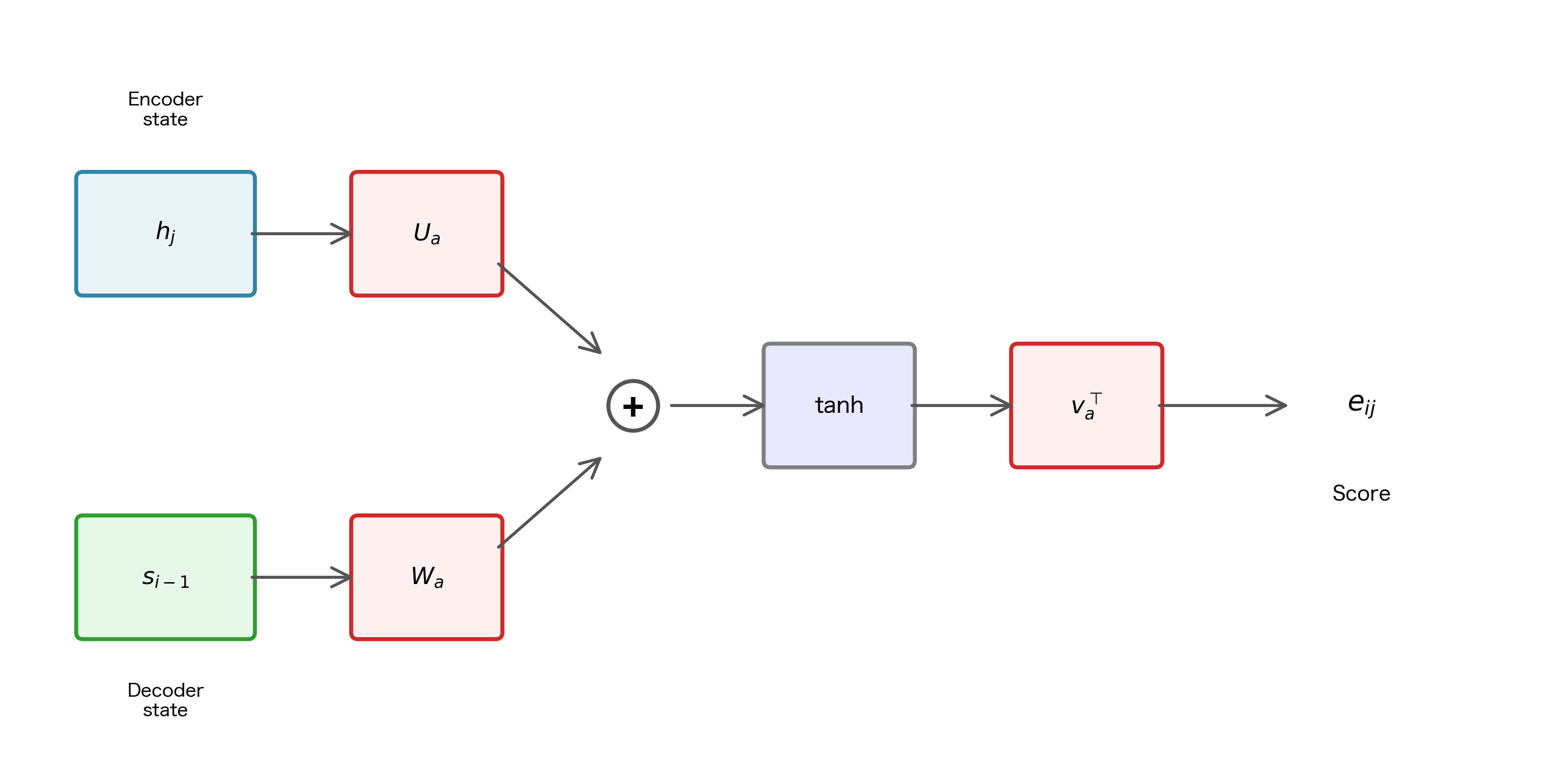
Step 4: Reduce to scalar. Finally, the dot product with compresses the -dimensional result into a single scalar score. The vector learns which dimensions of the alignment space are most important for determining relevance. Some dimensions might capture semantic similarity, others syntactic compatibility; learns to weight these appropriately.
Why "additive" rather than some other approach? Additive combination with separate projection matrices gives the model maximum flexibility. The decoder and encoder might have different hidden dimensions, and even if they're the same size, they encode different types of information. By learning separate projections and , the model can transform each representation into whatever form makes comparison most effective. Bahdanau and colleagues found this approach worked well in practice, and it became the foundation for subsequent attention mechanisms.
From Scores to Probabilities: The Softmax Transformation
We now have a way to compute alignment scores for each encoder position. But these raw scores can be any real number: positive, negative, or zero. To use them for weighting encoder states, we need to transform them into something more interpretable: a probability distribution over encoder positions.
This is where the softmax function enters the picture. Softmax takes a vector of arbitrary real numbers and converts it into a valid probability distribution where all values are positive and sum to 1:
where:
- : the attention weight for encoder position when generating output
- : the raw alignment score from our scoring function
- : the exponential function ()
- : the length of the source sequence
- : the normalizing constant that ensures weights sum to 1
The exponential function is the key to softmax's behavior. It has two essential properties that make it ideal for attention:
- Positivity: for all real , guaranteeing non-negative weights regardless of the input scores
- Monotonicity with amplification: larger scores produce exponentially larger values, which amplifies differences between scores
This second property is particularly important. Consider two scores: and . The difference looks modest, but after exponentiation, while , a 10x ratio. Softmax creates a "winner-take-most" dynamic where the highest-scoring positions dominate, while still allowing lower-scoring positions to contribute.
The attention weight has a clear interpretation: it represents the probability that encoder position contains the information most relevant for generating output token . When we compute attention, we're asking: "Given what the decoder currently needs, where in the input should it look?"
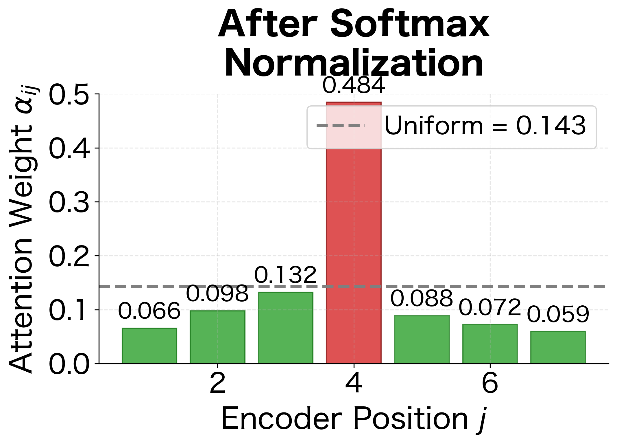
The visualization above shows this amplification in action. Position 4 has a raw score of 2.8, only about 2× higher than position 1's score of 0.8. But after softmax, position 4 receives about 4× the attention weight of position 1. This amplification helps the model make decisive choices about where to focus.
Beyond the mathematical properties, softmax has two important advantages for learning:
- Differentiability: Gradients flow smoothly through softmax, enabling end-to-end training with backpropagation.
- Soft selection: Unlike "hard" attention (which would pick exactly one position), soft attention maintains gradients to all positions, making optimization much easier.
The "softness" of attention can be controlled by scaling the scores before applying softmax. Dividing scores by a temperature parameter changes how sharply the attention focuses:
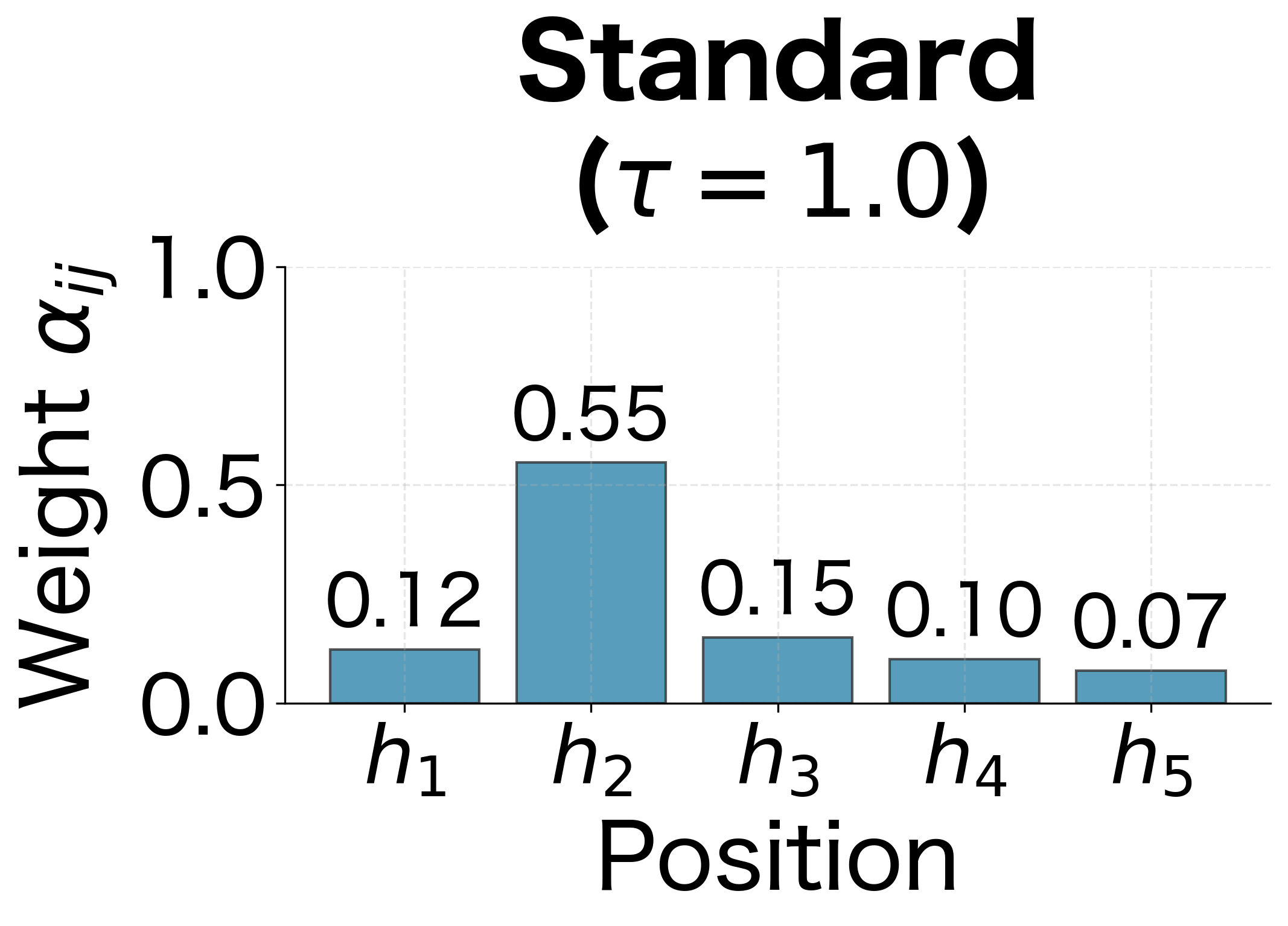
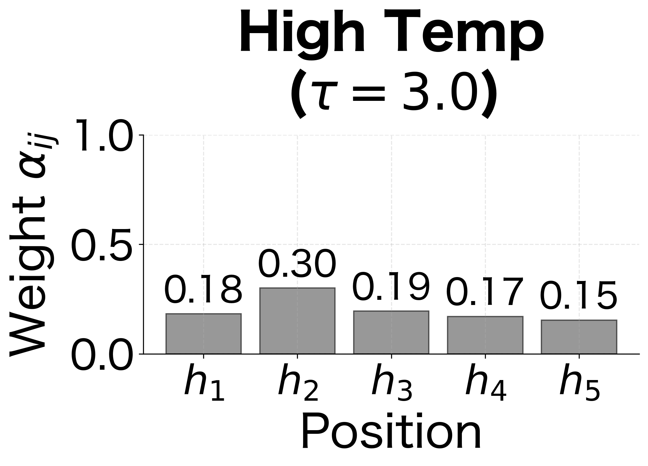
The entropy values in the figure quantify the "spread" of attention: lower entropy means more focused attention, higher entropy means more distributed. Standard Bahdanau attention uses , which provides a good balance between focusing on relevant positions and maintaining gradient flow to all positions during training.
The "sharpness" of the attention distribution depends on the magnitude of score differences. When scores are similar, attention spreads across many positions; when one score is much higher, attention concentrates sharply:
The entropy values quantify this difference: higher entropy indicates more spread-out attention, while lower entropy indicates more concentrated attention. A well-trained model learns to produce focused attention when one input position is clearly relevant (e.g., translating a content word) and spread attention when multiple positions contribute (e.g., translating a phrase that spans multiple source words).
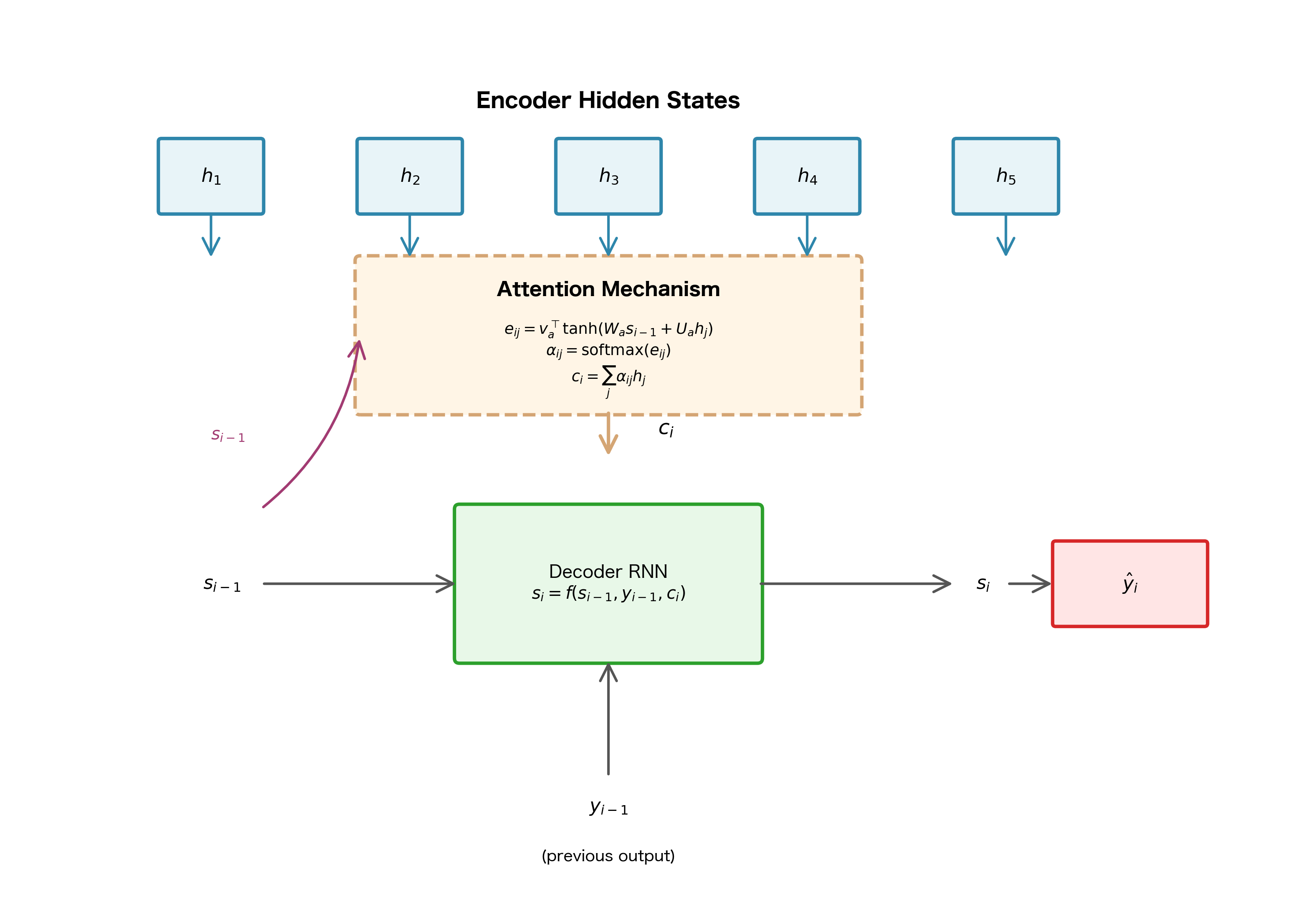
Aggregating Information: The Context Vector
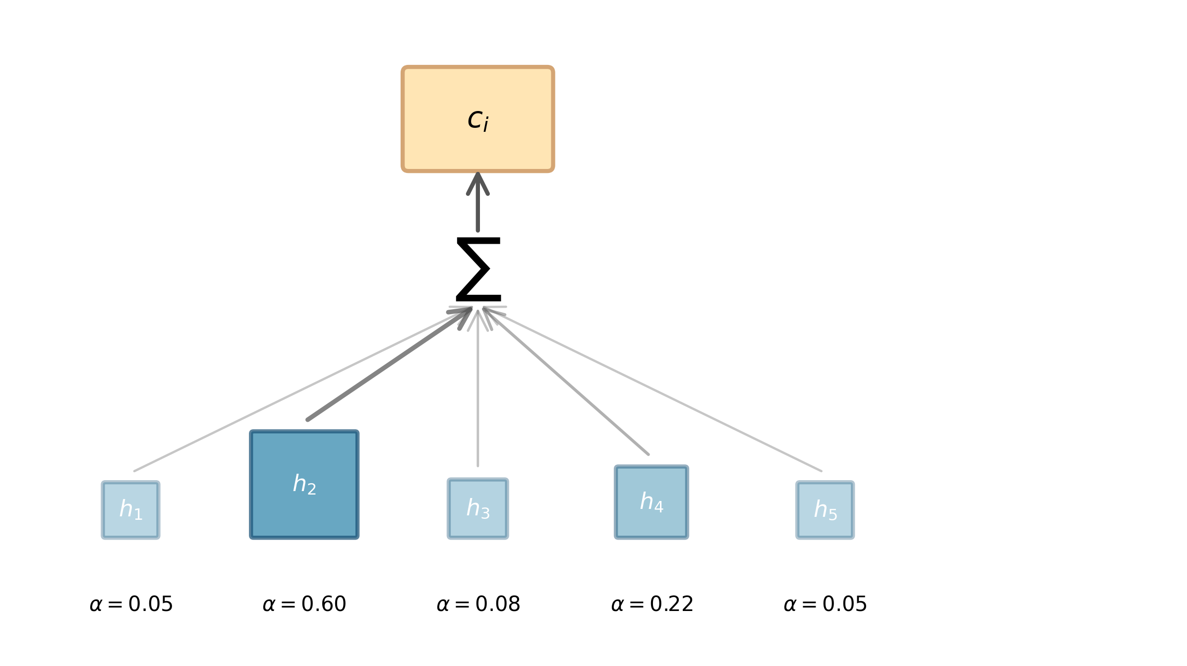
We've now computed attention weights that tell us how much the decoder should attend to each encoder position. The final step is to use these weights to create a single vector that summarizes the relevant information from the entire input sequence. This is the context vector.
The context vector for decoder position is simply a weighted sum of the encoder hidden states:
where:
- : the context vector, a -dimensional summary of the relevant input information
- : the attention weight for encoder position (how much to attend to that position)
- : the encoder hidden state at position
- : the length of the source sequence
This formula is simple, but its implications are significant. Because the attention weights sum to 1, the context vector is a convex combination of the encoder states. It lies somewhere "between" them in the vector space, closer to the states with higher weights.
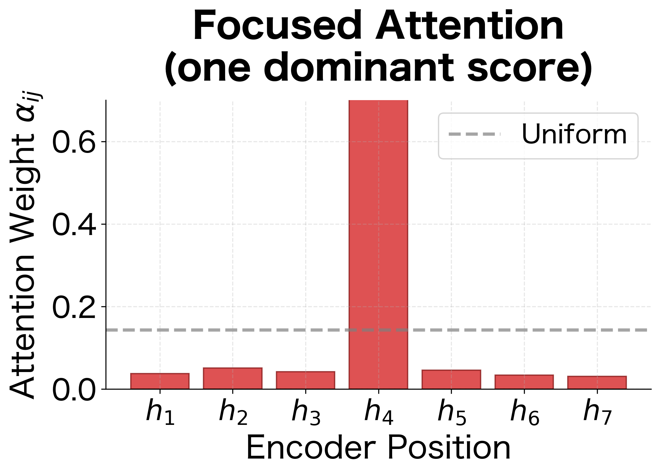
Consider what happens in different scenarios:
- Focused attention: If and all other weights are near zero, then . The context vector copies the encoder state at position 2.
- Distributed attention: If weights are spread across multiple positions, the context vector blends information from all of them. This is useful when the decoder needs information from multiple parts of the input.
- Uniform attention: If all weights are equal (), the context vector is the simple average of all encoder states, similar to a mean-pooling operation.
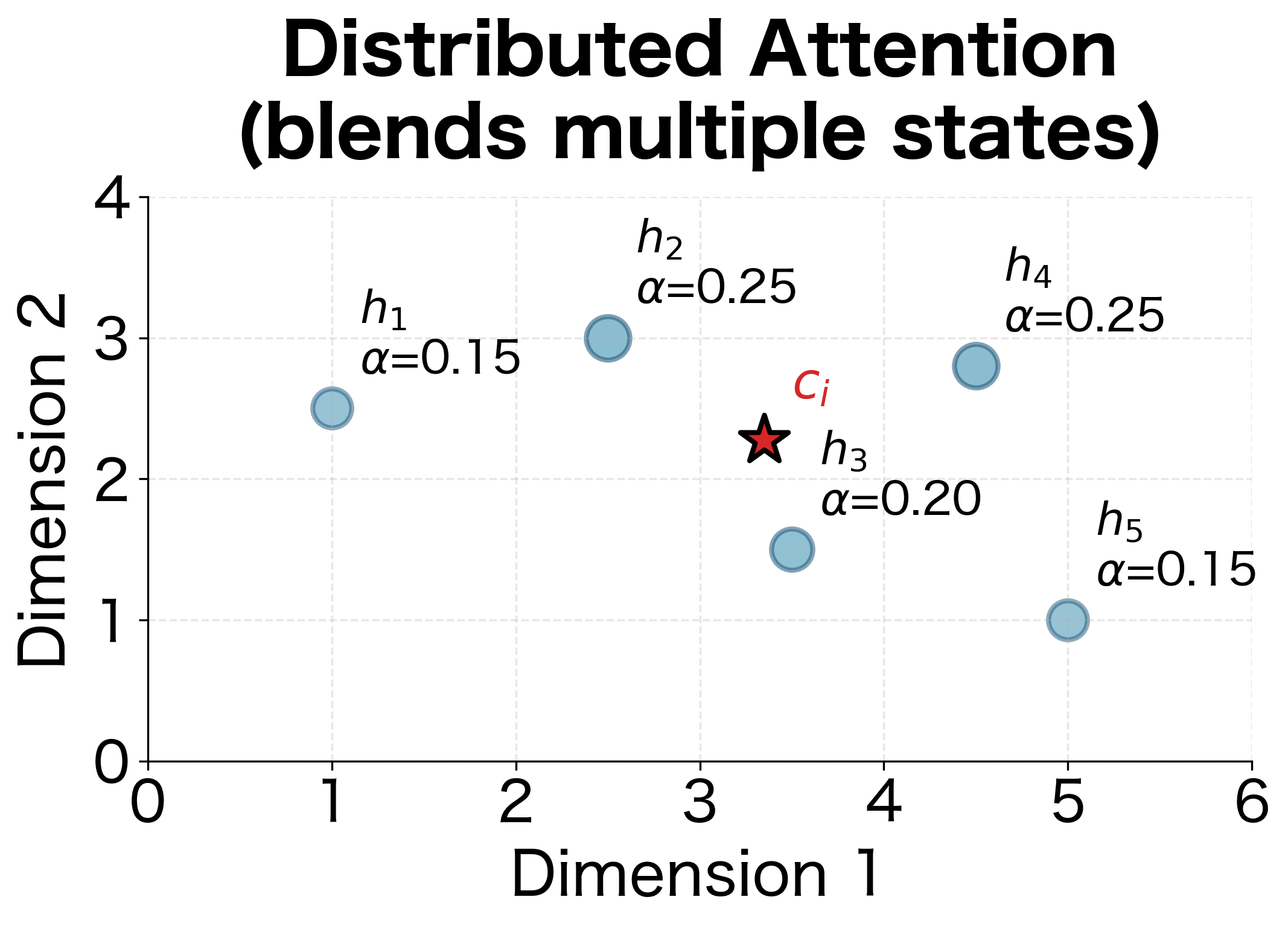
This geometric interpretation helps build intuition: the context vector "moves" through the encoder state space based on attention weights, getting pulled toward whichever states receive more attention. The model learns to position the context vector where it captures the most relevant information for the current generation step.
The key insight is that each decoder step gets its own context vector , computed fresh based on the current decoder state . This is the main improvement over standard encoder-decoder models: instead of forcing all information through a single fixed-size bottleneck, we dynamically select and aggregate the relevant parts of the input at each generation step.
Putting It All Together: The Complete Attention Mechanism
We've now developed all three components of Bahdanau attention:
- Scoring: measures relevance
- Normalization: converts scores to probabilities
- Aggregation: creates a weighted summary
But how does this attention mechanism integrate with the decoder RNN? The context vector contains a summary of the relevant input information, but the decoder also needs to know what it has generated so far and maintain its own internal state.
In Bahdanau's formulation, these three sources of information are combined by feeding them into the decoder RNN:
where:
- : the new decoder hidden state after processing step
- : the previous decoder hidden state (the decoder's "memory")
- : the embedding of the previous output token
- : the context vector from attention
- : a recurrent cell function (typically GRU or LSTM)
In practice, and are concatenated into a single vector of dimension before being fed to the RNN. This combines information about the previous prediction with the attention-weighted summary of the input.
The complete decoding process at step follows this sequence:
- Compute alignment scores: For each encoder position , calculate
- Normalize to attention weights: Apply softmax to get
- Compute context vector: Calculate
- Update decoder state: Compute
- Generate output: Predict the next token using (and often as well)
One subtle but important detail: attention is computed using the previous decoder state , not the current state . This makes sense because we need to know what the decoder is looking for before we can compute the context, and we need the context before we can update the decoder state.
A Worked Example: Attention in Action
The formulas we've developed might seem abstract, so let's ground them with a concrete numerical example. We'll trace through every step of the attention computation, watching the numbers flow through each transformation.
Imagine we're building a translation system for English to French. We're translating "I love cats" and have just generated "J'" (the French equivalent of "I"). Now we need to generate the next word, which should be "aime" (love). The question is: which part of the input should the decoder focus on?
For this example, we'll use deliberately small dimensions so we can see every number:
- Hidden dimension: 4 (real systems use 256-1024)
- Alignment dimension: 3
- Source sequence: 3 words ("I", "love", "cats")
Each encoder hidden state captures information about word and its surrounding context. The decoder state encodes what the decoder has generated so far and, implicitly, what it's looking for next. The weight matrices , , and vector would normally be learned during training; here we use fixed values for illustration.
Step 1: Project the Decoder State
The first step is to transform the decoder state into the alignment space. This projection happens once per decoder step and will be reused when comparing against each encoder position:
This 3-dimensional vector represents "what the decoder is looking for" in the alignment space. Think of it as a query that we'll compare against each encoder position.
Step 2: Compute Alignment Scores
Now we compute a score for each encoder position. For each position , we project into the alignment space, add it to the projected decoder state, apply tanh, and compute the final score with :
The scores reveal that position 2 ("love") has the highest alignment with what the decoder is looking for. This makes intuitive sense: to generate "aime" (the French word for love), the decoder should focus on the English word "love." Position 3 ("cats") has the lowest score, indicating it's least relevant for this particular generation step.
Step 3: Normalize with Softmax
Raw scores can be any real number, but we need probabilities. Softmax transforms these scores into a proper probability distribution:
Position 2 receives about 45% of the attention, while positions 1 and 3 receive roughly 28% and 27% respectively. Notice that even though position 2 had the highest score, the attention isn't completely focused on it. This "soft" attention allows the model to hedge its bets, pulling in information from multiple positions when useful. The weights sum to exactly 1.0, confirming we have a valid probability distribution.
Step 4: Compute the Context Vector
Finally, we use these attention weights to create a weighted combination of the encoder hidden states:
The context vector is a blend of all three encoder states, weighted by their relevance. It's closest to (the representation of "love") since that position received the highest attention weight, but it also incorporates information from the other positions. This context vector now gets fed into the decoder RNN along with the previous output embedding to generate the next token.
We can measure how the context vector relates to the encoder states using cosine similarity:
| Encoder State | Word | Attention Weight | Cosine Similarity |
|---|---|---|---|
| "I" | 0.28 | 0.404 | |
| "love" | 0.45 | 0.821 | |
| "cats" | 0.27 | 0.150 |
The similarity analysis confirms that the context vector is closest to the encoder state that received the highest attention weight. However, the context isn't identical to any single encoder state; it's a weighted blend that can capture information from multiple positions when needed.
This worked example illustrates the key insight of attention: instead of forcing the decoder to work with a single fixed representation of the entire input, we dynamically construct a context that's tailored to each generation step. When generating "aime," the context emphasizes "love"; when generating "chats" later, the context would shift to emphasize "cats."
From Theory to Code: Implementing Bahdanau Attention
Having traced through the mathematics by hand, let's now implement Bahdanau attention as a PyTorch module. The code will mirror the formulas exactly, making it easy to see how each mathematical operation translates to tensor operations.
The implementation follows our mathematical formulation exactly. Let's trace through the key operations:
- Projection layers:
W_a,U_a, andv_aare implemented asnn.Linearlayers without bias terms, matching our weight matrices - Broadcasting: When we add
decoder_proj.unsqueeze(1)toencoder_proj, PyTorch broadcasts the decoder projection across all sequence positions - Batch processing: The code handles batches of sequences simultaneously, which is essential for efficient training
- Efficient aggregation:
torch.bmm(batch matrix multiplication) computes the weighted sum efficiently as a matrix operation
Let's verify that our implementation produces the expected outputs:
The attention weights sum to 1 for each batch element, confirming that softmax normalization is working correctly. The context vector has the same dimension as the encoder hidden states, ready to be fed into the decoder RNN.
Building the Complete Decoder
The attention module computes context vectors, but we still need to integrate it into a full decoder that can generate output sequences. The decoder must coordinate several components: embedding the previous output token, computing attention, updating its hidden state, and predicting the next token.
This decoder implements the complete Bahdanau architecture. The forward_step method executes one decoding step, following the exact sequence we outlined earlier:
- Embed: Convert the previous token ID to a dense vector
- Attend: Use the previous hidden state to compute attention over encoder outputs
- Concatenate: Combine the embedding and context vector
- Update: Pass through the GRU to get the new hidden state
- Project: Transform the hidden state to vocabulary logits
Let's verify that the decoder produces outputs of the expected shapes:
Visualizing Attention Alignments
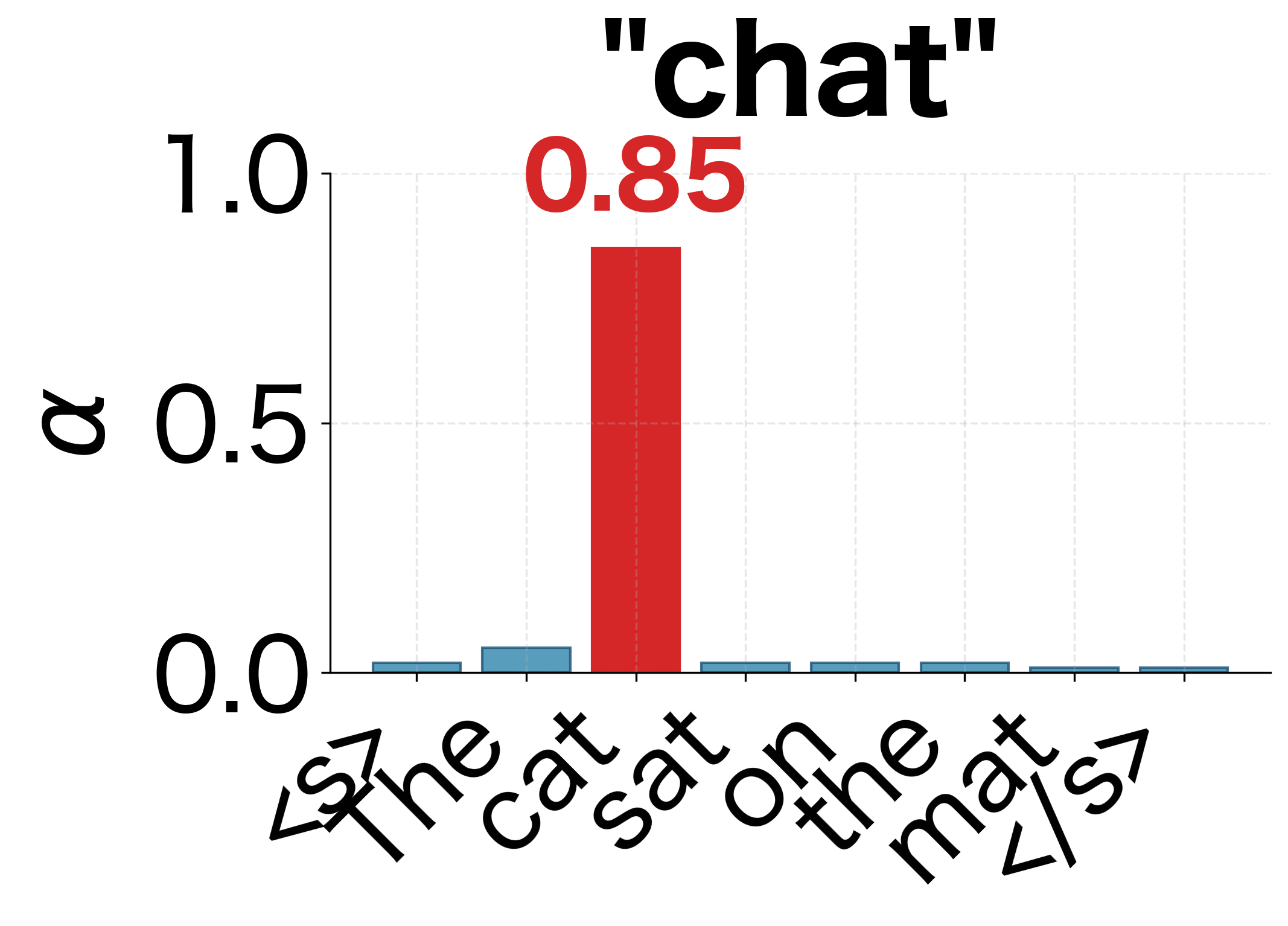
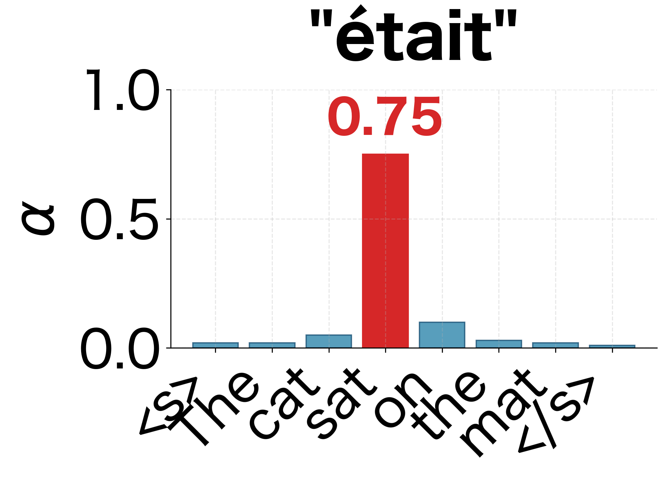
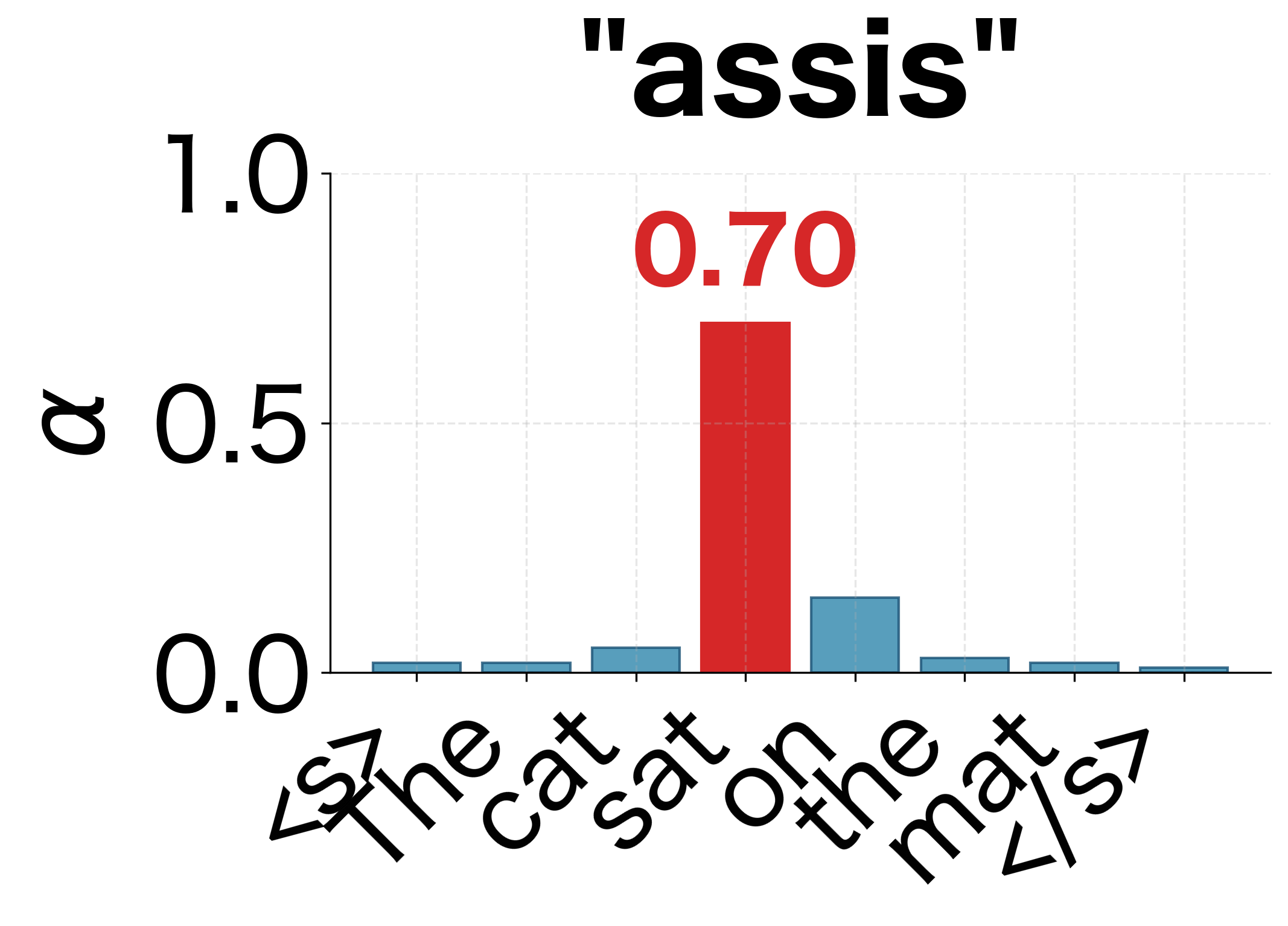
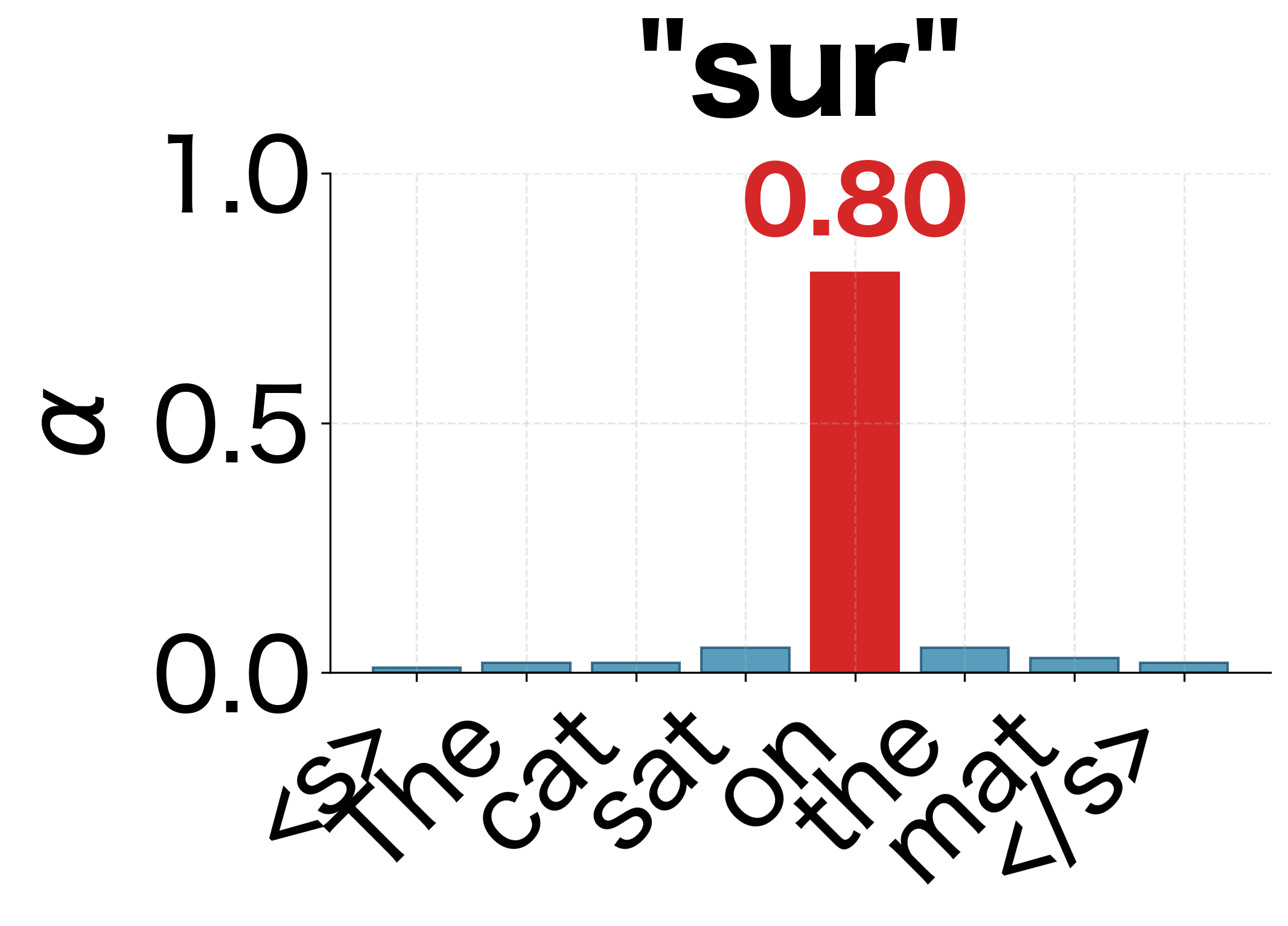
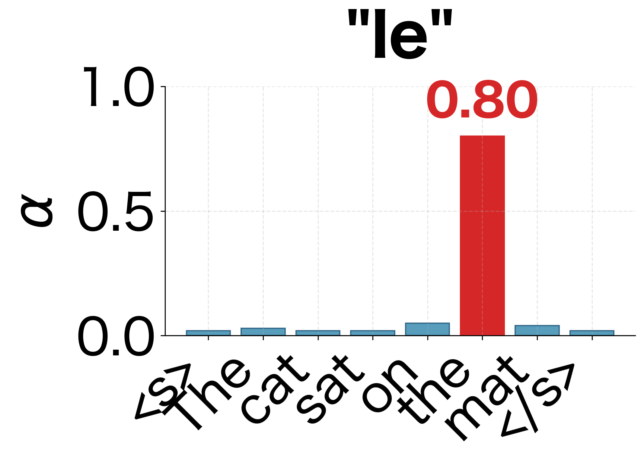
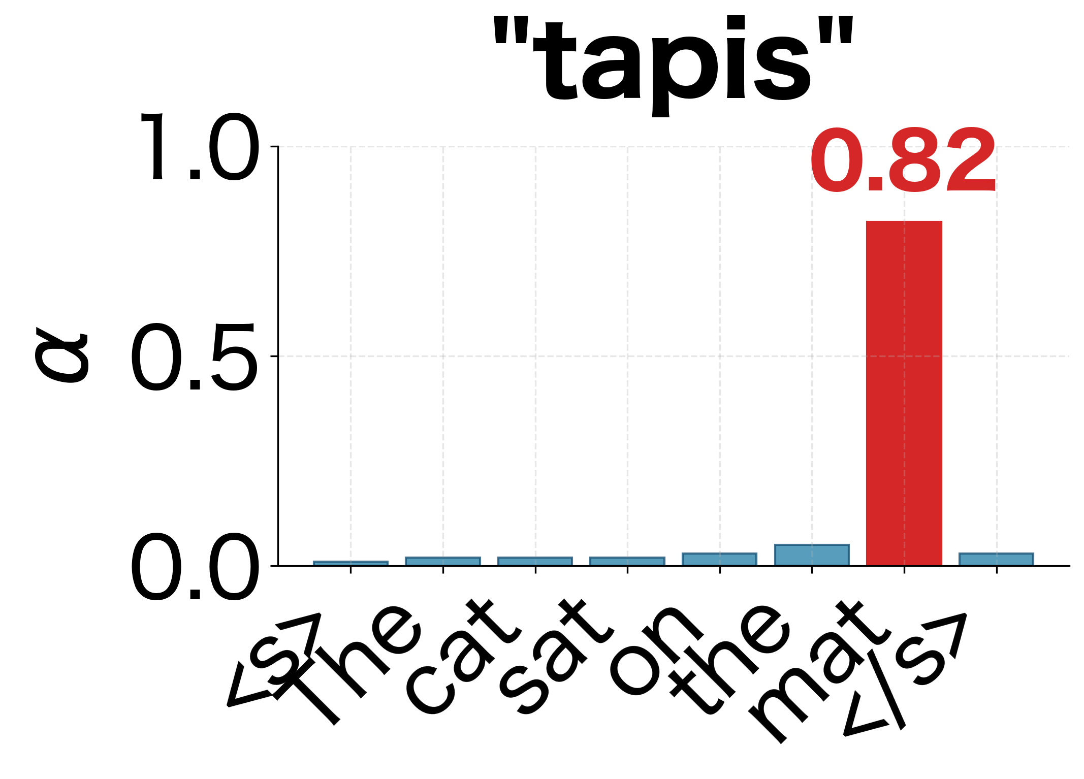
Attention mechanisms are interpretable. We can visualize the attention weights to see what the model is "looking at" when generating each output token.
The attention heatmap reveals several interesting patterns:
- Monotonic alignment: For this simple sentence, attention roughly follows the diagonal, reflecting the similar word order between English and French.
- Word-to-word correspondence: "Le" attends strongly to "The," "chat" to "cat," and "tapis" to "mat."
- Many-to-one mapping: Both "était" and "assis" attend primarily to "sat," since the single English word requires two French words.
- Soft attention: Even when one position dominates, other positions receive small but non-zero weights.
We can also visualize how the attention distribution evolves step by step during decoding. Each row in the heatmap above represents a single decoding step, but viewing them as individual distributions makes the shifting focus more apparent:
This interpretability is valuable for debugging and understanding model behavior. If a translation is wrong, we can inspect the attention weights to see if the model was looking at the right parts of the input.
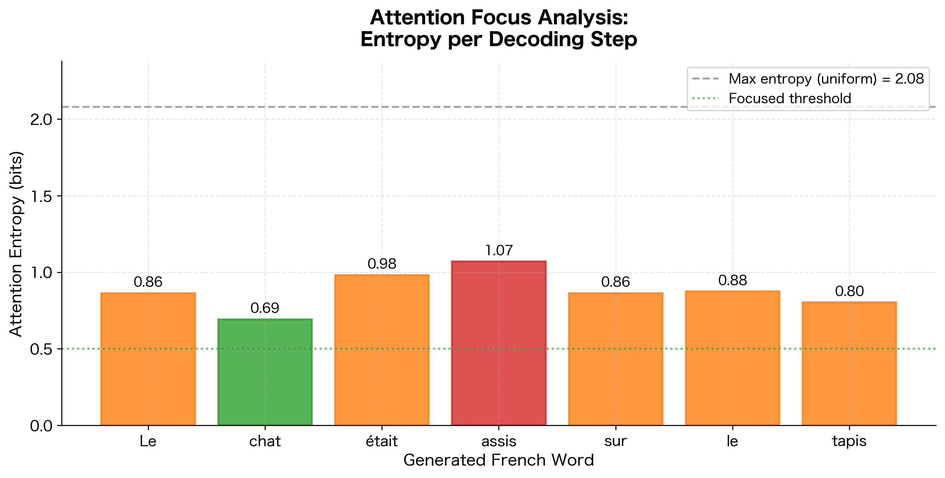
Attention Entropy: Measuring Focus
A useful metric for understanding attention behavior is entropy, which quantifies how spread out or focused the attention distribution is. Low entropy indicates concentrated attention on few positions; high entropy indicates diffuse attention across many positions.
The entropy analysis reveals that most decoding steps in this translation have relatively focused attention (entropy below 1.0), indicating clear word-to-word correspondences. Steps with higher entropy might indicate cases where the model needs to aggregate information from multiple source positions, such as translating idiomatic expressions or handling word reordering.
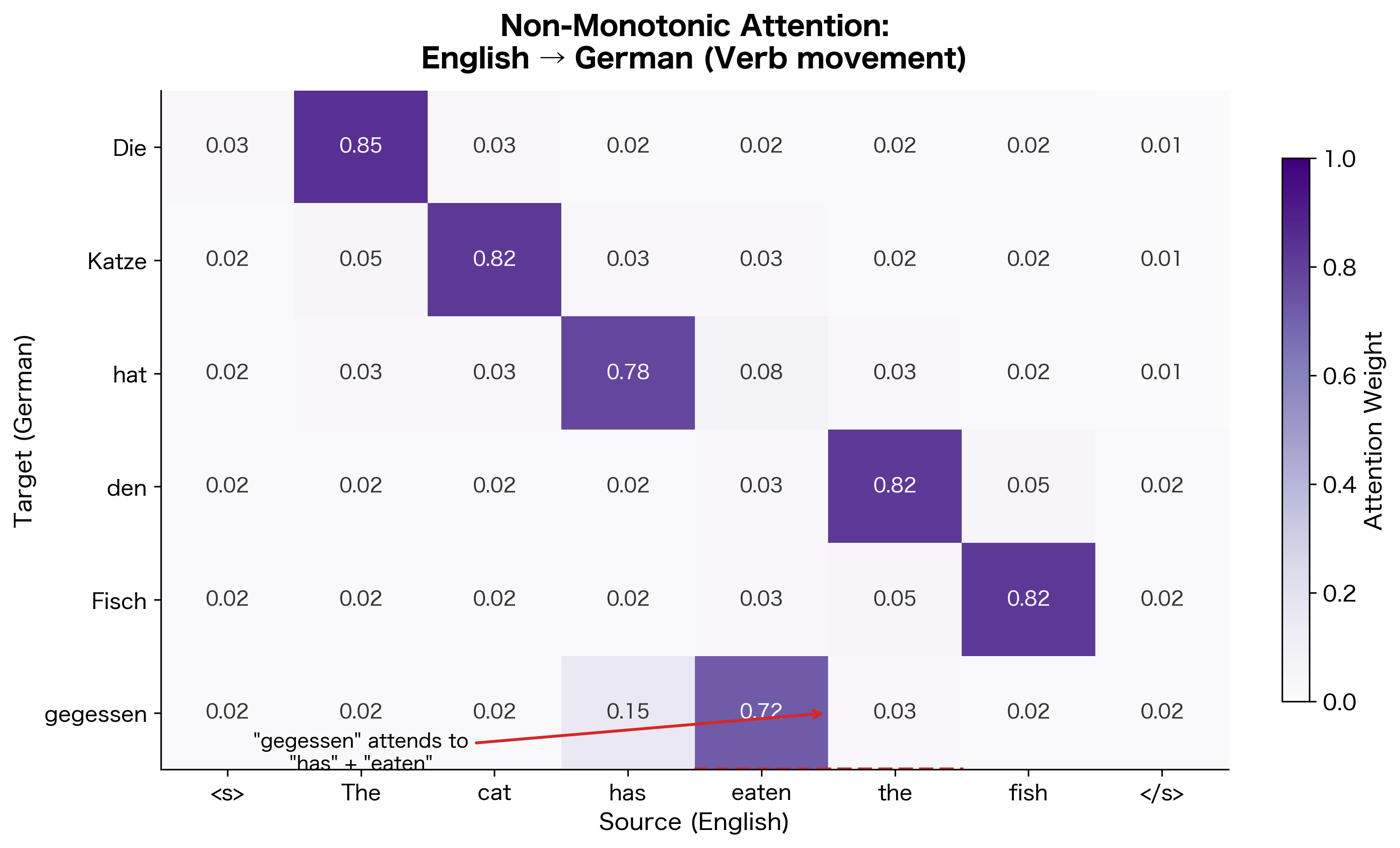
Non-Monotonic Alignment Patterns
While English-French translation often exhibits roughly monotonic alignment (words appear in similar order), attention can handle more complex patterns. Languages with different word orders, or sentences with long-distance dependencies, produce non-monotonic attention patterns.
This example demonstrates one of attention's key strengths: it can learn arbitrary alignment patterns without explicit supervision. The model discovers that German places the past participle ("gegessen") at the end of the clause, and learns to attend to the corresponding English words ("has eaten") regardless of their position.
Computational Considerations
Bahdanau attention introduces additional computation compared to a standard encoder-decoder. Let's analyze the complexity by examining each operation required at every decoder step.
For each decoder step, we must perform the following operations:
- Project the decoder state: Computing requires operations (matrix-vector multiplication)
- Project all encoder states: Computing for all requires operations
- Compute scores: The addition, tanh, and dot product with require operations
- Apply softmax: Normalizing scores requires operations
- Compute weighted sum: Computing requires operations
where:
- : source sequence length
- : target sequence length
- : decoder hidden dimension
- : encoder hidden dimension
- : alignment dimension
The dominant term is the encoder projection, which is per decoder step. Over an entire output sequence of length , the total complexity becomes . This quadratic dependence on sequence lengths () becomes significant for long sequences.
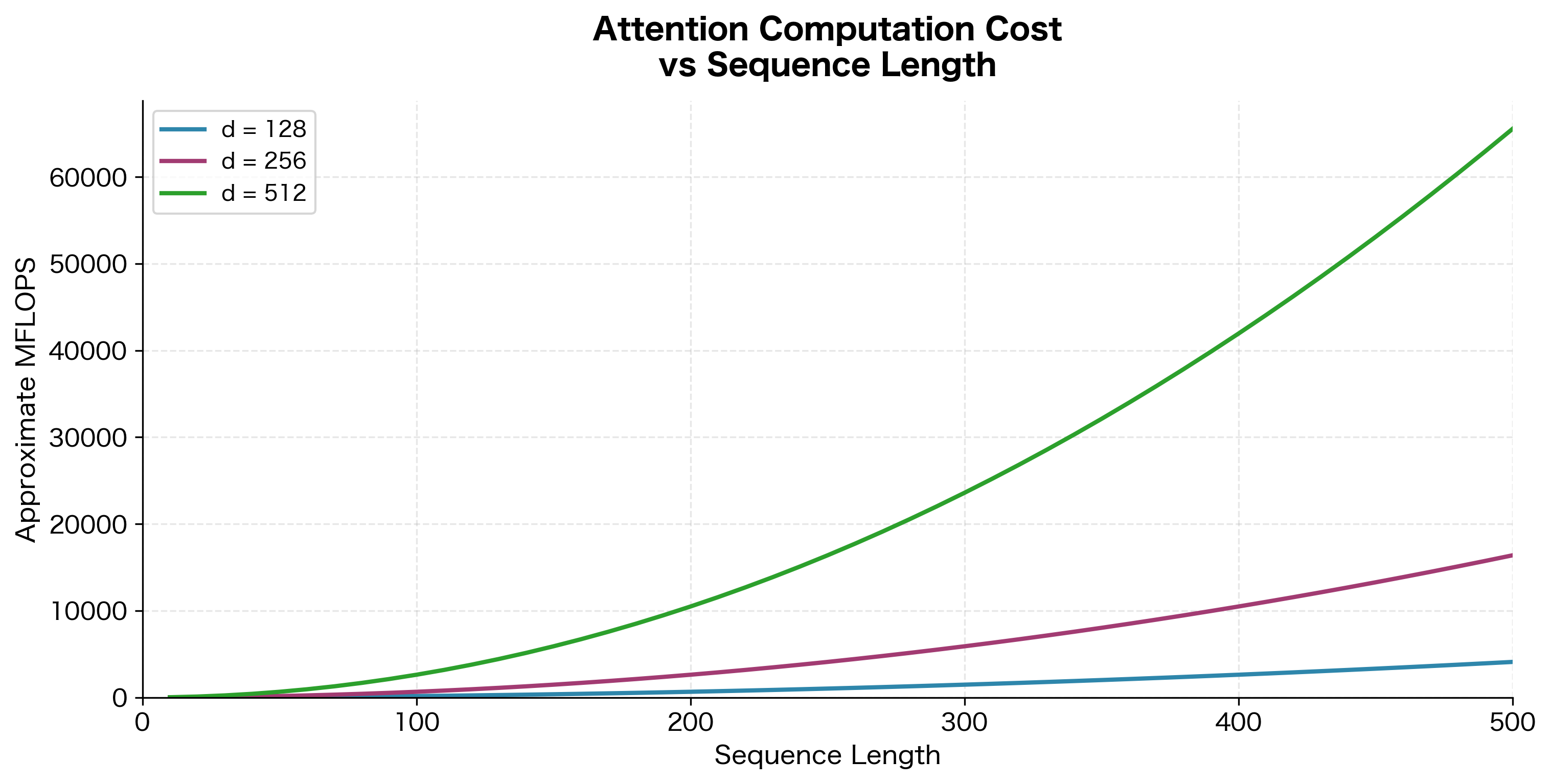
For typical machine translation tasks with sequences of 20-50 tokens, this overhead is manageable. However, for very long sequences (documents, conversations), the quadratic scaling becomes problematic. This motivated later work on efficient attention variants, which we'll explore in subsequent chapters.
A practical optimization addresses the redundant computation in step 2. Notice that the encoder projections depend only on the encoder outputs, which remain constant throughout decoding. By precomputing these projections once after encoding and caching them, we avoid repeating this computation at every decoder step:
Limitations and Impact
Bahdanau attention changed how we think about sequence-to-sequence models. However, it has several limitations that motivated subsequent research.
The most significant limitation is the sequential nature of decoding. Because attention at step depends on the decoder state , and depends on the attention at step , we cannot parallelize across decoder timesteps. Each step must wait for the previous step to complete. This sequential bottleneck limits training throughput on modern parallel hardware like GPUs, where we'd prefer to process many positions simultaneously.
Another limitation is the additive score function's computational cost. Computing requires more operations than simpler alternatives like dot-product attention. While the difference is small for individual computations, it adds up over millions of training examples. Luong attention, which we'll cover in the next chapter, addresses this with more efficient score functions.
The attention mechanism also introduces additional hyperparameters (the alignment dimension ) and learnable parameters (, , ). While these provide flexibility, they also increase the risk of overfitting on small datasets and require careful tuning.
Despite these limitations, Bahdanau attention had a major impact on the field. It showed that attention mechanisms could improve performance on sequence-to-sequence tasks, reducing the BLEU score gap between neural and phrase-based machine translation systems. It also introduced the core ideas that would evolve into the self-attention mechanism at the heart of Transformers.
The key insights that carried forward include:
- Dynamic context: Computing a fresh context vector at each decoding step, rather than using a fixed representation
- Soft alignment: Learning to align input and output positions without explicit supervision
- Interpretability: Attention weights provide insight into model behavior
- Differentiable lookup: Treating attention as a soft, differentiable lookup table
These ideas laid the groundwork for the attention-based models that would reshape NLP over the following years.
How Attention Learns: From Random to Meaningful
A natural question is: how does attention learn to produce meaningful alignments? At initialization, the attention weights are random. Through training, the model gradually discovers which source positions are relevant for each target position.
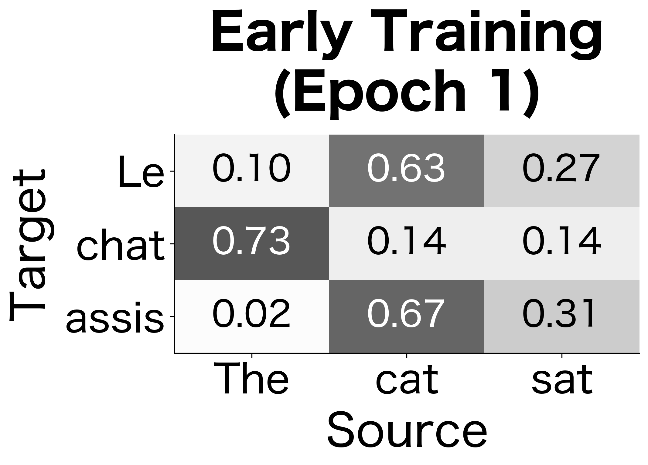
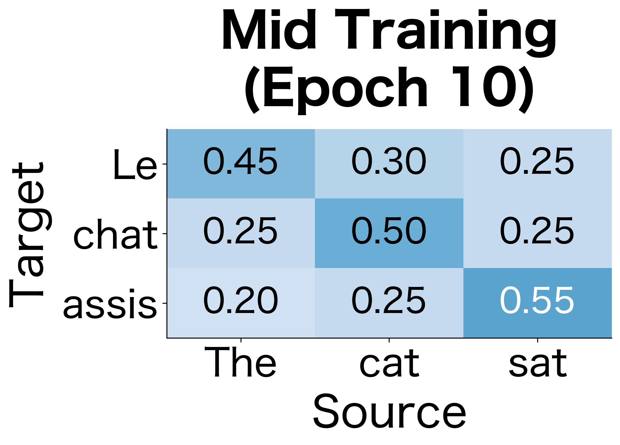
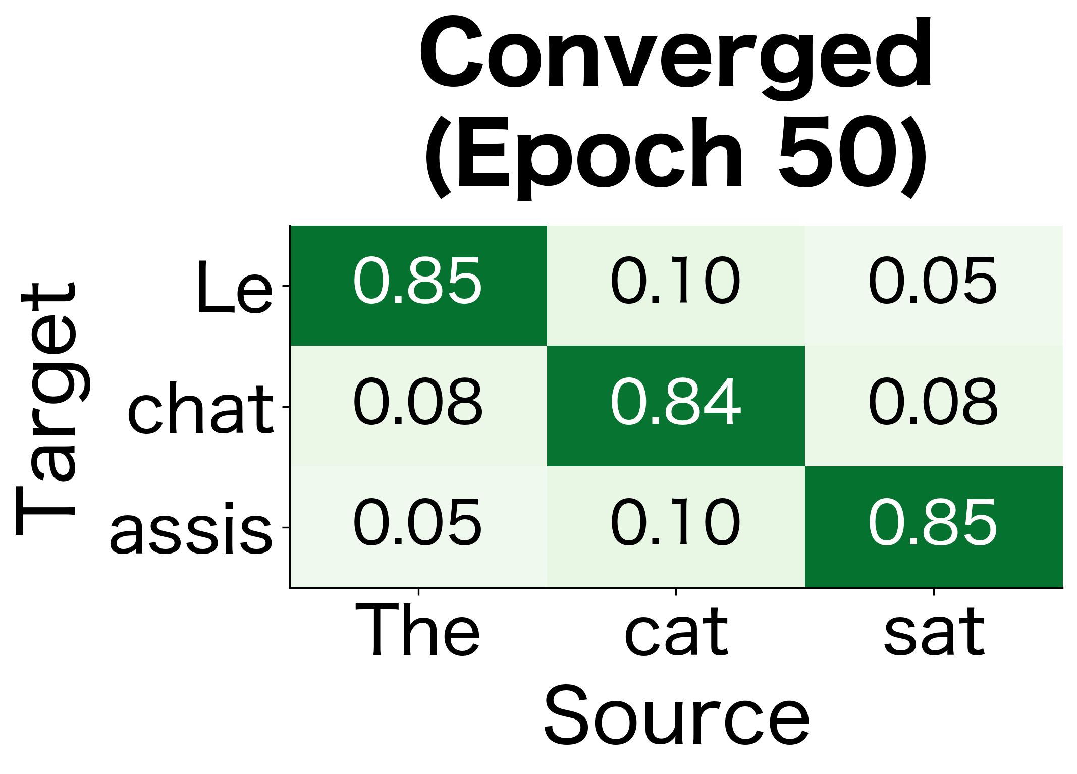
The learning progression illustrates a key property of attention: it's trained end-to-end with the translation objective. The model receives no explicit supervision about which source words correspond to which target words. Instead, it discovers these alignments because they help minimize the translation loss. This emergent alignment is one of the most interesting aspects of attention mechanisms.
Summary
Bahdanau attention solves the bottleneck problem in encoder-decoder models by allowing the decoder to dynamically focus on relevant parts of the input at each generation step. The mechanism works through a learned alignment model that scores how well each encoder position matches the current decoder state.
The key components are:
- Additive score function: computes alignment scores by projecting the decoder state and encoder states into a shared alignment space, combining them additively, and reducing to a scalar
- Softmax normalization: converts raw scores to attention weights that form a probability distribution over encoder positions
- Context vector: computes a weighted sum of encoder states, where the weights determine how much each position contributes to the context for generating output
The attention weights are interpretable, showing which input positions the model considers relevant for each output position. This interpretability, combined with strong empirical performance, made Bahdanau attention a foundational technique in neural machine translation and sequence-to-sequence modeling more broadly.
In the next chapter, we'll explore Luong attention, which offers alternative score functions with different computational trade-offs.
Key Parameters
When implementing Bahdanau attention, several parameters significantly impact model performance:
-
attention_dim(d_a): The dimension of the alignment space where encoder and decoder states are projected before comparison. Typical values range from 64 to 512. Larger values increase model capacity but also computation cost. A common heuristic is to set this equal to the encoder or decoder hidden dimension. -
encoder_dim(d_h): The dimension of encoder hidden states. For bidirectional encoders, this is typically twice the base RNN hidden size (forward + backward concatenated). Values of 256-1024 are common in practice. -
decoder_dim(d_s): The dimension of decoder hidden states. Often set equal to the encoder dimension for simplicity, though they can differ. The decoder dimension affects both the attention computation and the output projection. -
embed_dim: The dimension of word embeddings fed to the decoder. Typical values are 128-512. Smaller embeddings reduce parameters but may limit expressiveness for large vocabularies. -
vocab_size: The size of the output vocabulary. Larger vocabularies require more parameters in the output projection layer and can slow down training due to the softmax computation over all tokens.
Quiz
Ready to test your understanding? Take this quick quiz to reinforce what you've learned about Bahdanau attention and its role in neural machine translation.

Comments