Backpropagation Through Time: Training RNNs with Gradient Flow

In the previous chapter, we introduced RNN architecture: how recurrent connections create a hidden state that flows across timesteps, enabling the network to process sequences of arbitrary length. We saw the elegant parameter sharing that makes RNNs practical. But we left a critical question unanswered: how do we actually train these networks?

Standard backpropagation, which you learned in the neural network foundations, assumes a feedforward structure where information flows in one direction. RNNs break this assumption. The same weights are used at every timestep, and the hidden state at time $t$ depends on the hidden state at time $t-1$, which depends on $t-2$, and so on. This creates a temporal dependency chain that standard backpropagation cannot directly handle.

Backpropagation Through Time (BPTT) solves this problem by conceptually "unrolling" the RNN across time, transforming the recurrent network into a deep feedforward network with shared weights. Once unrolled, we can apply the chain rule just as we did for feedforward networks, but now the gradients flow backward through time as well as through layers.

This chapter derives BPTT from first principles, traces gradient flow through the unrolled computation graph, and implements the algorithm from scratch. You'll see exactly how gradients accumulate across timesteps and why this creates both computational challenges and the infamous vanishing gradient problem that we'll tackle in the next chapter.

Let's first recall how we train feedforward networks, then see why RNNs require a different approach.

In a feedforward network, each layer transforms its input exactly once. The loss depends on the final output, and backpropagation traces gradients backward through each layer. Each weight appears in exactly one place in the computation graph, so its gradient is computed once.

RNNs are fundamentally different. Consider a sequence of length $T$. At each timestep $t$, the RNN computes:

where:

• $\mathbf{h}_t \in \mathbb{R}^{d_h}$: the hidden state at timestep $t$
• $\mathbf{h}_{t-1} \in \mathbb{R}^{d_h}$: the hidden state from the previous timestep
• $\mathbf{x}_t \in \mathbb{R}^{d_x}$: the input at timestep $t$
• $\mathbf{W}_{hh} \in \mathbb{R}^{d_h \times d_h}$: the hidden-to-hidden weight matrix (recurrent weights)
• $\mathbf{W}_{xh} \in \mathbb{R}^{d_h \times d_x}$: the input-to-hidden weight matrix
• $\mathbf{b}_h \in \mathbb{R}^{d_h}$: the bias vector

The key observation is that $\mathbf{W}_{hh}$, $\mathbf{W}_{xh}$, and $\mathbf{b}_h$ are the same parameters at every timestep. This parameter sharing is what gives RNNs their power, but it also means each parameter affects the loss through multiple computational paths, one for each timestep.

The conceptual trick that makes BPTT work is unrolling: we create a copy of the RNN for each timestep, treating the recurrent network as a very deep feedforward network where each "layer" corresponds to a timestep.

Consider a sequence of length 4. The unrolled computation graph looks like this:

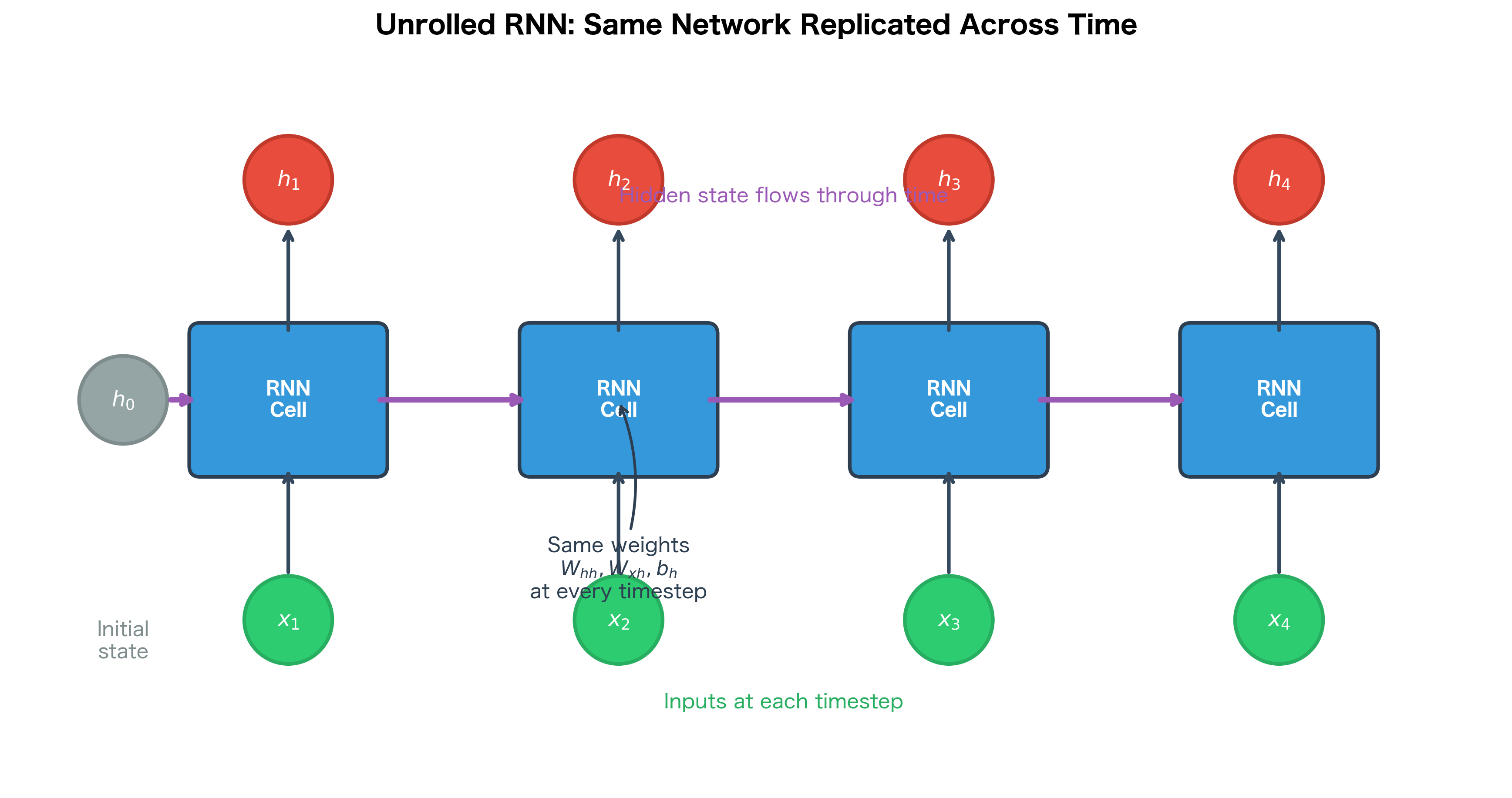
In the unrolled view, we see that:

• Each timestep has its own copy of the RNN cell, but they all share the same weights
• The hidden state $\mathbf{h}_t$ flows horizontally, carrying information from past to future
• Inputs $\mathbf{x}_t$ enter from below at each timestep
• The network is now a deep feedforward network with $T$ "layers"

This unrolling is purely conceptual. We don't actually create $T$ copies of the weights in memory. But thinking about the RNN this way allows us to apply the chain rule systematically.

With the unrolled view in mind, we can now derive the BPTT algorithm systematically. The key challenge is this: how do we compute the gradient of the loss with respect to weights that are used repeatedly across time? The answer comes from carefully applying the chain rule while tracking how each weight influences the loss through multiple paths.

We'll build up the derivation in three stages, starting with the simplest case and progressively tackling more complex dependencies:

1. Output weights (straightforward: no temporal dependencies)
2. Hidden state gradients (the recursive heart of BPTT)
3. Recurrent weights (combining recursion with gradient accumulation)

Throughout, we'll consider a sequence-to-sequence task where we compute a loss at each timestep and sum them. The total loss over the entire sequence is:

where:

• $\mathcal{L}$: the total loss over all timesteps, which we want to minimize
• $T$: the sequence length (total number of timesteps)
• $\mathcal{L}_t$: the loss at timestep $t$, typically computed from the hidden state $\mathbf{h}_t$ through an output layer (e.g., cross-entropy for classification)

We begin with the simplest case: the output weights $\mathbf{W}_{hy}$ that transform hidden states into predictions. This serves as a warm-up because these weights don't create temporal dependencies. Each use of $\mathbf{W}_{hy}$ at timestep $t$ affects only the loss $\mathcal{L}_t$ at that timestep, not any future losses.

If we have an output layer that produces predictions from the hidden state:

where:

• $\mathbf{y}_t \in \mathbb{R}^{d_y}$: the output (logits) at timestep $t$
• $\mathbf{W}_{hy} \in \mathbb{R}^{d_y \times d_h}$: the hidden-to-output weight matrix
• $\mathbf{h}_t \in \mathbb{R}^{d_h}$: the hidden state at timestep $t$
• $\mathbf{b}_y \in \mathbb{R}^{d_y}$: the output bias vector

The gradient with respect to $\mathbf{W}_{hy}$ is straightforward because $\mathbf{W}_{hy}$ only affects the loss through the outputs at each timestep. Applying the chain rule:

where:

• $\frac{\partial \mathcal{L}}{\partial \mathbf{W}_{hy}}$: the total gradient of the loss with respect to the output weights
• $\frac{\partial \mathcal{L}_t}{\partial \mathbf{y}_t}$: the gradient of the loss at timestep $t$ with respect to the output, which depends on your loss function (e.g., softmax cross-entropy)
• $\mathbf{h}_t^\top$: the transpose of the hidden state, needed for the outer product that produces a matrix gradient

This is just standard backpropagation applied independently at each timestep, then summed. The output weights are straightforward because they don't create temporal dependencies: changing $\mathbf{W}_{hy}$ at timestep 3 doesn't affect the hidden state at timestep 4.

Now we tackle the heart of BPTT: computing gradients for the hidden states. This is where temporal dependencies make things interesting, and where the "through time" in BPTT becomes essential.

Consider the hidden state $\mathbf{h}_t$ at some timestep $t$. In a feedforward network, each activation affects the loss through exactly one path. But in an RNN, $\mathbf{h}_t$ influences the loss through two distinct channels:

1. Direct effect: $\mathbf{h}_t$ produces output $\mathbf{y}_t$, which contributes to loss $\mathcal{L}_t$
2. Indirect effect: $\mathbf{h}_t$ flows into $\mathbf{h}_{t+1}$, which affects $\mathcal{L}_{t+1}$, and then into $\mathbf{h}_{t+2}$, affecting $\mathcal{L}_{t+2}$, and so on through all future timesteps

This dual influence is the fundamental difference from feedforward networks. The total gradient must account for both channels, which leads us to a recursive formulation.

For the final timestep $T$, the gradient is simple because there are no future timesteps to consider:

For earlier timesteps, we must account for both the direct contribution to $\mathcal{L}_t$ and the indirect contribution through future hidden states. The multivariate chain rule gives us:

where:

• $\frac{\partial \mathcal{L}}{\partial \mathbf{h}_t}$: the total gradient of the loss with respect to hidden state $\mathbf{h}_t$, accounting for all paths to the loss
• $\frac{\partial \mathcal{L}_t}{\partial \mathbf{h}_t}$: the direct gradient from the loss at timestep $t$ (through the output layer)
• $\frac{\partial \mathcal{L}}{\partial \mathbf{h}_{t+1}}$: the total gradient at the next timestep (already computed when working backward)
• $\frac{\partial \mathbf{h}_{t+1}}{\partial \mathbf{h}_t}$: how much $\mathbf{h}_{t+1}$ changes when we perturb $\mathbf{h}_t$ (the Jacobian of the RNN transition)

This recursive formula is the heart of BPTT. To make the recursion explicit, let's define $\boldsymbol{\delta}_t = \frac{\partial \mathcal{L}}{\partial \mathbf{h}_t}$ as the "error signal" at timestep $t$. This gives us:

The term $\frac{\partial \mathbf{h}_{t+1}}{\partial \mathbf{h}_t}$ is the Jacobian of the hidden state transition. To derive it, recall that $\mathbf{h}_{t+1} = \tanh(\mathbf{W}_{hh}\mathbf{h}_t + \mathbf{W}_{xh}\mathbf{x}_{t+1} + \mathbf{b}_h)$. Applying the chain rule:

where:

• $\text{diag}(1 - \mathbf{h}_{t+1}^2)$: a diagonal matrix of size $d_h \times d_h$, where the $i$-th diagonal entry is $(1 - h_{t+1,i}^2)$, the derivative of tanh at the $i$-th hidden unit
• $\mathbf{W}_{hh}$: the recurrent weight matrix, which determines how the previous hidden state influences the current one

The tanh derivative $(1 - h^2)$ ranges from 0 (when $h = \pm 1$, the saturation regions) to 1 (when $h = 0$). This bounded derivative will become critically important when we discuss vanishing gradients: if the hidden units saturate (approach $\pm 1$), the gradient signal gets attenuated at each timestep.

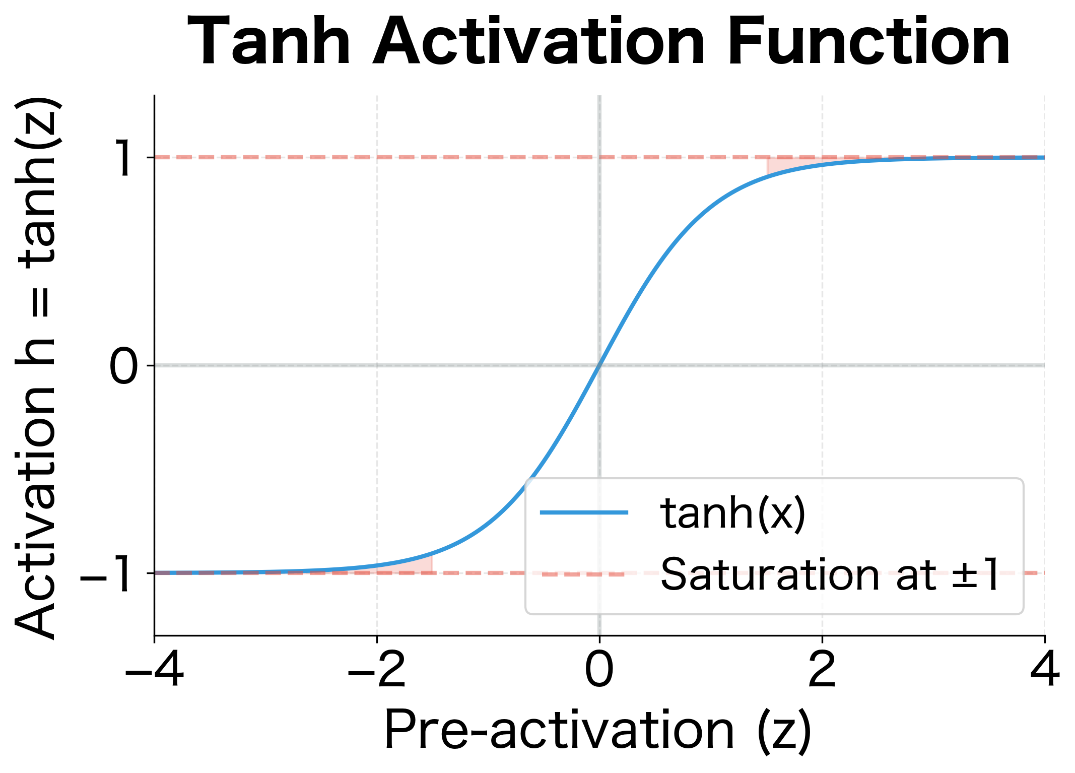
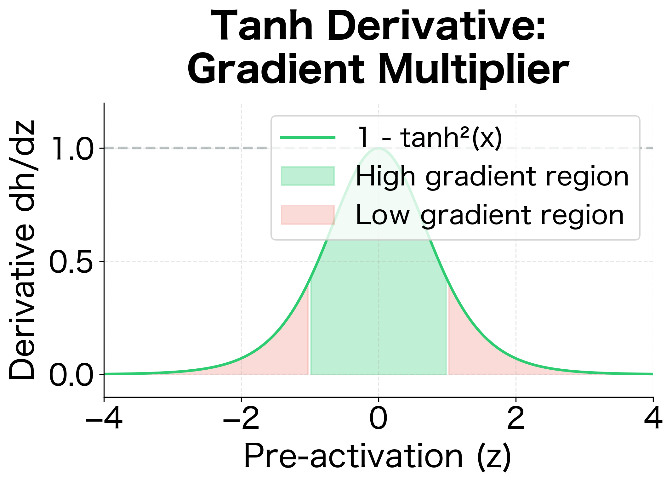
The plot reveals why tanh can cause gradient problems. In the green region (|z| < 1), the derivative is close to 1, allowing gradients to flow relatively unimpeded. But in the red saturation regions (|z| > 1), the derivative drops rapidly toward zero. If hidden units frequently saturate, each timestep multiplies the gradient by a small number, causing exponential decay.

With the hidden state gradients in hand, we can finally tackle the recurrent weights $\mathbf{W}_{hh}$. This is where gradient accumulation becomes essential.

The challenge is that $\mathbf{W}_{hh}$ appears at every timestep in the unrolled computation graph. When we change $\mathbf{W}_{hh}$, we change the computation at timestep 1, timestep 2, timestep 3, and so on. Each of these changes affects the loss. The total gradient must sum all these contributions:

More formally, since $\mathbf{W}_{hh}$ is used at every timestep, its gradient is the sum of contributions from all timesteps:

where:

• $\frac{\partial \mathcal{L}}{\partial \mathbf{W}_{hh}}$: the total gradient of the loss with respect to the recurrent weights
• $\frac{\partial \mathcal{L}}{\partial \mathbf{h}_t} = \boldsymbol{\delta}_t$: the error signal at timestep $t$ (computed in the backward pass)
• $\frac{\partial \mathbf{h}_t}{\partial \mathbf{W}_{hh}}$: how the hidden state at timestep $t$ changes with respect to the weights (the local gradient)

At each timestep $t$, the local gradient comes from differentiating $\mathbf{h}_t = \tanh(\mathbf{W}_{hh}\mathbf{h}_{t-1} + \ldots)$ with respect to $\mathbf{W}_{hh}$:

where $\mathbf{h}_{t-1}^\top$ appears because the gradient of a matrix-vector product $\mathbf{W}\mathbf{v}$ with respect to $\mathbf{W}$ involves the vector $\mathbf{v}$.

Combining the error signal with the local gradient at each timestep:

where:

• $\boldsymbol{\delta}_t \odot (1 - \mathbf{h}_t^2)$: the error signal multiplied element-wise by the tanh derivative, giving the gradient at the pre-activation
• $\mathbf{h}_{t-1}^\top$: the hidden state from the previous timestep, transposed for the outer product
• $\odot$: element-wise (Hadamard) multiplication

The sum over all timesteps reflects the fact that the same weight matrix $\mathbf{W}_{hh}$ is used at every step. Each use contributes to the total gradient.

To understand BPTT intuitively, let's visualize how gradients flow backward through the unrolled network.

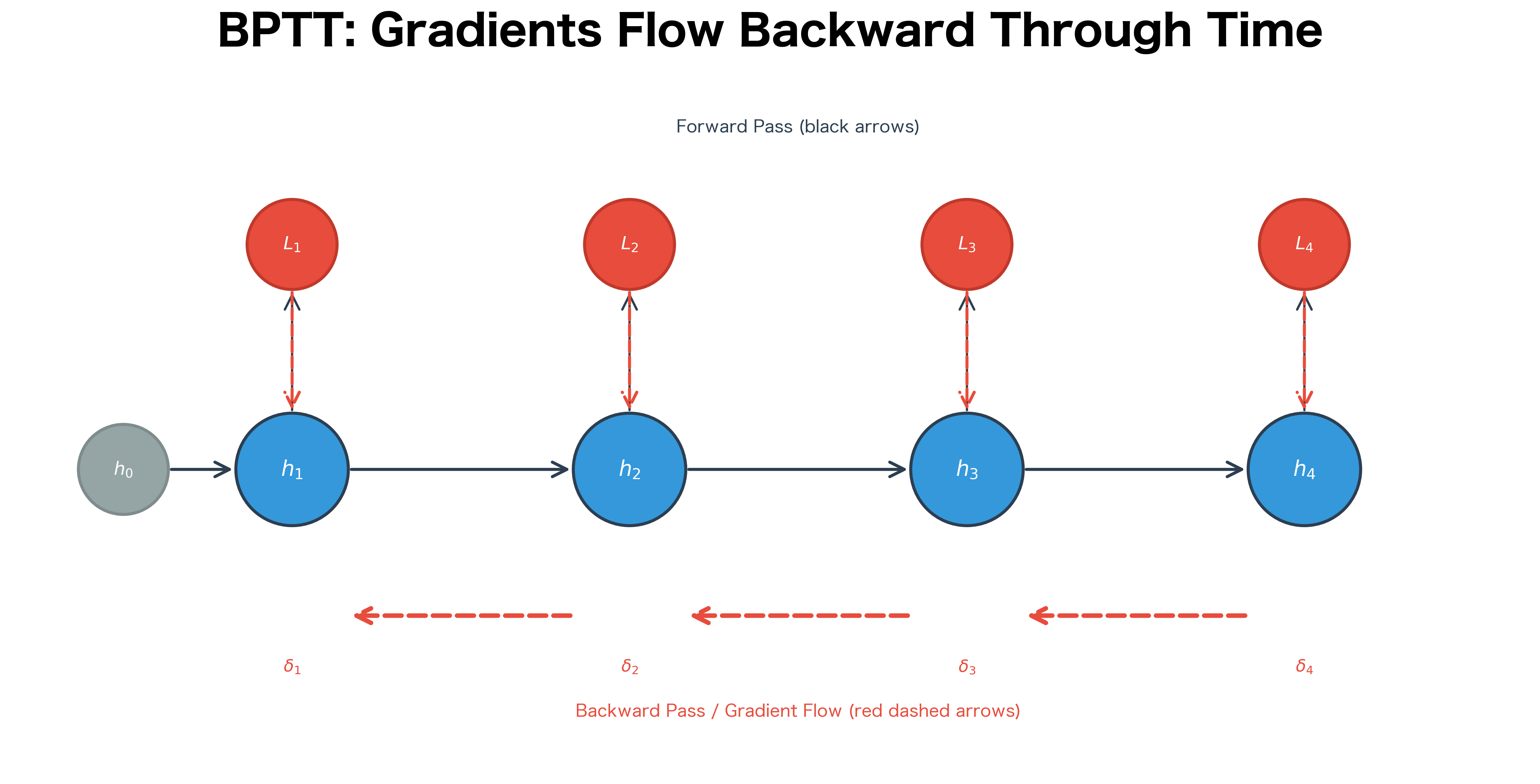
The diagram reveals a crucial insight: the gradient at early timesteps accumulates contributions from all future losses. The gradient $\boldsymbol{\delta}_1$ at the first hidden state includes:

• The direct gradient from $\mathcal{L}_1$
• The gradient from $\mathcal{L}_2$ flowing back through $\mathbf{h}_2$
• The gradient from $\mathcal{L}_3$ flowing back through $\mathbf{h}_3$ and $\mathbf{h}_2$
• The gradient from $\mathcal{L}_4$ flowing back through $\mathbf{h}_4$, $\mathbf{h}_3$, and $\mathbf{h}_2$

This accumulation is what allows RNNs to learn long-range dependencies, but it's also the source of the vanishing gradient problem we'll explore in the next chapter.

The formulas above can feel abstract until you trace through them with concrete numbers. Let's work through BPTT step by step on a tiny example, computing every intermediate value by hand. This will solidify your understanding of how gradients flow backward through time and accumulate across timesteps.

We'll use a sequence of length 3 with scalar hidden states (dimension 1) to keep the arithmetic tractable. In practice, hidden states are vectors with hundreds or thousands of dimensions, but the same principles apply.

Setup:

• Sequence length: $T = 3$
• Hidden dimension: $d_h = 1$ (scalar for simplicity)
• Input dimension: $d_x = 1$
• Inputs: $x_1 = 0.5$, $x_2 = -0.3$, $x_3 = 0.8$
• Initial hidden state: $h_0 = 0$
• Weights: $W_{hh} = 0.6$, $W_{xh} = 0.4$, $b_h = 0.1$
• Target outputs: $y_1^* = 0.3$, $y_2^* = -0.1$, $y_3^* = 0.5$
• Loss: Mean squared error at each timestep

Forward Pass:

Backward Pass:

Now we compute gradients flowing backward from $t=3$ to $t=1$:

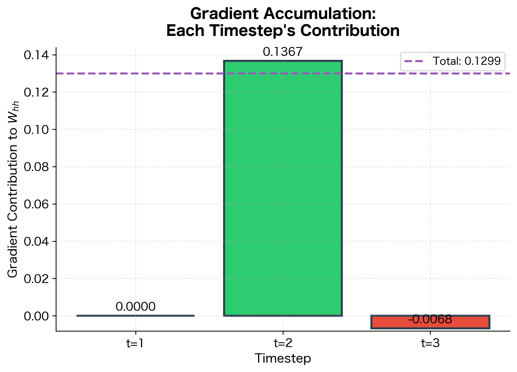
This worked example illustrates the two key aspects of BPTT:

1. Recursive gradient computation: Notice how $\delta_1$ at the first timestep includes contributions from all three losses. The gradient from $\mathcal{L}_3$ flows backward through $\mathbf{h}_3$ and $\mathbf{h}_2$ before reaching $\mathbf{h}_1$, getting multiplied by the tanh derivative and $W_{hh}$ at each step. This is the "through time" in Backpropagation Through Time.

2. Gradient accumulation for shared weights: The gradient for $W_{hh}$ is the sum of contributions from all timesteps. At timestep 1, the contribution is zero because $h_0 = 0$, but timesteps 2 and 3 both contribute. In a longer sequence, this sum would have many more terms, all computed in a single backward pass.

The small numbers in this example hint at a deeper issue: the gradient contributions shrink as we go further back in time. The tanh derivative (around 0.78-0.92 in our example) multiplied by $W_{hh} = 0.6$ gives a factor less than 1 at each step. Over many timesteps, this shrinking compounds exponentially, leading to the vanishing gradient problem we'll explore in the next chapter.

Let's visualize how gradient magnitude decays as it flows backward through time:

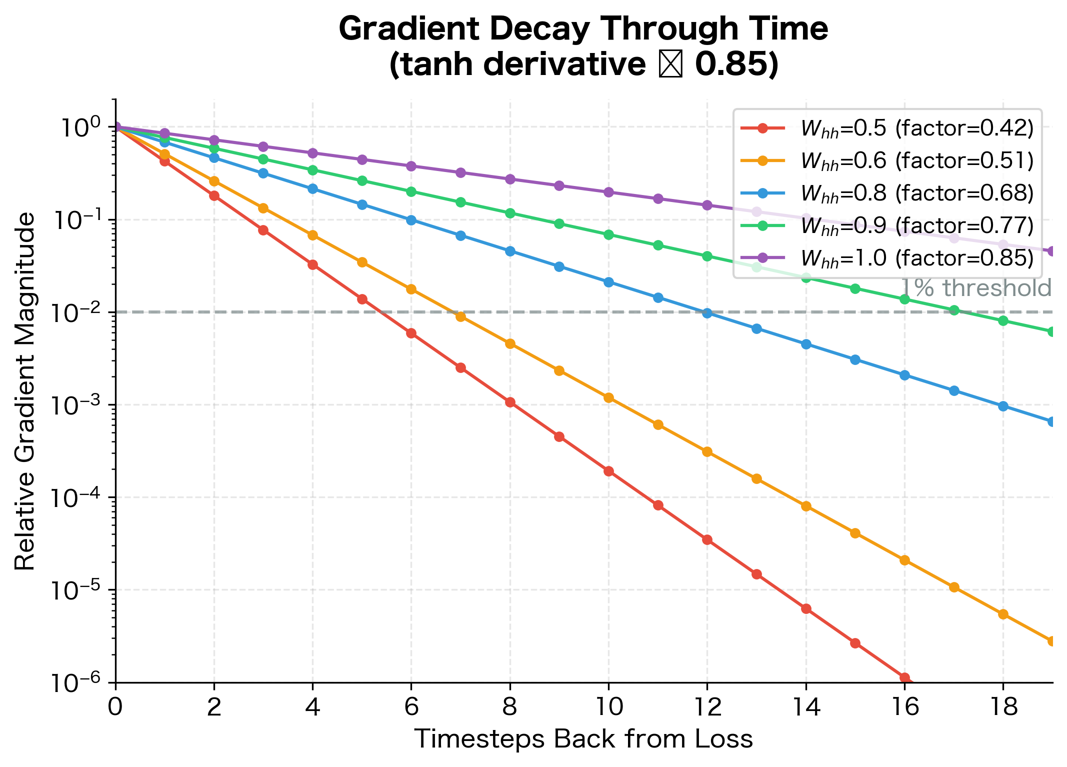
The logarithmic scale reveals the exponential nature of gradient decay. With $W_{hh} = 0.6$ (our worked example), gradients fall below 1% of their original magnitude after just 8 timesteps. Even with $W_{hh} = 0.9$, gradients still decay significantly over 20 steps. Only when the effective decay factor approaches 1.0 do gradients maintain their magnitude, but this requires careful initialization and is difficult to maintain during training.

Having derived BPTT mathematically and traced through a worked example, we're ready to implement the algorithm in code. This implementation will handle the general case: vector-valued hidden states, multiple weight matrices, and cross-entropy loss for classification.

We'll build a simple character-level language model, a classic application of RNNs that predicts the next character given the previous characters. This task is simple enough to train quickly but complex enough to demonstrate all aspects of BPTT.

The forward pass computes hidden states and outputs while storing everything needed for backpropagation. The key insight is that we must save all intermediate values: the hidden states at every timestep (for computing weight gradients) and the pre-activation values (for computing tanh derivatives).

The forward pass stores three critical pieces of information:

• inputs: The input vectors at each timestep
• hidden_states: All hidden states including $h_0$, needed for computing weight gradients
• pre_activations: The values before tanh, needed for computing tanh derivatives

The backward pass is where BPTT comes to life. We iterate through timesteps in reverse order, computing the error signal $\boldsymbol{\delta}_t$ at each step and accumulating gradients for all weight matrices. The code directly implements the formulas we derived earlier:

The backward pass implements the BPTT algorithm:

1. Compute output gradients: For each timestep, compute the gradient of the cross-entropy loss with respect to the output logits.

2. Backward through time: Starting from the last timestep, propagate gradients backward. At each step:

   • Add the gradient from the output layer and the gradient from future timesteps
   • Backpropagate through the tanh activation
   • Accumulate gradients for all weight matrices
   • Pass the gradient to the previous timestep through $\mathbf{W}_{hh}$

3. Gradient accumulation: Each weight matrix accumulates contributions from all timesteps.

Let's verify our implementation by comparing analytical gradients to numerical approximations:

The analytical and numerical gradients match to within $10^{-7}$ relative error, well within floating-point precision. This level of agreement confirms our BPTT implementation is mathematically correct. Gradient checking is an essential debugging technique: if the relative error exceeds $10^{-5}$, there's likely a bug in the backward pass.

Let's train our RNN on a simple character prediction task:

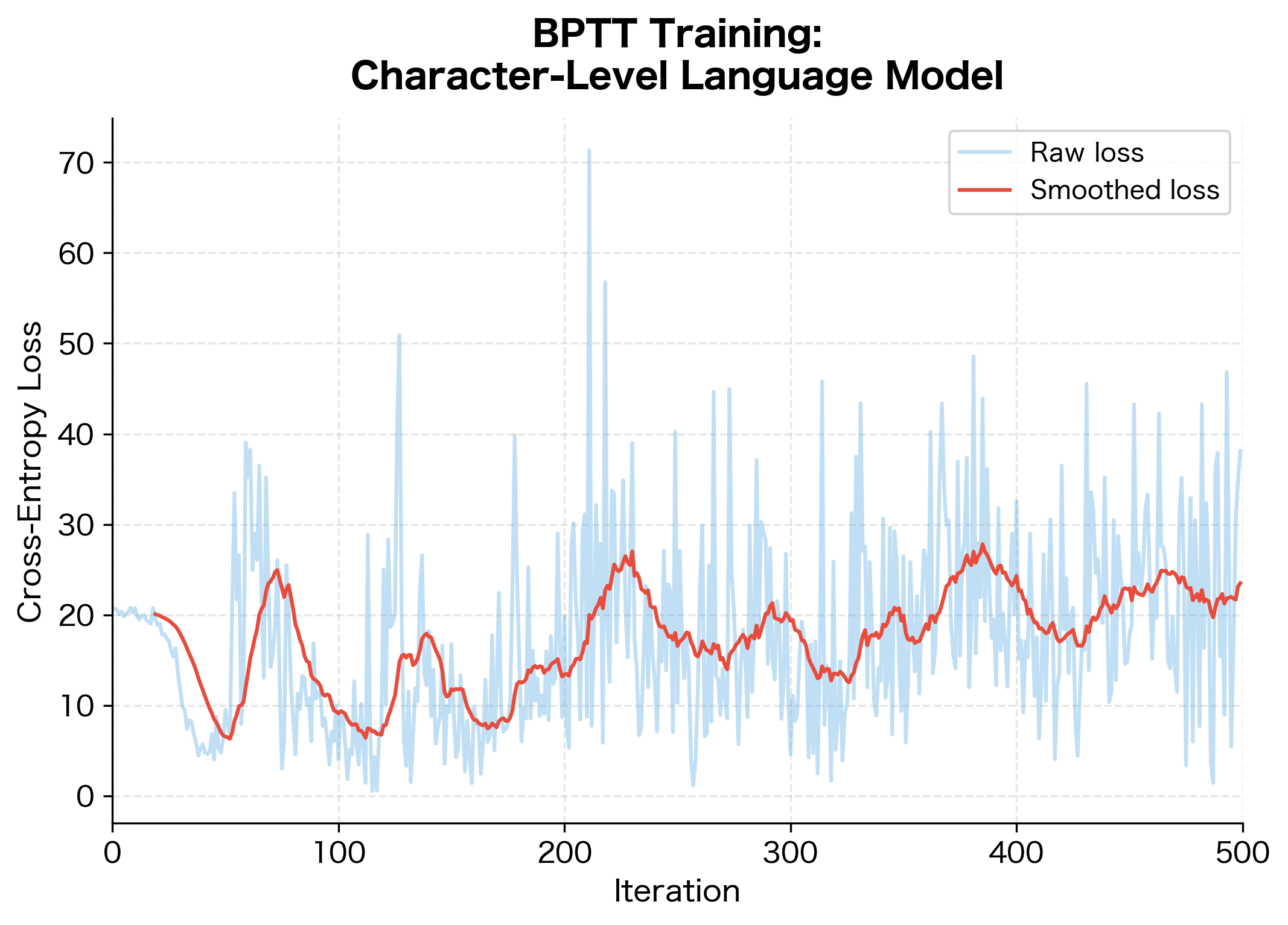
The loss decreases steadily, showing that BPTT successfully trains the RNN. Let's sample from the trained model:

The generated text shows the RNN has learned the basic structure of the training data. While not perfect (the simple model and limited training produce some errors), the output demonstrates that BPTT successfully trained the network to capture character-level patterns. The model learned common bigrams like "he", "ll", "wo", and "ld" from the repeating "hello world" sequence.

Full BPTT requires storing all hidden states for the entire sequence, which becomes prohibitive for long sequences. For a sequence of length $T$ with hidden dimension $d_h$, we need $O(T \cdot d_h)$ memory just for hidden states.

Truncated BPTT addresses this by limiting how far back gradients flow. Instead of backpropagating through the entire sequence, we:

1. Divide the sequence into chunks of length $k$
2. Run forward through the entire sequence, but only backpropagate through the last $k$ timesteps
3. Carry the hidden state forward between chunks, but not the gradients

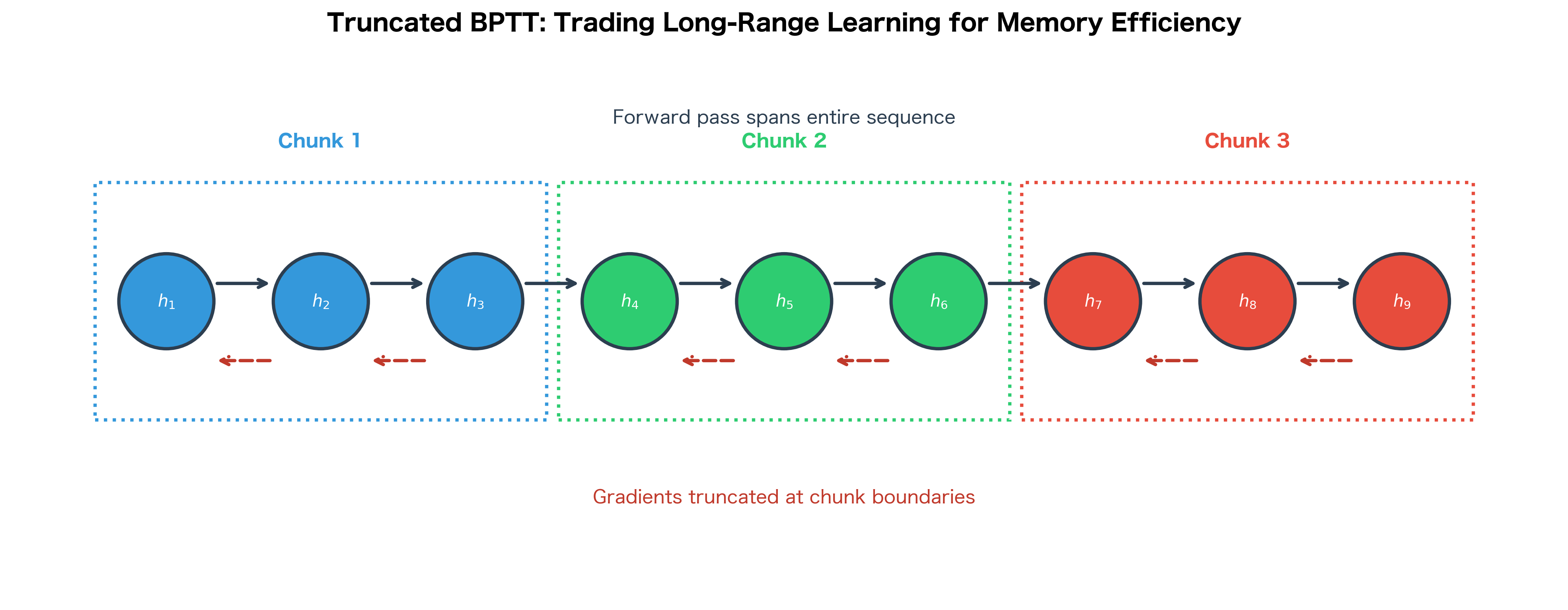
The trade-off is clear: truncated BPTT uses less memory but cannot learn dependencies longer than $k$ timesteps. In practice, $k$ is often set to 20-50 timesteps, which works well for many tasks but fundamentally limits what the RNN can learn.

Understanding BPTT's memory requirements is crucial for practical deep learning. Let's analyze what we need to store during training.

Forward Pass Storage:

• Hidden states: $T \times d_h$ values (one hidden state vector per timestep)
• Pre-activation values: $T \times d_h$ values (needed to compute tanh derivatives during backprop)
• Inputs: $T \times d_x$ values (already stored as part of the input data)

Backward Pass Computation:

• Gradient for each weight matrix: same size as the weight (e.g., $d_h \times d_h$ for $\mathbf{W}_{hh}$)
• Temporary gradient signals: $d_h$ values for $\boldsymbol{\delta}_t$ (reused at each timestep)

The dominant cost is storing hidden states: $O(T \cdot d_h)$ memory. For a sequence of length 1000 with hidden dimension 512, this is about 2 million floating-point numbers, or 8 MB in float32. With batch processing (multiple sequences simultaneously), multiply by the batch size.

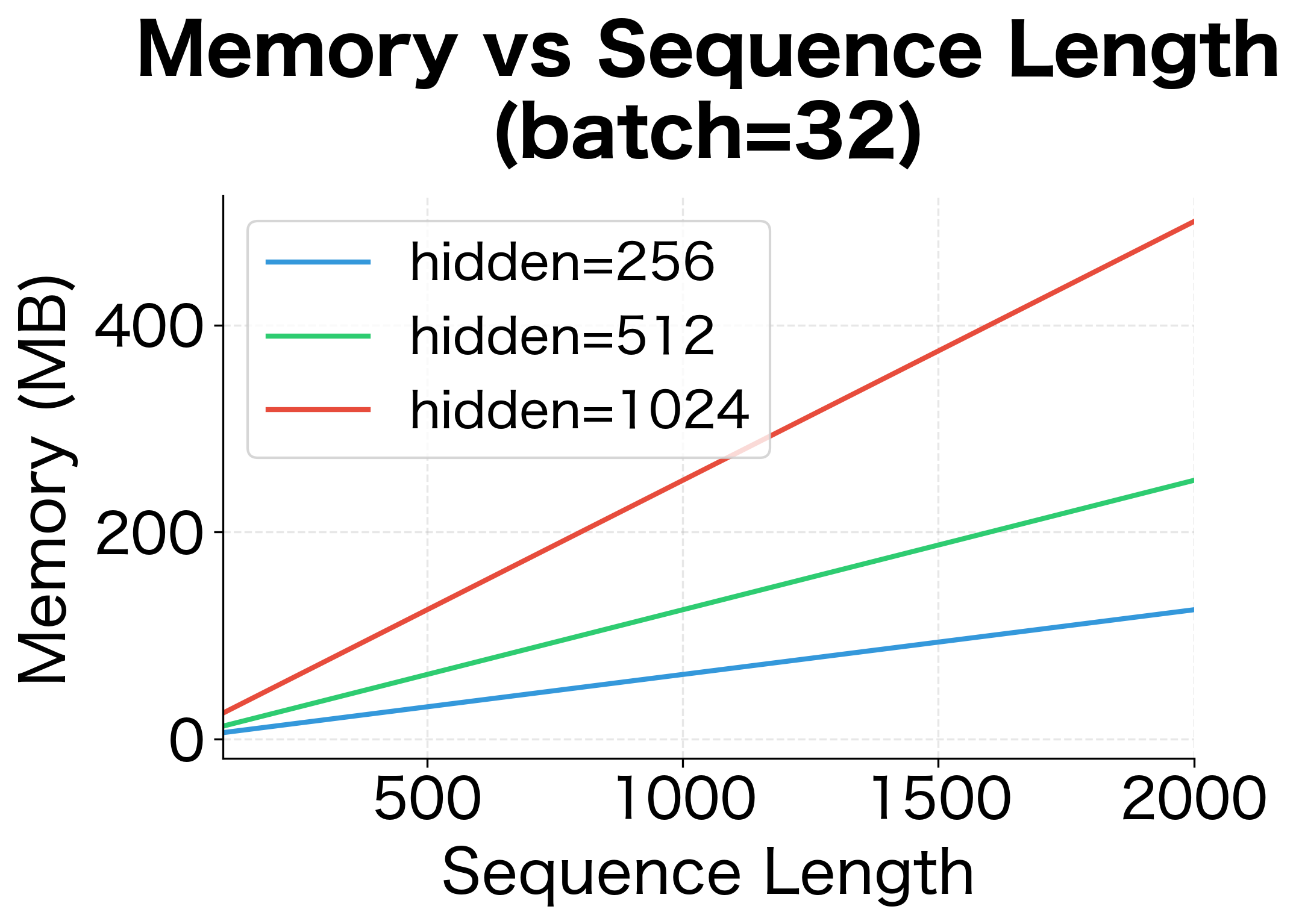
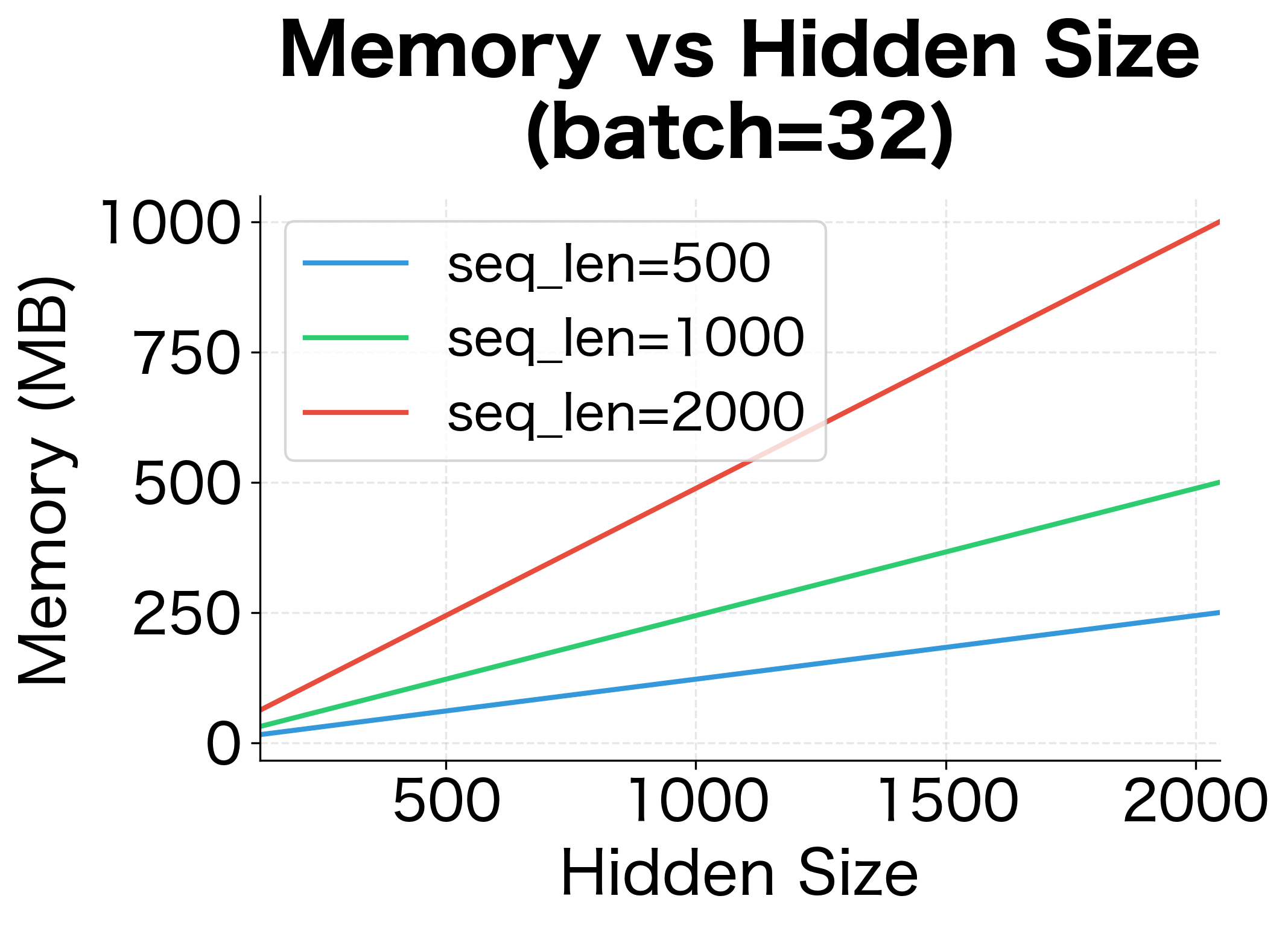
The table and plots show how memory requirements scale dramatically with sequence length, hidden size, and batch size. A modest configuration (1000 timesteps, 1024 hidden units, batch size 64) already requires over 500 MB just for activation storage, not including model parameters or optimizer state. For very long sequences, memory becomes the bottleneck. This is one motivation for truncated BPTT and later architectural innovations like transformers that can process sequences in parallel.

BPTT is a foundational algorithm that made training recurrent neural networks practical, but it comes with significant challenges that shaped the evolution of sequence modeling.

The most critical limitation of BPTT is the vanishing gradient problem. When gradients flow backward through many timesteps, they pass through repeated multiplications by $\mathbf{W}_{hh}$ and the tanh derivative $(1 - h^2)$. If these multiplications consistently shrink the gradient (eigenvalues less than 1), the gradient signal decays exponentially.

To see this mathematically, consider how the gradient at $\mathbf{h}_1$ depends on the loss at timestep $T$. Unrolling the recursive formula, we get a product of Jacobians:

where:

• $\frac{\partial \mathcal{L}_T}{\partial \mathbf{h}_1}$: how much the loss at the final timestep changes when we perturb the first hidden state
• $\frac{\partial \mathcal{L}_T}{\partial \mathbf{h}_T}$: the direct gradient at the final timestep
• $\prod_{t=2}^{T} \frac{\partial \mathbf{h}_t}{\partial \mathbf{h}_{t-1}}$: the product of $T-1$ Jacobian matrices, each of the form $\text{diag}(1 - \mathbf{h}_t^2) \cdot \mathbf{W}_{hh}$

Each Jacobian has magnitude bounded by the product of the largest tanh derivative (at most 1) and the spectral norm of $\mathbf{W}_{hh}$. If this product is less than 1, the gradient shrinks at each step. After $T$ steps, the gradient is multiplied by a factor that decays exponentially with sequence length.

For long sequences, this product approaches zero, meaning early timesteps receive essentially no learning signal from late losses. The network cannot learn long-range dependencies because the gradient information is lost before it reaches the relevant parameters.

This isn't just a theoretical concern. In practice, vanilla RNNs trained with BPTT struggle with dependencies beyond 10-20 timesteps. A language model might fail to connect a pronoun with its antecedent if they're separated by many words. A time series model might miss patterns that span long intervals.

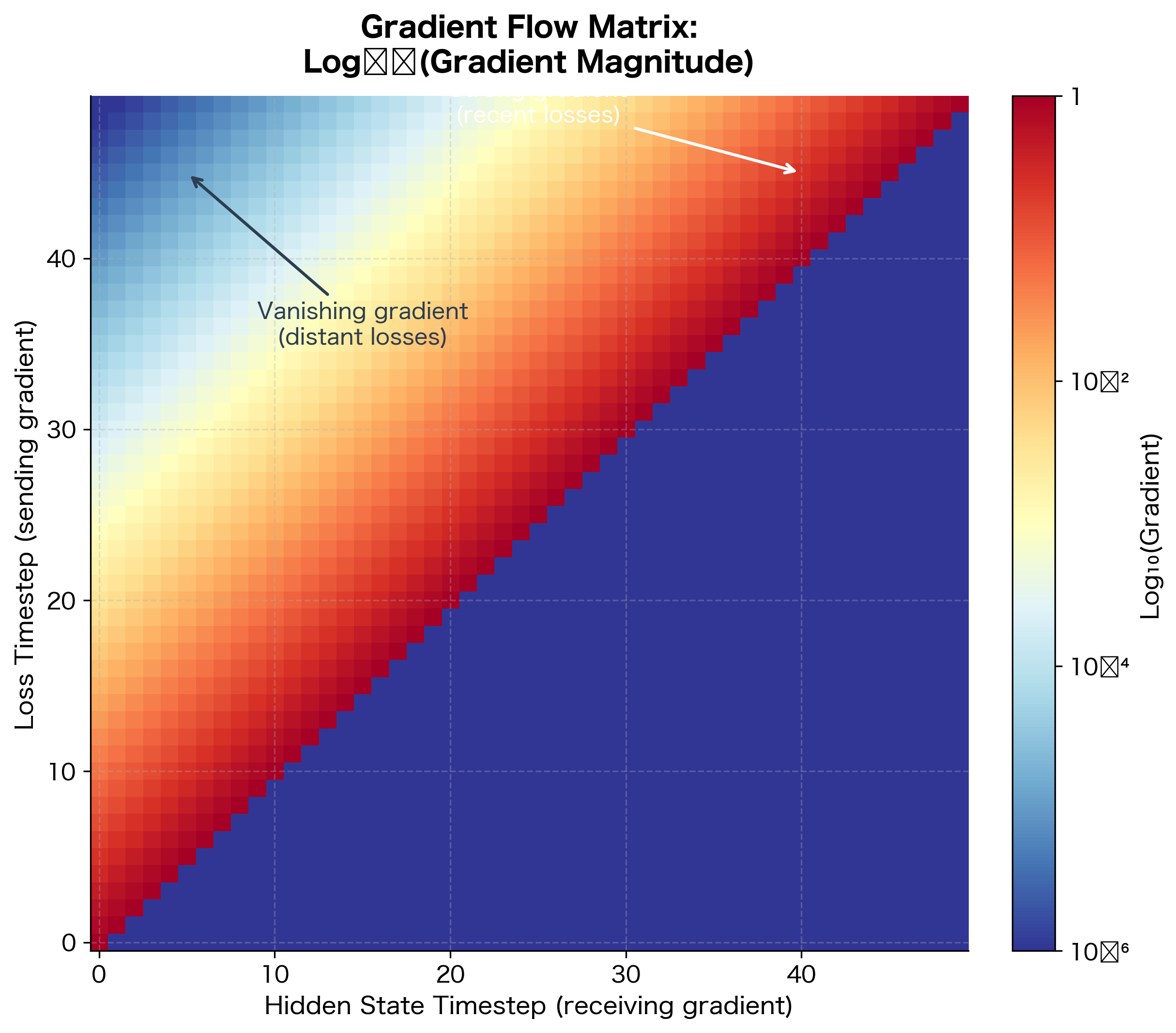
The heatmap makes the vanishing gradient problem visually stark. Each row represents a loss at a specific timestep; each column represents a hidden state that might need to be updated. The diagonal is bright (recent losses strongly affect recent hidden states), but the lower-left is dark (late losses barely affect early hidden states). If the correct prediction at timestep 50 depends on information from timestep 5, the gradient signal is attenuated by a factor of $0.75^{45} \approx 10^{-6}$, essentially zero for practical purposes.

The opposite problem, exploding gradients, occurs when the repeated multiplications amplify rather than shrink the gradient. The gradient grows exponentially, leading to numerical overflow and unstable training. Gradient clipping (limiting gradient magnitudes) provides a practical workaround, but it doesn't solve the underlying issue of gradient instability.

BPTT is inherently sequential. We must compute the forward pass through all timesteps before starting the backward pass, and the backward pass must proceed in reverse order. This sequential dependency prevents parallelization across timesteps, making RNN training slow compared to feedforward networks of similar depth.

Despite these limitations, BPTT was transformative. Before BPTT, training recurrent networks was largely impractical. BPTT made it possible to train networks that could:

• Model sequential dependencies in text, speech, and time series
• Learn from variable-length inputs without fixed-size windows
• Capture patterns that span multiple timesteps

The limitations of vanilla BPTT directly motivated architectural innovations. LSTMs and GRUs, which we'll cover in upcoming chapters, were designed specifically to address the vanishing gradient problem by creating "highways" for gradient flow. More recently, transformers abandoned recurrence entirely, using attention mechanisms that allow direct connections between any two positions in a sequence.

Understanding BPTT deeply, including its failure modes, is essential for appreciating why these newer architectures were developed and how they solve the problems that BPTT exposed.

This chapter derived and implemented Backpropagation Through Time, the algorithm that makes training recurrent neural networks possible.

The key concepts are:

• Unrolling: Conceptually unfold the RNN across time, treating it as a deep feedforward network with shared weights. This allows us to apply the chain rule systematically.

• Recursive gradient computation: The gradient at each hidden state combines the local loss gradient with the gradient flowing back from future timesteps: $\delta_t = \frac{\partial L_t}{\partial h_t} + \delta_{t+1} \cdot \frac{\partial h_{t+1}}{\partial h_t}$

• Gradient accumulation: Since weights are shared across timesteps, we sum gradient contributions from all timesteps. This is the defining characteristic of BPTT compared to standard backpropagation.

• Memory-computation trade-off: Full BPTT requires storing all hidden states, with memory scaling as $O(T \cdot d_h)$. Truncated BPTT reduces memory by limiting how far back gradients flow, at the cost of not learning very long-range dependencies.

• Gradient instability: The repeated multiplication of gradients through time leads to vanishing or exploding gradients, fundamentally limiting what vanilla RNNs can learn.

In the next chapter, we'll dive deeper into the vanishing gradient problem: why it occurs mathematically, how to visualize it, and why it motivated the development of gated architectures like LSTMs and GRUs.

When implementing BPTT, several parameters significantly affect training behavior and memory usage:

• hidden_size: The dimension of the hidden state vector. Larger values increase model capacity but also increase memory requirements quadratically (due to $\mathbf{W}_{hh}$ being $d_h \times d_h$). Typical values range from 128 to 1024.

• learning_rate: Controls the step size during gradient descent. RNNs are often sensitive to learning rate; values between 0.001 and 0.1 are common starting points. Too high causes instability; too low causes slow convergence.

• gradient_clip_value: The maximum allowed gradient magnitude. Clipping gradients to values like 1.0 or 5.0 prevents exploding gradients from destabilizing training, though it doesn't address vanishing gradients.

• truncation_length (k): For truncated BPTT, the number of timesteps to backpropagate through. Larger values capture longer dependencies but require more memory. Values of 20-50 are common; the optimal choice depends on the temporal structure of your data.

• weight_scale: The standard deviation for weight initialization. Small values (0.01-0.1) prevent initial activations from saturating, which would immediately cause vanishing gradients.

Ready to test your understanding? Take this quick quiz to reinforce what you've learned about Backpropagation Through Time.