

Master LSTM architecture including cell state, gates, and gradient flow. Learn how LSTMs solve the vanishing gradient problem with practical PyTorch examples.

This article is part of the free-to-read Language AI Handbook
Choose your expertise level to adjust how many terms are explained. Beginners see more tooltips, experts see fewer to maintain reading flow. Hover over underlined terms for instant definitions.
LSTM Architecture
In the previous chapter, we saw how vanilla RNNs struggle with long sequences. Gradients either vanish into insignificance or explode beyond control, making it nearly impossible to learn dependencies that span more than a few timesteps. This limitation motivated researchers to rethink the fundamental architecture of recurrent networks.
Long Short-Term Memory (LSTM) networks, introduced by Hochreiter and Schmidhuber in 1997, solve the vanishing gradient problem. The key insight is simple: instead of forcing information to pass through repeated nonlinear transformations at every timestep, create a dedicated pathway where information can flow unchanged across many timesteps. This "memory highway" allows LSTMs to maintain and access information over hundreds or even thousands of steps, enabling applications that were previously impossible with vanilla RNNs.
The Cell State: An Information Highway
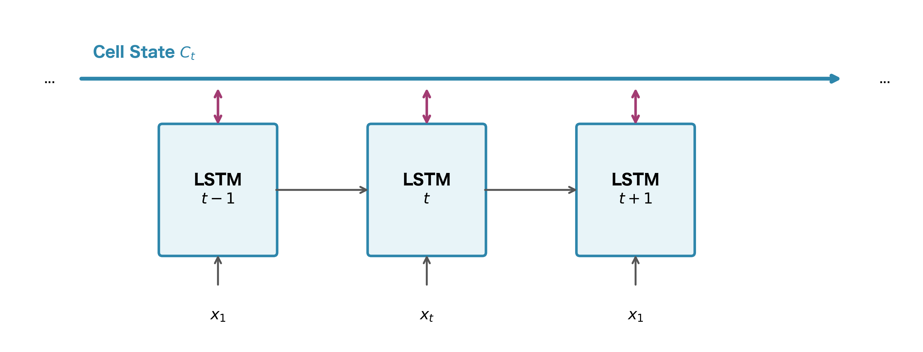
The defining feature of an LSTM is its cell state, a separate memory channel that runs parallel to the hidden state. Think of it as a conveyor belt that carries information through time. Unlike the hidden state in vanilla RNNs, which gets completely rewritten at each timestep, the cell state can preserve information indefinitely by simply passing it forward unchanged.
In a vanilla RNN, information at timestep must pass through every intermediate hidden state to reach timestep . Each passage involves a matrix multiplication and a tanh activation, which compresses values and causes gradients to shrink. After enough steps, the original signal is lost in the noise.
The cell state sidesteps this problem entirely. Information stored in the cell state can theoretically travel from the beginning to the end of a sequence with minimal transformation. The only operations applied to the cell state are element-wise additions and multiplications, both of which have well-behaved gradients that don't vanish or explode as readily as matrix multiplications through tanh.
LSTMs maintain two separate state vectors at each timestep :
- : the cell state, which stores long-term memory and flows through time with minimal modification
- : the hidden state, which is the output at each timestep and gets transformed more aggressively
The hidden state is what you typically use for predictions, but the cell state is what enables long-range learning.
Gate Mechanism Intuition
If the cell state were completely static, it would be useless. We need a way to selectively add new information, remove outdated information, and control what gets output. LSTMs accomplish this through gates, which are learned neural network layers that output values between 0 and 1.
Think of gates as dimmer switches rather than on/off toggles. A gate value of 0.0 means "block everything," 0.5 means "let half through," and 1.0 means "let everything through." Because gates use sigmoid activations, their outputs are always in this [0, 1] range, making them perfect for controlling information flow.
![Sigmoid activation function outputs values in [0, 1], making it ideal for gates that control information flow. Values near 0 block information, values near 1 pass it through.](https://cnassets.uk/notebooks/4_lstm_architecture_files/sigmoid-activation-function.png)
![Tanh activation function outputs values in [-1, 1], allowing candidate values to both increase and decrease cell state elements. The symmetric range around zero enables bidirectional updates.](https://cnassets.uk/notebooks/4_lstm_architecture_files/tanh-activation-function.png)
LSTMs have three gates, each serving a distinct purpose:
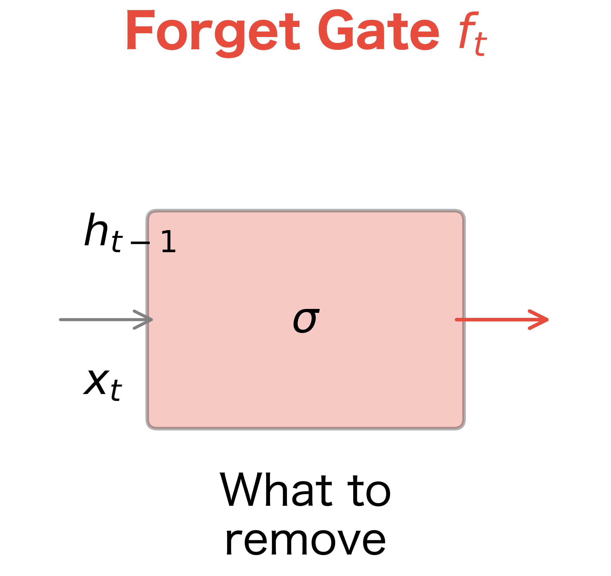
- Forget gate: Decides what information to discard from the cell state. When processing a new sentence, you might want to forget the subject of the previous sentence.
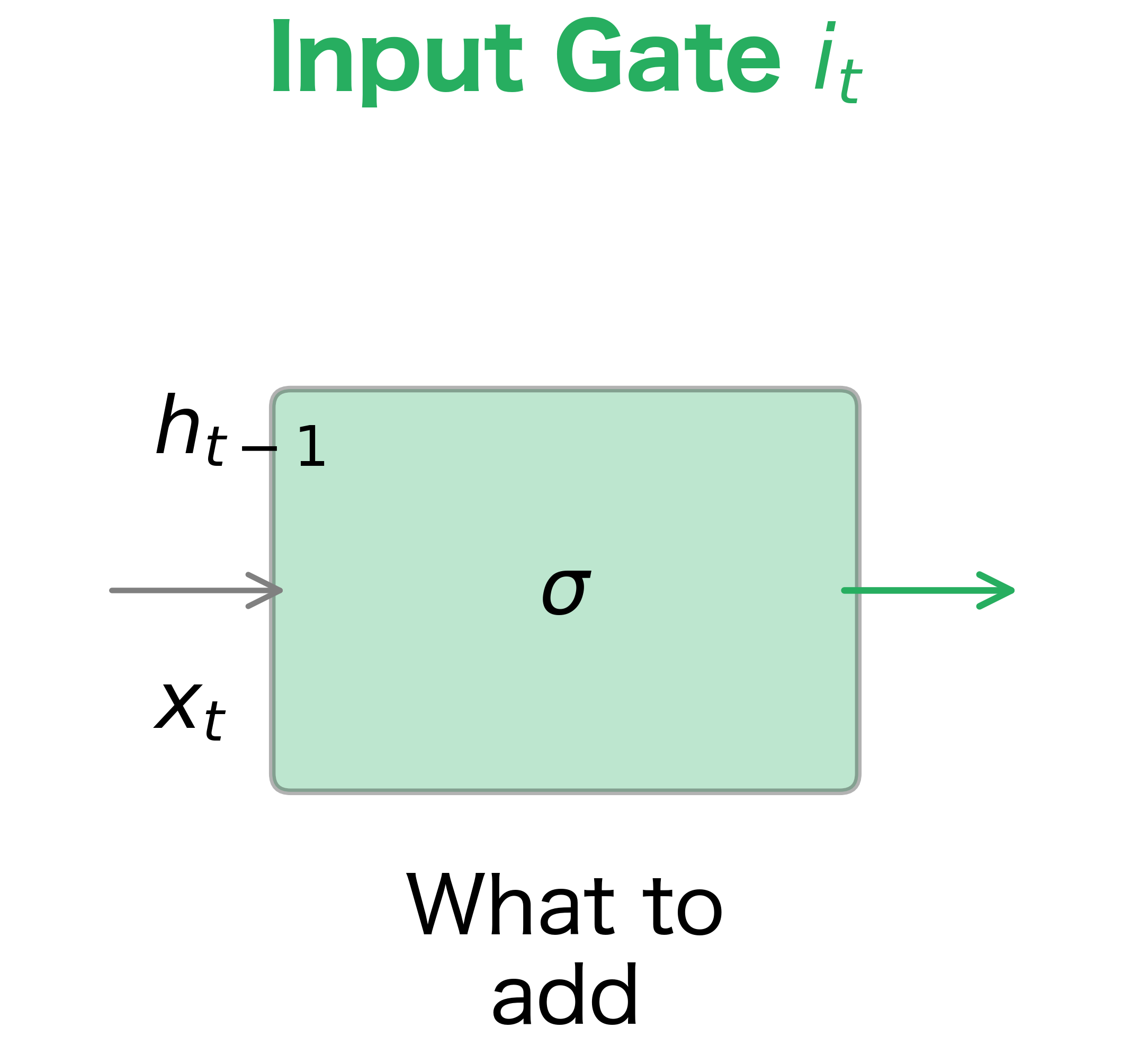
- Input gate: Decides what new information to store in the cell state. When you encounter a new subject, you want to remember it.
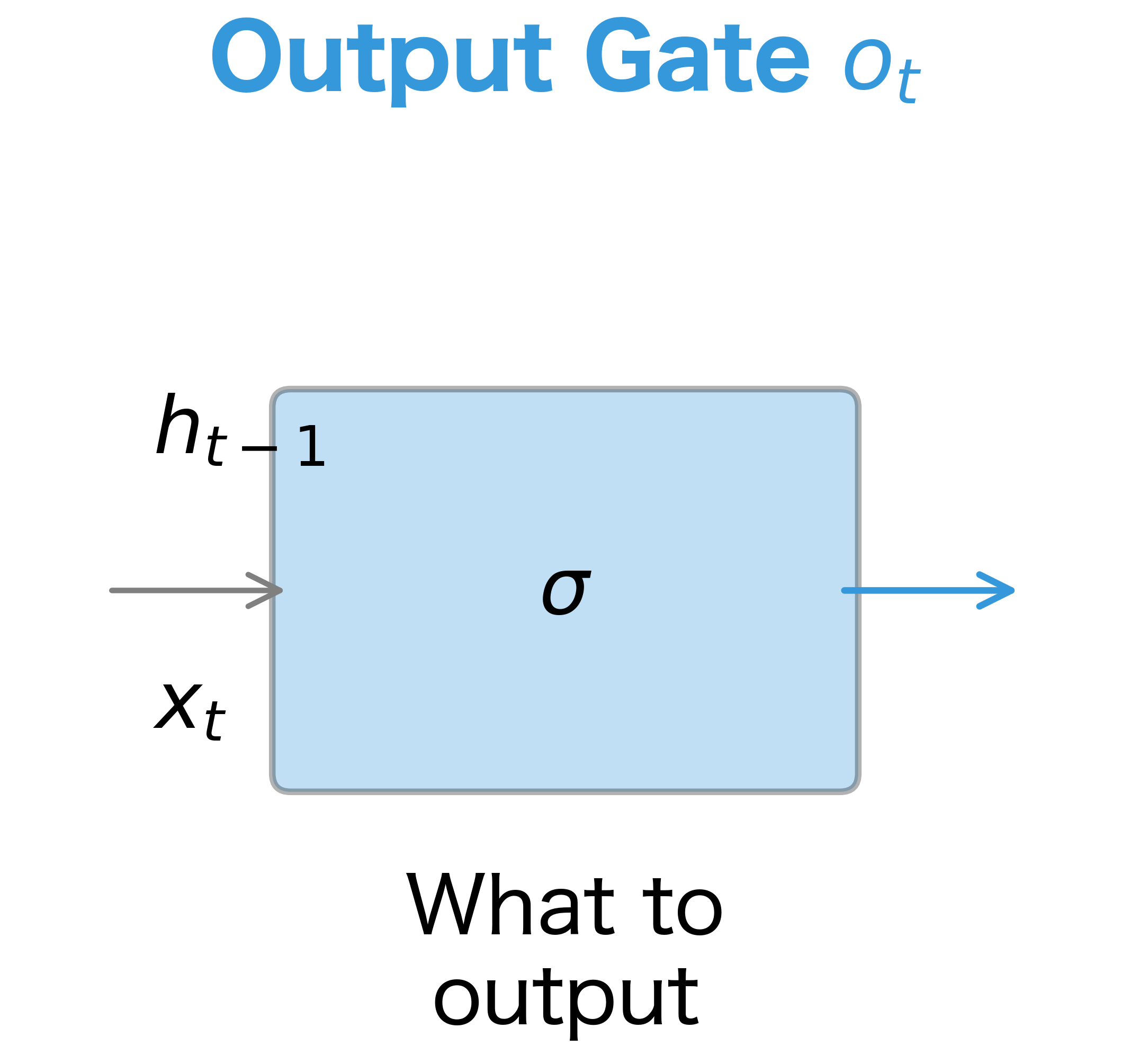
- Output gate: Decides what part of the cell state to output as the hidden state. Not everything you remember is relevant to the current prediction.
Each gate takes the same inputs: the previous hidden state and the current input . The gate computation follows the same pattern for all three gates:
where:
- : the sigmoid activation function, which outputs values in
- : the weight matrix for this gate (each gate has its own weights)
- : the concatenation of the previous hidden state and current input
- : the bias vector for this gate
Each gate learns different weights, allowing it to specialize in its particular function. The forget gate might learn to reset memory when it sees a period, while the input gate might learn to store information when it sees a noun.
LSTM Diagram Walkthrough
Now that we understand what gates do conceptually, let's see how they work together to create a complete memory system. The LSTM cell coordinates forgetting, remembering, and outputting, all happening simultaneously at each timestep. Understanding this coordination is key to understanding why LSTMs work so well.
The diagram below shows a single LSTM cell, which gets replicated at each timestep with shared weights. Follow the information flow from left to right: the cell state runs along the top like a highway, while the hidden state flows along the bottom. The gates act as on-ramps and off-ramps, controlling what enters and exits this memory highway.
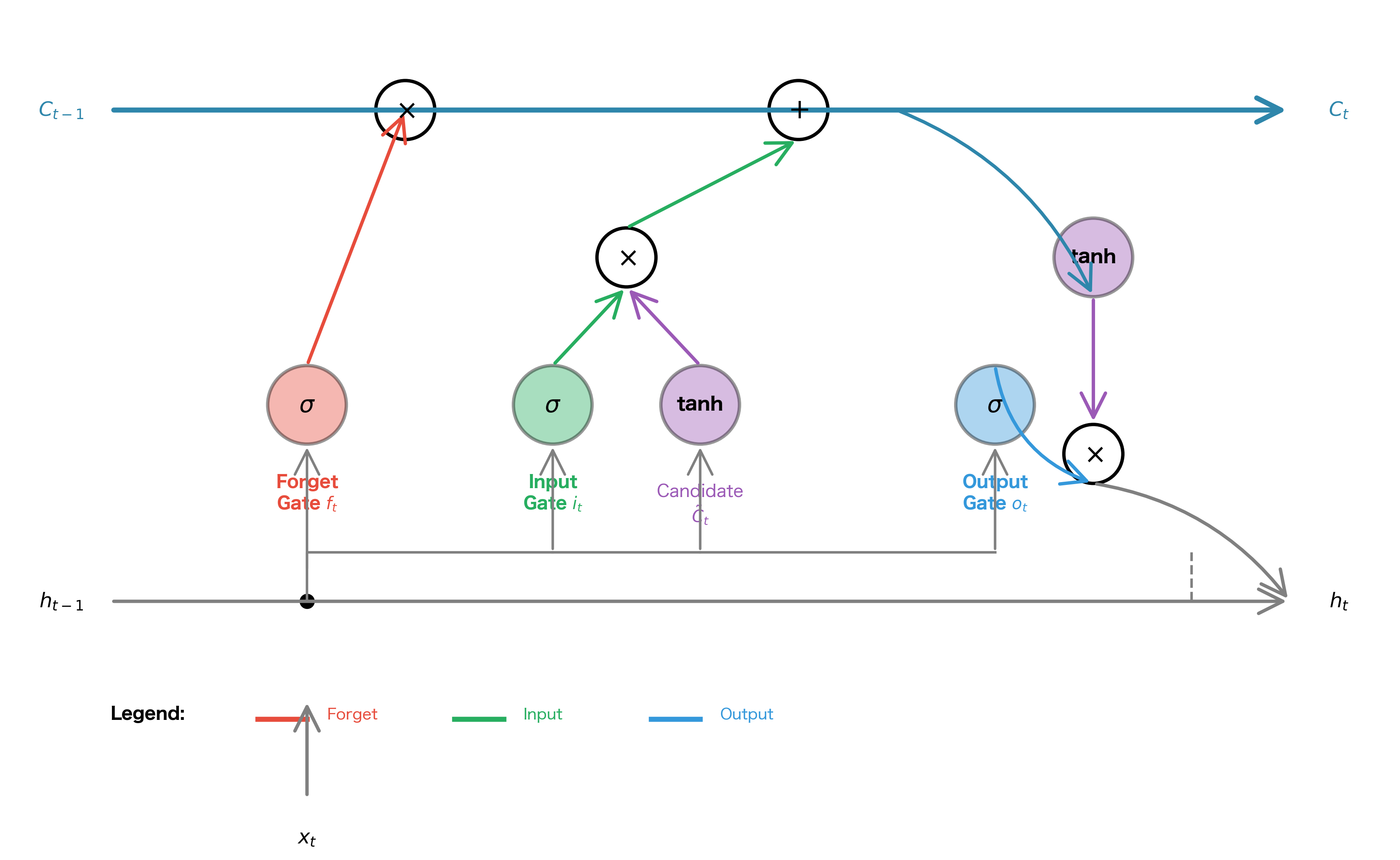
The Four Stages of LSTM Processing
The LSTM cell processes information in four distinct stages, each building on the previous. Think of it as a careful decision-making process: first decide what old information to discard, then decide what new information to add, then actually update the memory, and finally decide what to output. Let's walk through each stage.
Stage 1: The Forget Gate Decides What to Discard
Before we can add new information, we need to make room by discarding irrelevant old information. The forget gate examines the previous hidden state and current input , asking: "Given what I just saw, what should I forget from my long-term memory?"
The forget gate computes:
where:
- : the forget gate output, a vector with one value per cell state element
- : the forget gate's weight matrix
- : concatenation of previous hidden state and current input
- : the forget gate's bias vector
- : the sigmoid function, ensuring outputs fall in
The sigmoid activation is crucial here. It produces values between 0 and 1, which act as "retention percentages" for each element of the cell state. A value of 0.1 means "keep only 10% of this information," while 0.95 means "keep almost all of it." The network learns these retention patterns during training.
Stage 2: The Input Gate and Candidate Values
With forgetting handled, we turn to remembering. This stage involves two parallel computations that work together: the input gate decides which cell state elements to update, while a tanh layer creates candidate values that could be added.
The input gate computes:
Simultaneously, we create candidate values:
where:
- : the input gate output, controlling which elements to update
- : candidate values that could be added to the cell state
- : separate weight matrices for the input gate and candidate computation
- : corresponding bias vectors
Why use tanh for the candidates? The tanh function outputs values in , allowing the network to both increase and decrease cell state values. A candidate of +0.8 would push the cell state up, while -0.8 would push it down. The input gate then scales these candidates, determining how much of each proposed change to actually apply.
Stage 3: The Cell State Update
Now comes the core of the LSTM: the actual memory update. We combine the forgetting and remembering decisions into a single formula:
where:
- : the new cell state at timestep
- : the previous cell state from timestep
- : the forget gate output, controlling retention of old information
- : the input gate output, controlling addition of new information
- : the candidate values to potentially add
- : element-wise (Hadamard) multiplication
This formula looks simple but does a lot. The first term, , selectively preserves old information. If for some element , we keep 90% of that element's previous value. The second term, , selectively adds new information. If and , we add to that element.
Notice that this is an additive update, not a multiplicative one like in vanilla RNNs. This additive structure is the key to solving the vanishing gradient problem: gradients can flow backward through the addition operation without being repeatedly multiplied by small values.
Let's visualize this update with concrete numbers. Suppose we have a 4-dimensional cell state and the network has computed specific gate values:
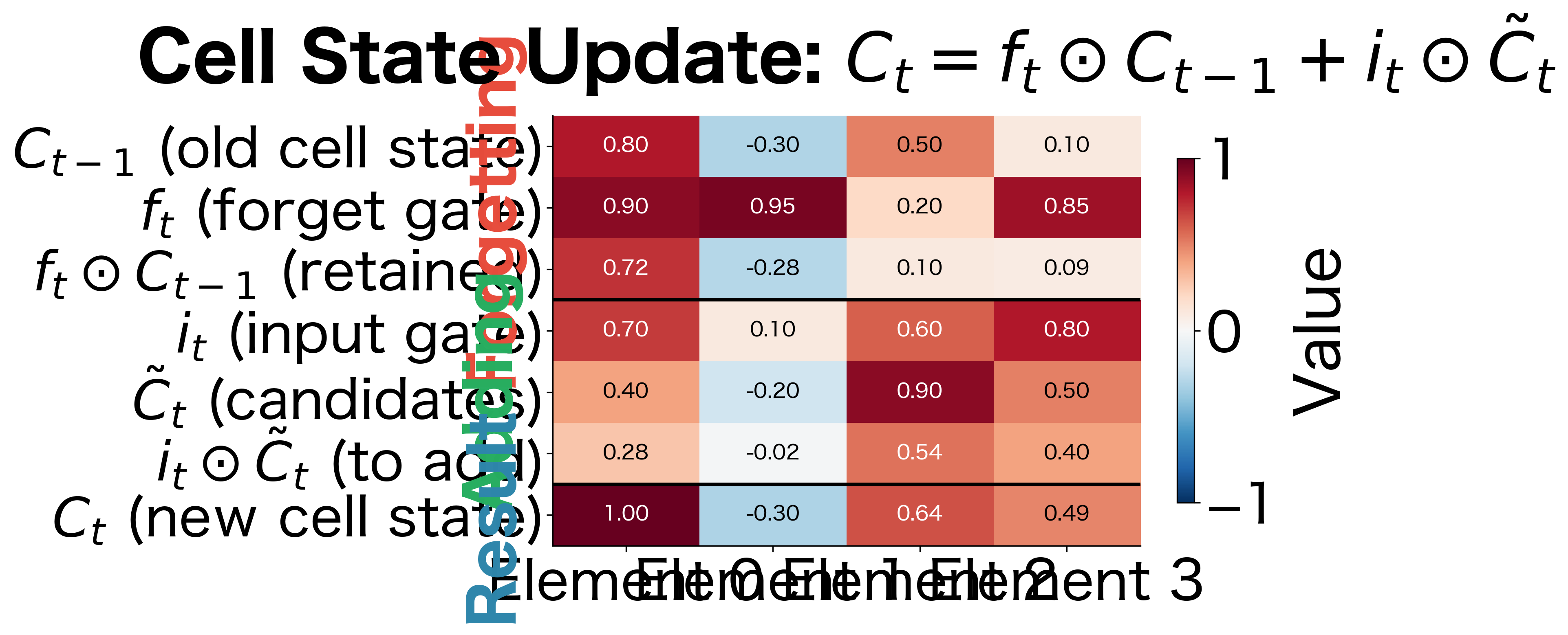
In this example, notice how element 2 behaves differently from the others. The forget gate value of 0.2 means we discard 80% of the old information in that position, while the input gate value of 0.6 means we add a substantial portion of the candidate value 0.9. The result is that element 2 shifts from 0.5 to 0.64, dominated by the new information rather than the old.
Stage 4: The Output Gate Produces the Hidden State
The cell state now contains our updated long-term memory, but not all of it is relevant to the current timestep's output. The output gate filters the cell state to produce the hidden state:
where:
- : the output gate, controlling which cell state elements to expose
- : the hidden state output at timestep
- : the cell state squashed to
The tanh applied to the cell state serves two purposes. First, it bounds the values to a reasonable range, preventing any single element from dominating. Second, it centers the values around zero, which tends to help with downstream computations. The output gate then selects which of these bounded values to include in the hidden state.
This hidden state serves dual purposes: it's the output that downstream layers or predictions use, and it's also fed back into the LSTM at the next timestep as . This recurrence is what makes the network "recurrent," allowing information to persist across time.
Putting It All Together
The complete LSTM computation at each timestep can be summarized as:
- Forget:
- Input gate:
- Candidate:
- Cell update:
- Output gate:
- Hidden state:
Each gate learns its own weight matrix and bias, giving the network four sets of parameters to learn: , , , and . During training, backpropagation adjusts these parameters so that the gates learn to open and close at the right times for the task at hand.
Information Flow in LSTMs
Understanding how information flows through an LSTM is crucial for building intuition about what these networks can learn. Let's trace a concrete example.
Consider processing the sentence: "The cat, which had been sleeping on the warm windowsill since early morning, finally stretched." The subject "cat" appears at the beginning, but the verb "stretched" doesn't appear until the end. A vanilla RNN would struggle to connect these, but an LSTM can maintain the subject in its cell state throughout.
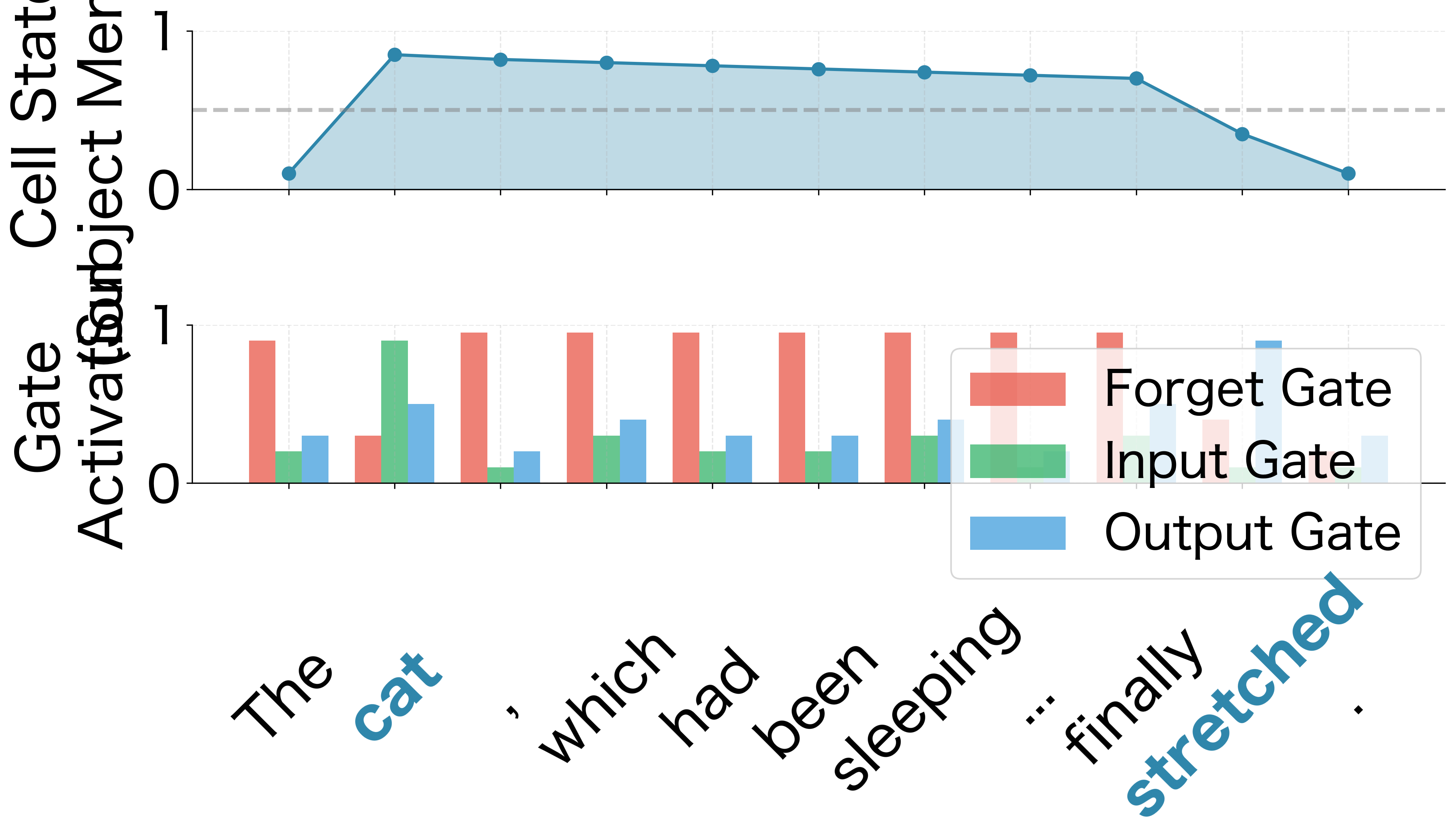
When the LSTM encounters "cat," the input gate activates strongly, storing the subject information in the cell state. The forget gate stays relatively open (high values), preserving this information. As the network processes the intervening clause "which had been sleeping on the warm windowsill since early morning," the forget gate remains high, maintaining the subject memory. Other information might be added and removed, but the subject slot stays protected.
When "stretched" arrives, the output gate activates strongly, allowing the stored subject information to influence the prediction. The model can now correctly associate "cat" with "stretched" despite the many intervening words.
LSTMs for Long Sequences
The advantage of LSTMs becomes clear when we compare their performance to vanilla RNNs on sequences of varying lengths. Let's visualize how gradient magnitude changes across sequence length for both architectures.
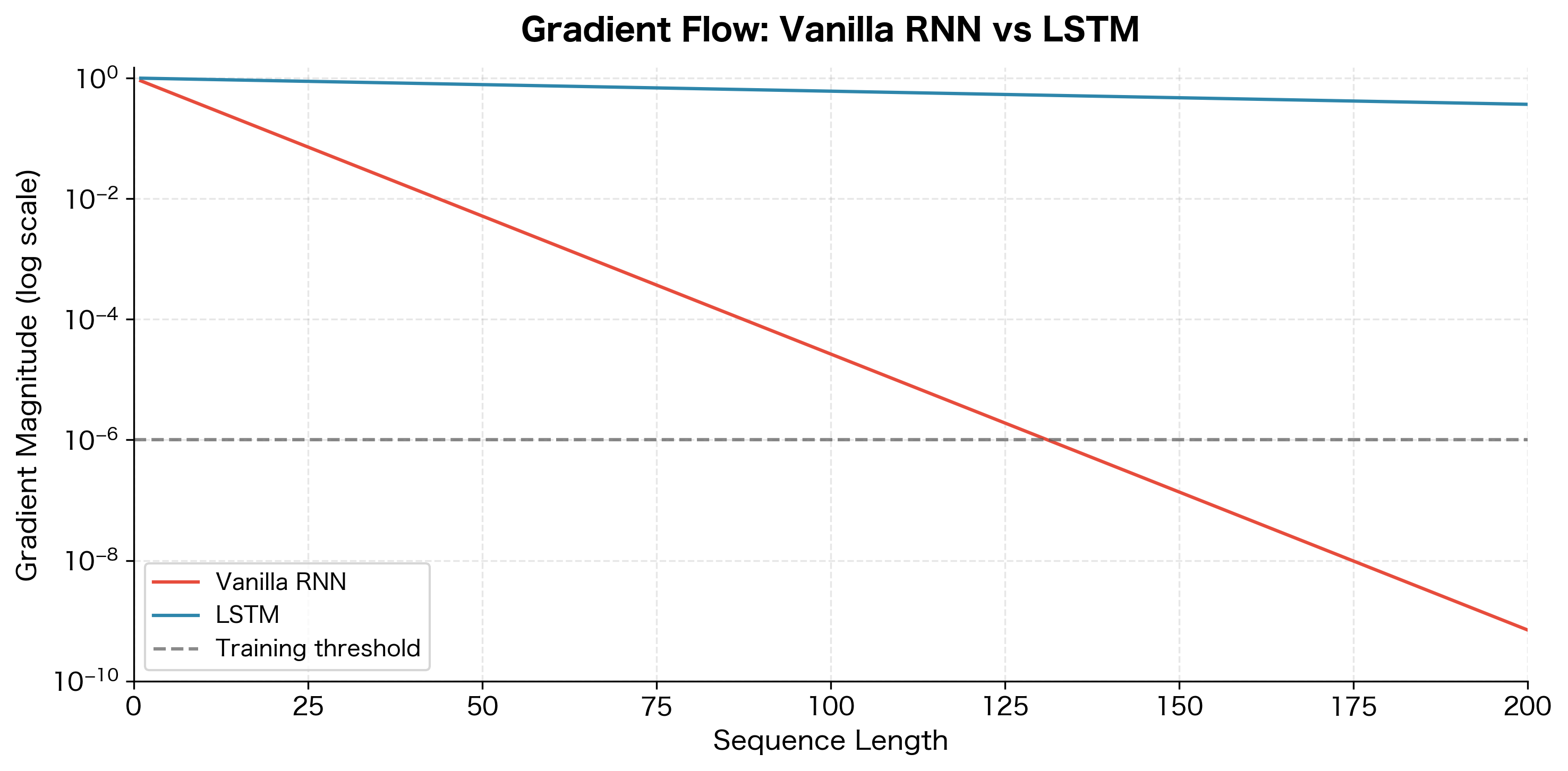
The difference is substantial. Vanilla RNN gradients become negligible after around 50 timesteps, making it impossible to learn dependencies beyond that range. LSTM gradients, while still decaying, remain orders of magnitude larger and stay above practical training thresholds for much longer sequences.
This gradient stability translates directly into learning capability. LSTMs can learn to copy information, detect patterns, and make predictions that depend on inputs hundreds of timesteps in the past. Tasks like language modeling, machine translation, and speech recognition all benefit from this extended memory.
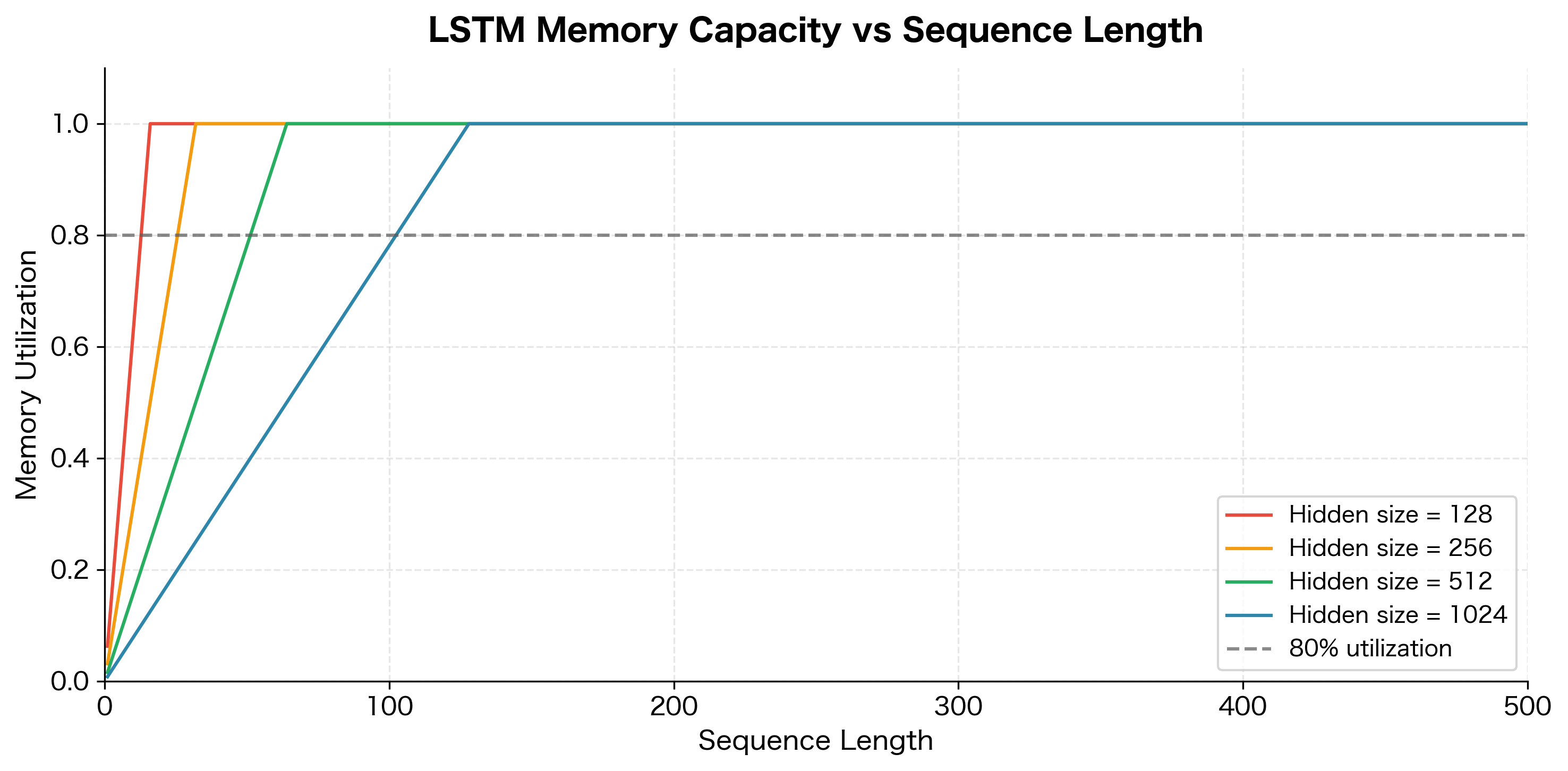
LSTM Memory Capacity
While LSTMs can theoretically maintain information indefinitely, their practical memory capacity is finite. The cell state has a fixed dimensionality, typically between 128 and 1024 units, and each unit can only store a limited amount of information. As sequences grow longer and more complex, the network must decide what to remember and what to forget.
Several factors affect how efficiently an LSTM uses its memory capacity:
- Task complexity: Simple pattern matching requires less memory than complex reasoning. Copying a sequence verbatim is easier than understanding and summarizing it.
- Information redundancy: Natural language has significant redundancy. An LSTM doesn't need to store every word verbatim; it can store compressed representations.
- Forgetting strategy: A well-trained forget gate learns to discard irrelevant information, freeing up capacity for what matters.
- Hidden size: Larger hidden dimensions provide more storage but also require more computation and training data.
In practice, standard LSTMs work well for sequences up to a few hundred tokens. Beyond that, you'll need architectural modifications like attention mechanisms (which we'll cover in later chapters) or hierarchical structures that process long documents in chunks.
Comparing LSTM and Vanilla RNN
Theory is valuable, but seeing the difference in practice makes it concrete. Let's design an experiment that directly tests the core claim: LSTMs can remember information across long distances where vanilla RNNs fail.
Designing the Memory Task
We need a task that isolates memory ability from other confounding factors. The simplest such task is a "delayed recall" problem: show the model a signal at some position in a sequence, fill the rest with noise, and ask it to recall what the signal was at the end. The longer the delay between signal and recall, the harder the task becomes for architectures with poor long-term memory.
Concretely, our task works as follows:
- Generate a sequence of length 110 timesteps
- Place a one-hot signal (one of 8 possible classes) at a specific position
- Fill all other positions with random noise
- Train the model to predict which class the signal belonged to
If the signal is placed 5 timesteps before the end, the model only needs to remember for 5 steps. If placed 100 timesteps before the end, it must remember across 100 steps of noise. This clean setup lets us measure exactly how memory degrades with distance.
Implementing the Models
First, we define both model architectures using PyTorch. Notice how similar the code is: the only difference is that nn.LSTM returns both a hidden state and a cell state, while nn.RNN only returns a hidden state. This similarity makes the performance difference even more notable.
Data Generation and Training
Next, we implement the data generation and training functions. The signal_position parameter controls how far back the model must remember, which directly determines the task difficulty.
Running the Experiment
Now we run the experiment, testing both architectures across memory distances from 5 to 100 timesteps. For each distance, we train a fresh model for 100 epochs and measure its final accuracy. This gives us a direct comparison of how each architecture handles increasing memory demands.
The results show a clear difference between the two architectures:
At short distances (5-10 timesteps), both models perform reasonably well. But as the memory distance increases, the vanilla RNN's accuracy drops toward random chance, while the LSTM maintains strong performance even at 100 timesteps. This pattern directly reflects the vanishing gradient problem: the vanilla RNN simply cannot propagate learning signals across long distances.
Interpreting the Results
The results show the LSTM's advantage clearly. The vanilla RNN's accuracy drops to near-random chance (12.5% for 8 classes) as the memory distance increases beyond 20-30 timesteps. The LSTM, by contrast, maintains high accuracy even when the signal is 100 timesteps away from the output.
This isn't a subtle difference. It's a fundamental capability gap. The vanilla RNN literally cannot learn to solve this task at long distances, no matter how long you train it. The gradients that would teach it to connect the signal to the output simply vanish before they reach the relevant timesteps.
The LSTM succeeds because of the architectural innovations we've discussed: the cell state provides an unobstructed gradient highway, and the gates learn to protect the signal information from being overwritten by noise. This is exactly the kind of long-range dependency that makes LSTMs so valuable for real-world sequence tasks like language modeling, machine translation, and speech recognition.
Limitations and Impact
The LSTM architecture has limitations worth understanding. Knowing these constraints helps you decide when to use LSTMs and when to consider alternatives.
The most significant practical limitation is computational cost. LSTMs are inherently sequential: you cannot compute the hidden state at timestep until you've computed the hidden state at timestep . This sequential dependency prevents parallelization across timesteps, making LSTMs slow to train on long sequences compared to architectures like Transformers that can process all positions simultaneously. On modern GPUs optimized for parallel computation, this sequential bottleneck becomes increasingly painful as sequence lengths grow.
Memory requirements also scale linearly with sequence length during training. Backpropagation through time requires storing all intermediate hidden states and cell states, which can exhaust GPU memory for very long sequences. Techniques like truncated backpropagation help, but they sacrifice the ability to learn the longest-range dependencies.
Despite these limitations, LSTMs changed how we approach sequence modeling. Before LSTMs, neural networks struggled with any task requiring memory beyond a few timesteps. After LSTMs, machine translation, speech recognition, handwriting recognition, and countless other sequence tasks became tractable. The key insight of creating a protected memory pathway with learned gating has influenced virtually every subsequent sequence architecture.
LSTMs also introduced the concept of gating mechanisms to the broader deep learning community. The idea that neural networks could learn to dynamically control information flow, rather than simply transforming it, opened new research directions. Attention mechanisms, which now dominate NLP, can be seen as a generalization of the gating concept: instead of learning fixed gates, attention learns dynamic, content-dependent gates over the entire sequence.
Summary
This chapter introduced the LSTM architecture and its key innovations for processing sequences with long-range dependencies.
The central insight behind LSTMs is the cell state, an information highway that allows data to flow through time with minimal transformation. Unlike the hidden state in vanilla RNNs, which gets completely overwritten at each timestep, the cell state can preserve information indefinitely through additive updates.
Three learned gates control information flow through the LSTM:
- The forget gate decides what information to discard from the cell state
- The input gate decides what new information to store
- The output gate decides what part of the cell state to expose as output
These gates enable LSTMs to selectively remember, update, and retrieve information based on the input and context. The result is stable gradient flow during training, allowing LSTMs to learn dependencies spanning hundreds of timesteps.
In the next chapter, we'll dive into the mathematical details of LSTM gate equations, deriving each component and implementing an LSTM from scratch. Understanding the precise computations will deepen your intuition for how these networks learn to manage memory.
Key Parameters
When working with LSTMs in PyTorch (nn.LSTM), several parameters significantly impact model behavior:
- hidden_size: The dimensionality of the hidden state and cell state vectors. Larger values (256-1024) provide more memory capacity but increase computation. Start with 128-256 for most tasks.
- num_layers: Number of stacked LSTM layers. Deeper networks (2-4 layers) can learn more complex patterns but are harder to train. Single-layer LSTMs often suffice for many sequence tasks.
- batch_first: When
True, input tensors have shape(batch, seq_len, features). WhenFalse(default), shape is(seq_len, batch, features). Usingbatch_first=Truealigns with common data loading patterns. - dropout: Dropout probability applied between LSTM layers (only active when
num_layers > 1). Values of 0.1-0.3 help prevent overfitting on longer sequences. - bidirectional: When
True, runs the LSTM in both forward and backward directions, doubling the hidden state size. Useful for tasks where future context matters (e.g., classification), but not applicable for generation tasks.
Quiz
Ready to test your understanding? Take this quick quiz to reinforce what you've learned about LSTM architecture and how it solves the vanishing gradient problem.

Comments