

Learn the encoder-decoder framework for sequence-to-sequence learning, including context vectors, LSTM implementations, and the bottleneck problem that motivated attention mechanisms.

This article is part of the free-to-read Language AI Handbook
Choose your expertise level to adjust how many terms are explained. Beginners see more tooltips, experts see fewer to maintain reading flow. Hover over underlined terms for instant definitions.
Encoder-Decoder Framework
In the previous part, we explored how recurrent neural networks process sequences, capturing temporal dependencies through hidden states that accumulate information over time. But there's a fundamental limitation we haven't addressed: what if the input and output sequences have different lengths? How do you translate "The cat sat on the mat" (six words) into "Le chat était assis sur le tapis" (seven words)? How do you summarize a 500-word article into a 50-word abstract?
These variable-length sequence-to-sequence problems require a new architectural paradigm. The encoder-decoder framework, introduced by Sutskever et al. in 2014, provides an elegant solution: use one RNN to compress the input sequence into a fixed-size representation, then use another RNN to generate the output sequence from that representation. This simple idea unlocked machine translation, text summarization, and countless other applications that transform one sequence into another.
The Core Insight: Separate Reading from Writing
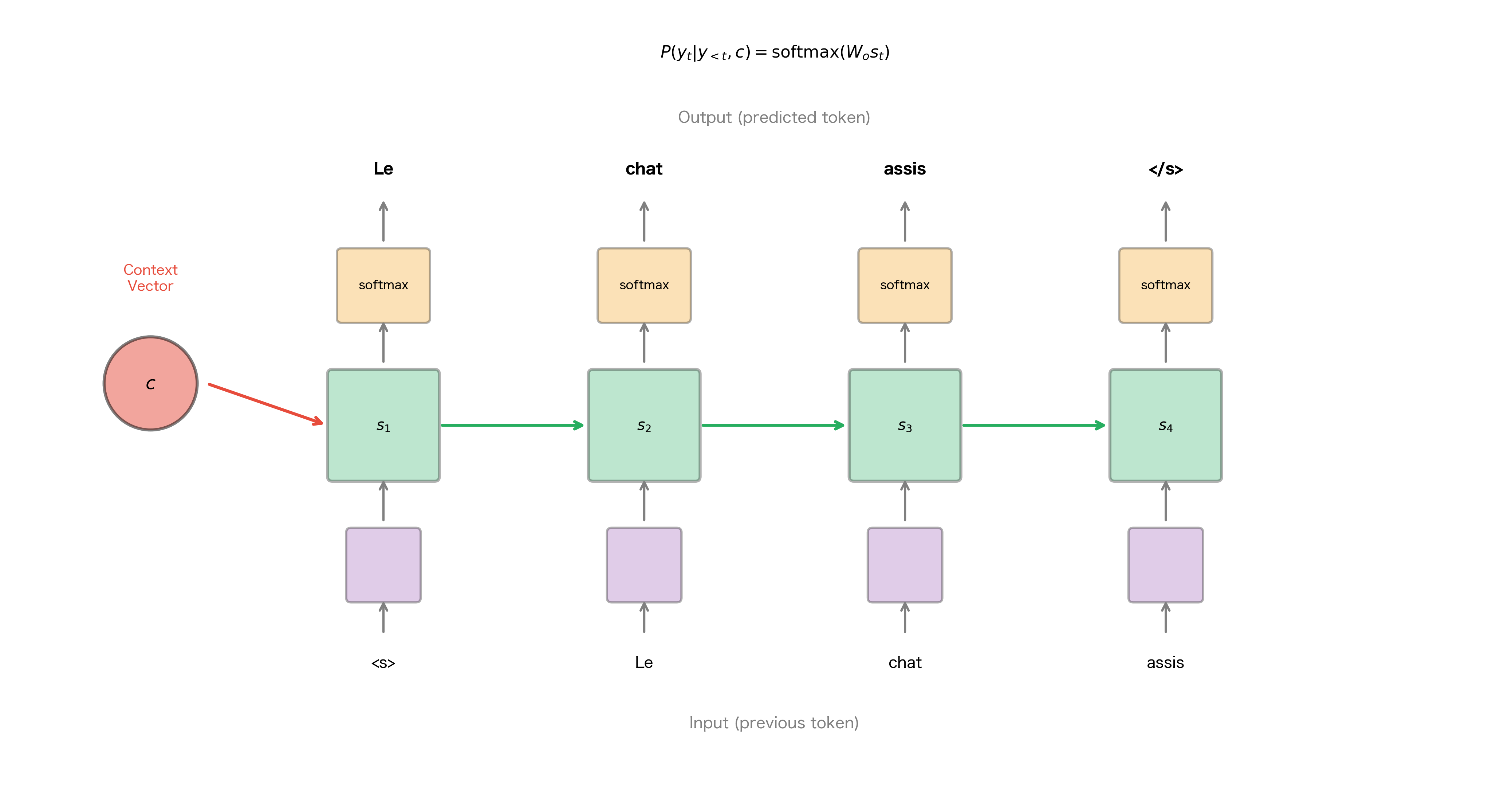
Before diving into architecture details, let's understand the fundamental insight behind encoder-decoder models. Consider how a human translator works. First, they read the entire source sentence, building a mental understanding of its meaning. Then, they produce the translation word by word, consulting their mental representation of the original. They don't translate word by word as they read, because that would fail to capture context and produce awkward, literal translations.
The encoder-decoder framework mirrors this process. The encoder "reads" the input sequence, compressing it into a dense vector representation called the context vector. The decoder then "writes" the output sequence, using the context vector as its guide. This separation allows each component to specialize: the encoder focuses on understanding, while the decoder focuses on generation.
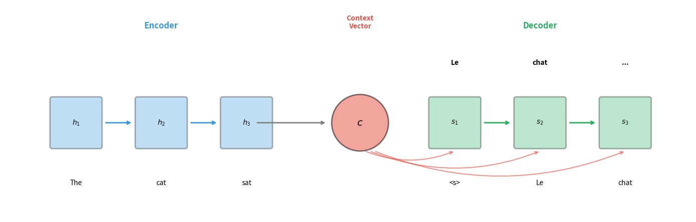
The figure illustrates the basic flow. The encoder processes "The cat sat" sequentially, with each hidden state incorporating information from all previous words. After processing the final word, the encoder's hidden state becomes the context vector . The decoder then generates the translation, starting with a special start token <s> and producing one word at a time until it outputs an end token.
The Encoder: Compressing Input into Meaning
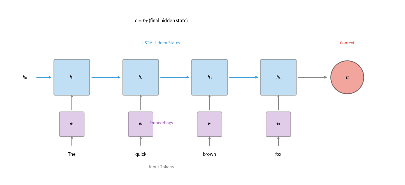
The encoder's job is straightforward: process the input sequence and produce a fixed-size representation that captures its meaning. We can use any RNN architecture for this purpose, whether vanilla RNN, LSTM, or GRU. In practice, LSTMs and GRUs dominate due to their ability to capture long-range dependencies.
Encoder Architecture
For an input sequence of length , the encoder computes a sequence of hidden states:
where:
- : the input token at timestep , typically represented as an embedding vector
- : the previous hidden state, carrying information from tokens
- : the new hidden state, now incorporating information from
- : the encoder's recurrent function (LSTM, GRU, etc.)
The final hidden state serves as the context vector , summarizing the entire input sequence in a single vector:
where:
- : the context vector that will be passed to the decoder
- : the encoder's hidden state after processing all input tokens
This is remarkably simple, but there's a subtle point worth emphasizing. The context vector must encode everything the decoder needs to know about the input. For a 100-word input sentence, all the semantic content, syntactic structure, and nuance must be compressed into a vector of perhaps 512 or 1024 dimensions. This compression is both the power and the limitation of the basic encoder-decoder framework.
Implementing the Encoder
Let's implement a basic LSTM encoder in PyTorch. The implementation is straightforward because PyTorch's nn.LSTM handles the sequential processing internally:
The encoder returns both the hidden state and cell state (for LSTM). These together form the context that initializes the decoder. Notice that we don't return the outputs tensor containing all hidden states. In the basic encoder-decoder framework, only the final hidden state matters. Later, when we add attention, we'll need those intermediate states.
The hidden state has shape (num_layers, batch_size, hidden_size). For a 2-layer LSTM, this means we have two hidden vectors per sequence: one from the first layer and one from the second. Both contribute to the context that initializes the decoder.
To visualize how information accumulates in the encoder, let's examine the hidden state activations as the encoder processes a sequence:
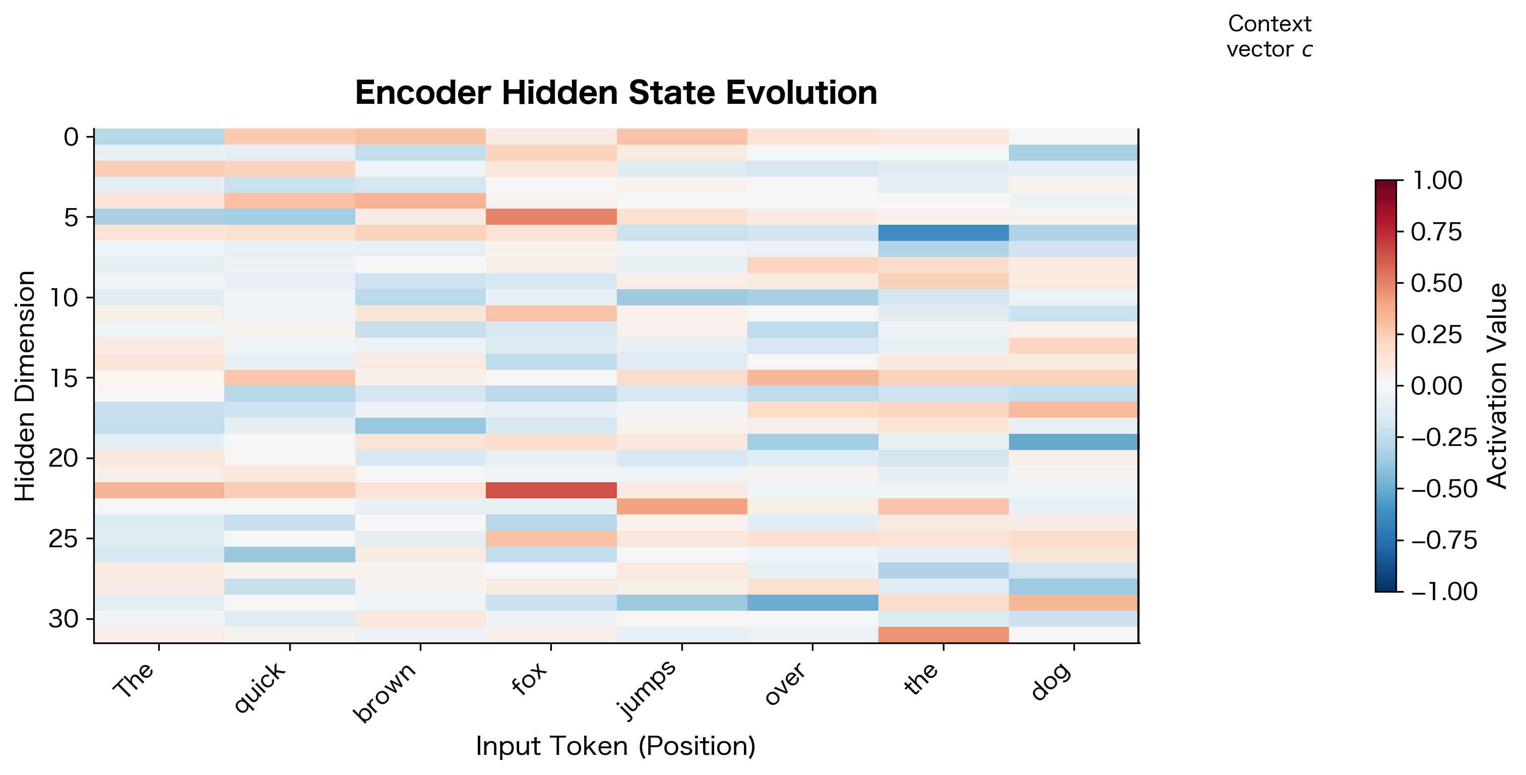
The heatmap reveals how the encoder builds up its representation. Each column shows the hidden state after processing one more token. Notice how the activation patterns change across positions: some dimensions respond strongly to specific words, while others accumulate information gradually. The rightmost column is the context vector that gets passed to the decoder. It must encode everything about the input sequence that the decoder needs for translation.
The Decoder: Generating Output from Context
The decoder's job is more complex than the encoder's. It must generate the output sequence one token at a time, where each token depends on the context vector and all previously generated tokens. This autoregressive generation creates a dependency chain: to generate token , you need tokens .
Decoder Architecture
The decoder is also an RNN, but with a crucial difference: its initial hidden state comes from the encoder's context vector rather than being initialized to zeros. At each timestep , the decoder:
- Takes the previous output token as input
- Updates its hidden state using the RNN
- Produces a probability distribution over the vocabulary
- Samples or selects the next token
Mathematically, the decoder performs two operations at each timestep. First, it updates its hidden state by combining the previous token with its memory of what it has generated so far:
where:
- : the decoder's hidden state at timestep , encoding information about all previously generated tokens
- : the embedding of the previous output token (or the start token
<s>when ) - : the decoder's hidden state from the previous timestep
- : the decoder's recurrent function (LSTM, GRU, etc.)
The crucial initialization is , meaning the decoder starts with the context vector from the encoder as its initial hidden state. This is how information flows from the encoder to the decoder.
Second, the decoder converts its hidden state into a probability distribution over the vocabulary to predict the next token:
where:
- : probability distribution over all vocabulary tokens for position
- : output projection weight matrix of shape (vocab_size, hidden_size)
- : the current decoder hidden state
- : output projection bias vector of shape (vocab_size,)
- : all previously generated tokens
- : the context vector (implicitly encoded in the hidden states through initialization)
The softmax function converts the raw scores (logits) into a valid probability distribution that sums to 1, allowing us to either sample from this distribution or take the most probable token.
To see this concretely, let's visualize what a typical decoder output looks like. The decoder produces a probability distribution over the entire vocabulary at each timestep:
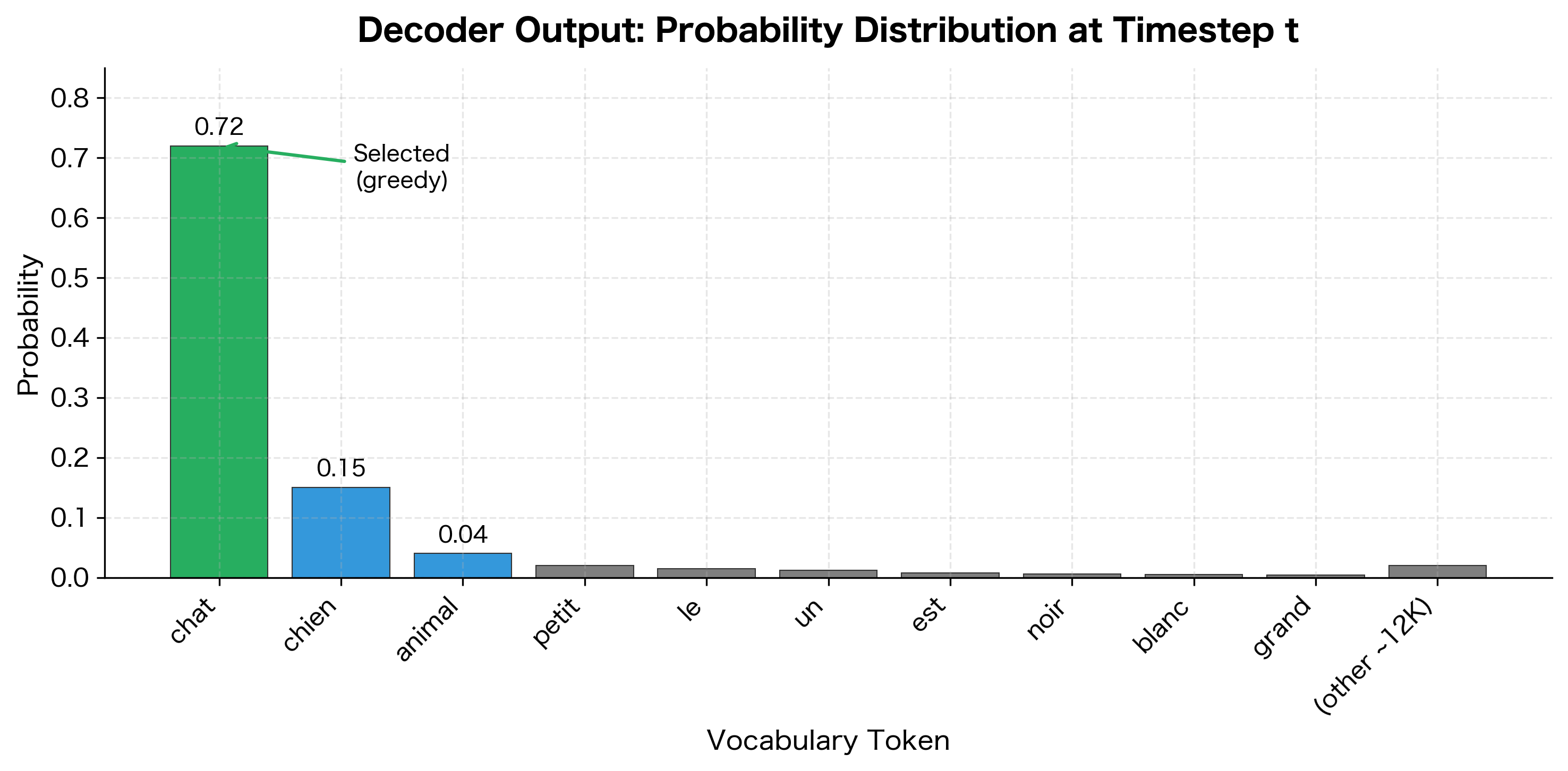
This visualization shows a typical decoder output. The model has learned that "chat" (cat) is the most likely next word given the context, assigning it 72% probability. Alternative translations like "chien" (dog) receive smaller but non-negligible probability. The long tail of the distribution spreads tiny probabilities across thousands of other vocabulary tokens.
Implementing the Decoder
The decoder implementation requires careful handling of the autoregressive generation process:
During training, we feed the entire target sequence to the decoder at once. This is called teacher forcing, which we'll cover in detail in the next chapter. The key insight is that during training, we know the correct output sequence, so we can compute all timesteps in parallel rather than generating one token at a time.
Connecting Encoder and Decoder: The Seq2Seq Model
Now let's combine the encoder and decoder into a complete sequence-to-sequence model:
The output has shape (batch_size, trg_len, vocab_size), containing unnormalized log-probabilities (logits) for each position in the target sequence. During training, we compute the cross-entropy loss between these predictions and the actual target tokens.
The Context Vector Bottleneck
The basic encoder-decoder architecture has a fundamental limitation: all information about the source sequence must pass through a single fixed-size context vector. This creates an information bottleneck that becomes increasingly problematic as sequences grow longer.
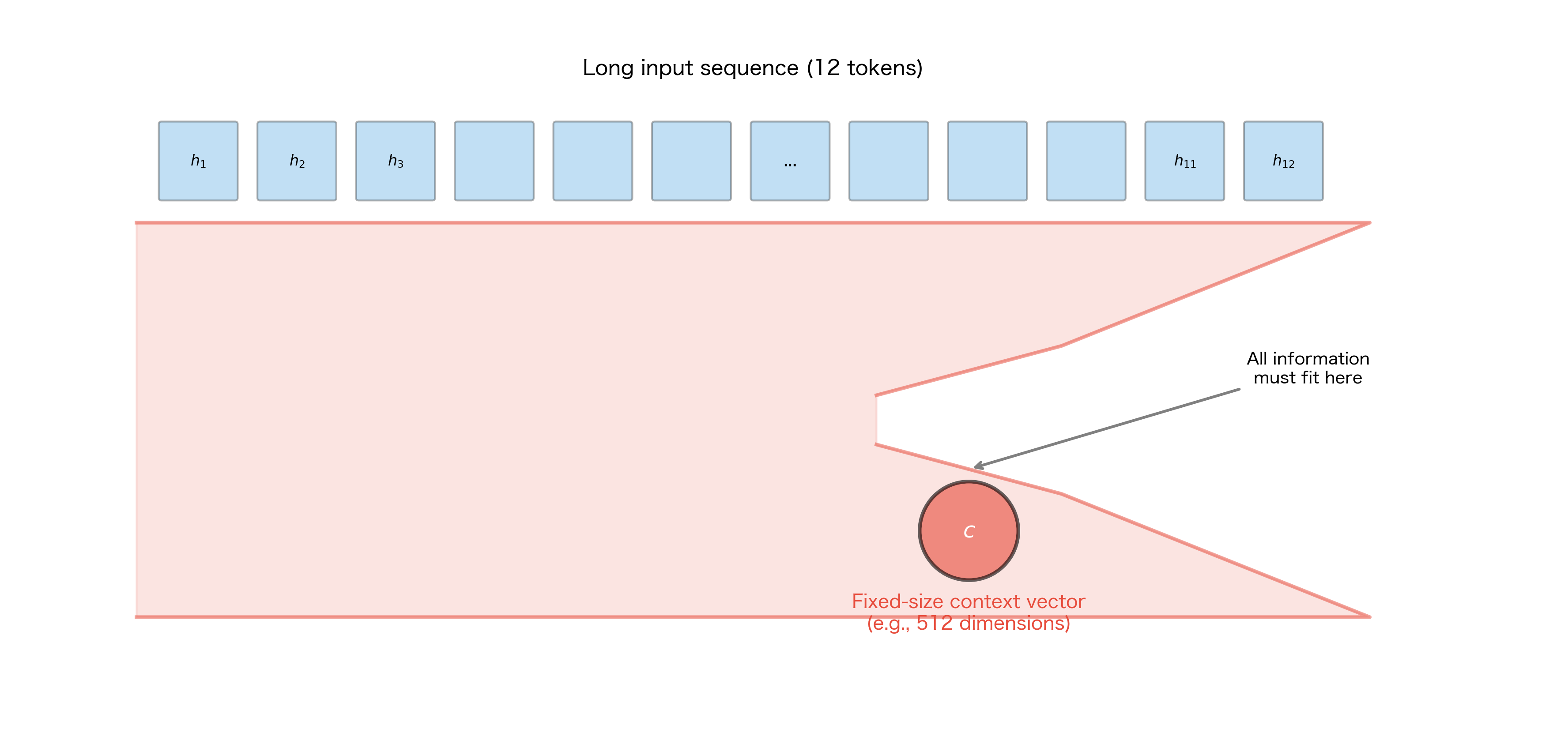
Consider what happens when translating a long sentence. The encoder must compress all the nuances, word relationships, and semantic content into perhaps 512 or 1024 numbers. Early words in the sequence are processed many timesteps before the context vector is formed, so their information must survive through many LSTM updates. Despite the LSTM's gating mechanisms, some information inevitably degrades.
This bottleneck manifests in several ways:
- Translation quality degrades for long sentences: Research showed that basic seq2seq models performed well on sentences under 20 words but quality dropped sharply for longer inputs
- The decoder lacks access to specific source positions: When generating a word, the decoder can't "look back" at a specific part of the input
- Information about word order can be lost: The context vector may capture what concepts are present but lose their precise arrangement
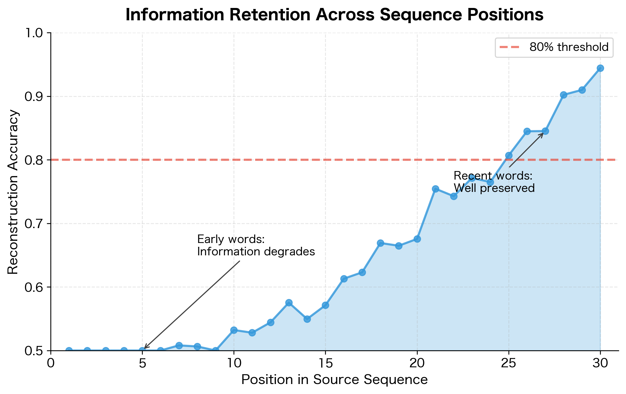
We can visualize this degradation by examining how well the decoder can reconstruct different parts of the input:
The attention mechanism, which we'll cover later in this part, directly addresses the bottleneck problem by allowing the decoder to access all encoder hidden states, not just the final one. But understanding the bottleneck is crucial for appreciating why attention was such an important breakthrough.
The bottleneck's impact on real-world performance was documented in the original seq2seq papers. Translation quality, measured by BLEU score, degrades systematically as source sentences get longer:
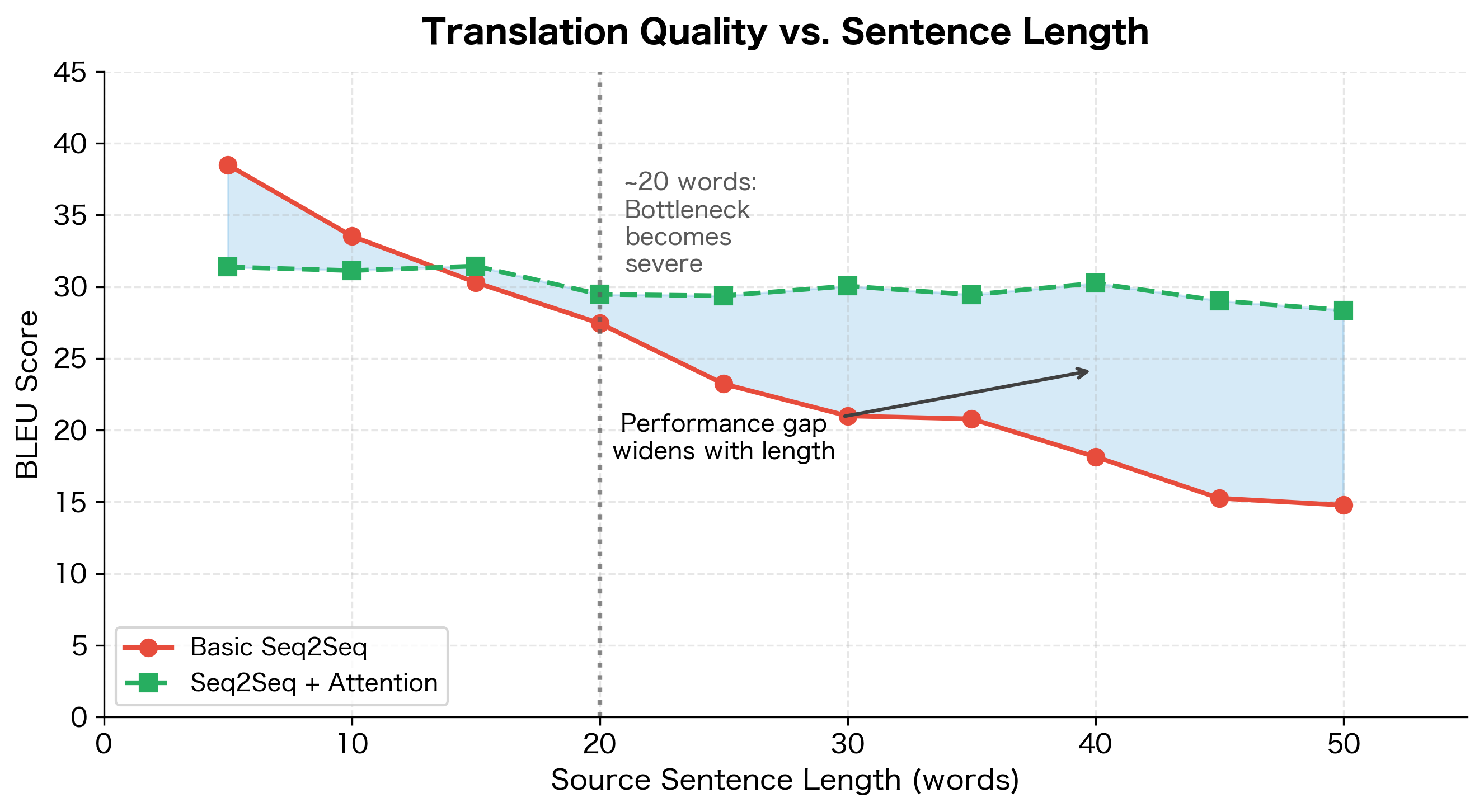
This empirical observation was a key motivation for developing attention. Basic seq2seq models achieve competitive BLEU scores on short sentences (under 20 words) but performance drops sharply for longer inputs. The attention mechanism, shown as the dashed line, maintains quality regardless of length by allowing the decoder to directly access relevant parts of the source sequence rather than relying solely on the compressed context vector.
Seq2Seq for Machine Translation
Machine translation was the driving application for encoder-decoder models. Let's walk through a complete example of how the model processes a translation task.
The Translation Pipeline
Consider translating "The cat sat on the mat" to French. The pipeline proceeds as follows:
- Tokenization: Convert the English sentence to token indices using a source vocabulary
- Encoding: Process tokens through the encoder to get the context vector
- Decoding: Generate French tokens one at a time, starting with a start token
- Detokenization: Convert output indices back to French words
The source sentence maps to indices [3, 4, 5, 6, 3, 7], where repeated words like "the" map to the same index (3). The target includes the start token <s> (index 1) prepended, which tells the decoder to begin generating. Notice that the source has 6 tokens while the target has 8, demonstrating how seq2seq handles variable-length mappings.
Training the Translation Model
During training, we use teacher forcing: the decoder receives the correct previous token at each step, not its own predictions. This allows parallel computation and stable training:
The loss computation deserves attention. We compare the model's predictions (excluding the last position, which predicts beyond the sequence) against the target tokens (excluding the start token, which is input not output). This offset alignment is crucial for correct training.
Inference: Generating Translations
At inference time, we don't have the target sequence. We must generate tokens autoregressively, feeding each prediction back as input for the next step:
This greedy decoding always selects the most probable next token. In practice, beam search (covered in a later chapter) often produces better results by exploring multiple hypotheses simultaneously.
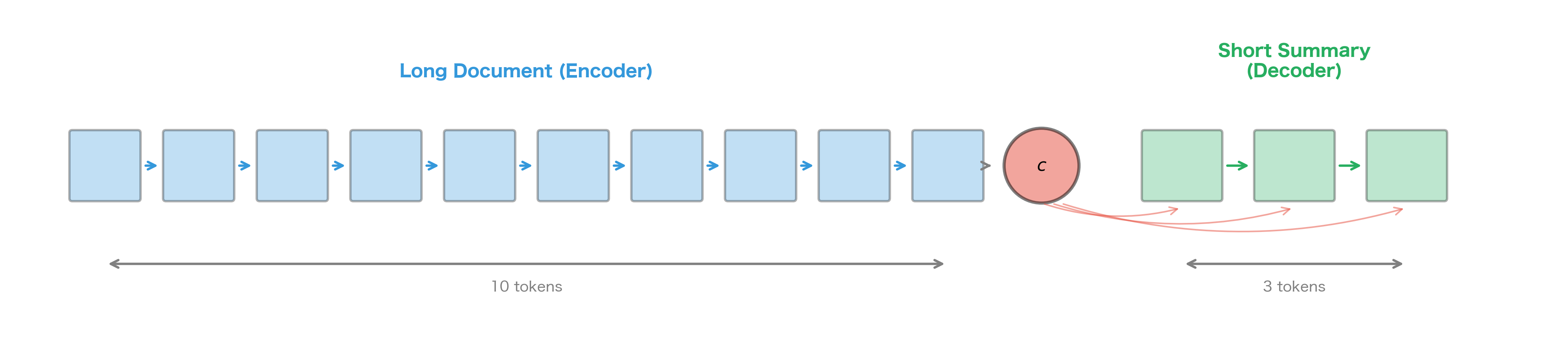
Seq2Seq for Text Summarization
Machine translation maps sequences of similar lengths, but the encoder-decoder framework handles arbitrary length ratios. Text summarization compresses long documents into short summaries, making it another natural application.
Summarization presents unique challenges compared to translation:
- Extreme compression ratios: A 500-word article might become a 50-word summary, requiring 10:1 compression
- Content selection: The model must decide what information is important enough to include
- Abstraction vs extraction: Should the summary use words from the source or generate new phrasings?
The basic encoder-decoder model struggles with these challenges. The bottleneck problem is especially severe when compressing long documents. Later innovations like attention and copy mechanisms significantly improved summarization quality.
Training Setup and Considerations
Training seq2seq models requires careful attention to several practical details: choosing an appropriate loss function, handling variable-length sequences through padding and masking, preventing gradient explosions, and tuning the learning rate schedule. This section covers each of these considerations with practical code examples.
Loss Function
We use cross-entropy loss to train the model. At each position in the output sequence, the model predicts a probability distribution over the vocabulary, and we penalize it based on how much probability it assigns to the correct token. Summing these penalties across all positions gives us the total loss for a sequence:
where:
- : the total loss for the sequence (lower is better)
- : the length of the target sequence
- : the correct (ground truth) target token at position
- : all target tokens before position , i.e.,
- : the context vector from the encoder
- : the probability the model assigns to the correct token , given the context and previous tokens
The negative log transforms probabilities into losses: when the model assigns probability 1.0 to the correct token, (no loss). When it assigns probability 0.01, (high loss). This encourages the model to assign high probability to the correct next token at every position.
Let's visualize this relationship to build intuition for how cross-entropy loss penalizes predictions:
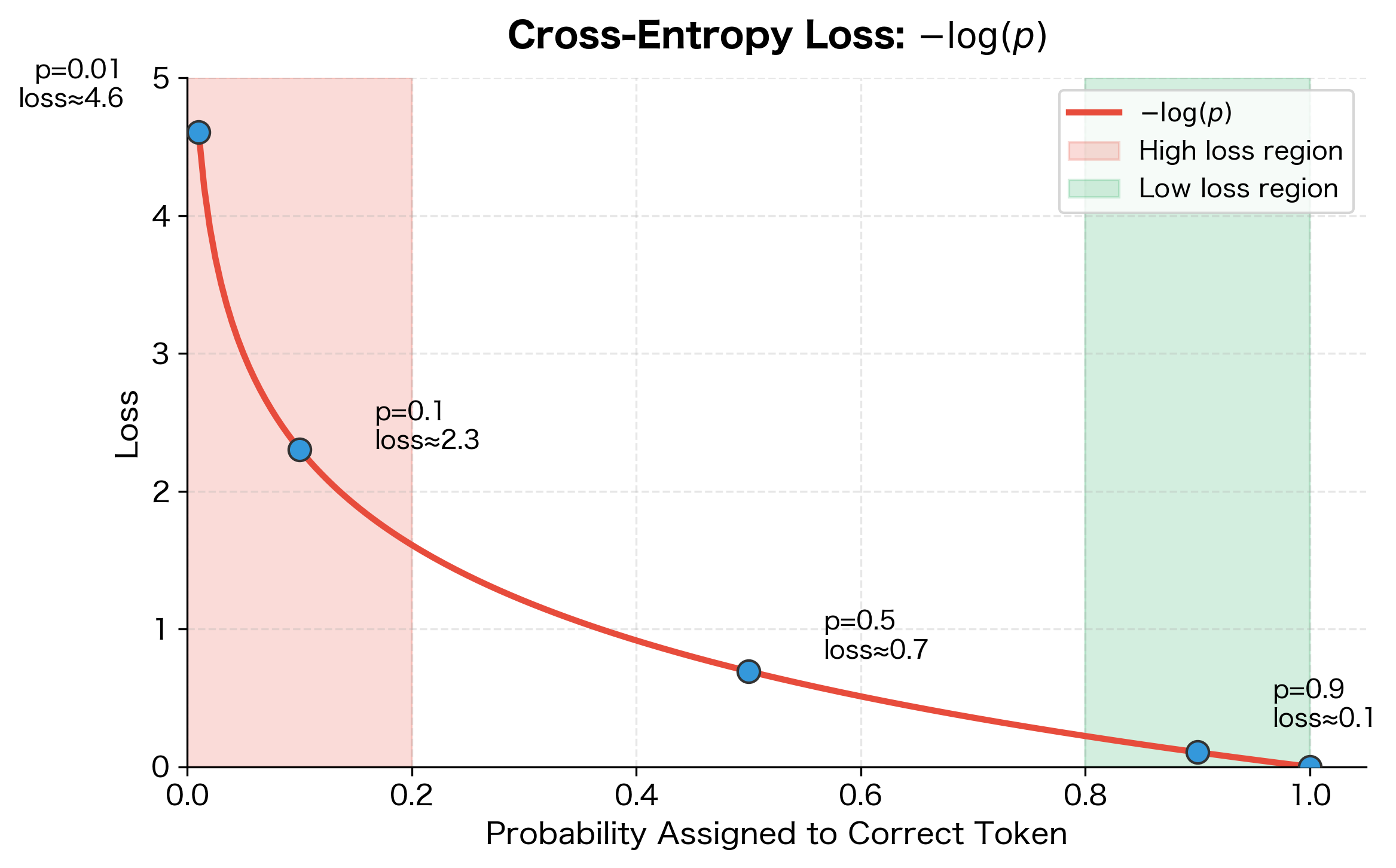
The curve shows why cross-entropy is effective for training: it penalizes confidently wrong predictions much more severely than uncertain ones. A model that assigns only 1% probability to the correct token incurs 20× more loss than one assigning 50%. This steep gradient in the low-probability region provides strong learning signal when the model makes mistakes.
Handling Variable-Length Sequences
Real data contains sequences of varying lengths. We handle this through padding and masking:
The padded tensor shows zeros appended to shorter sequences to match the maximum length of 6. The mask tensor marks which positions contain real tokens (True) versus padding (False). During loss computation, we use this mask to ensure the model isn't penalized for predictions at padded positions, which would distort the training signal.
The mask is used during loss computation to ignore predictions at padded positions. PyTorch's CrossEntropyLoss supports an ignore_index parameter for this purpose.
Gradient Clipping
Seq2seq models are prone to exploding gradients due to the long computational graphs created by unrolling through time. Gradient clipping limits the gradient magnitude:
A typical value is 1.0 or 5.0. Without clipping, training often diverges with NaN losses.
Learning Rate and Optimization
Adam optimizer with learning rate scheduling works well for seq2seq models:
Starting with a learning rate around and reducing it when progress stalls typically works well.
A typical training run shows characteristic loss curves as the model learns to translate:
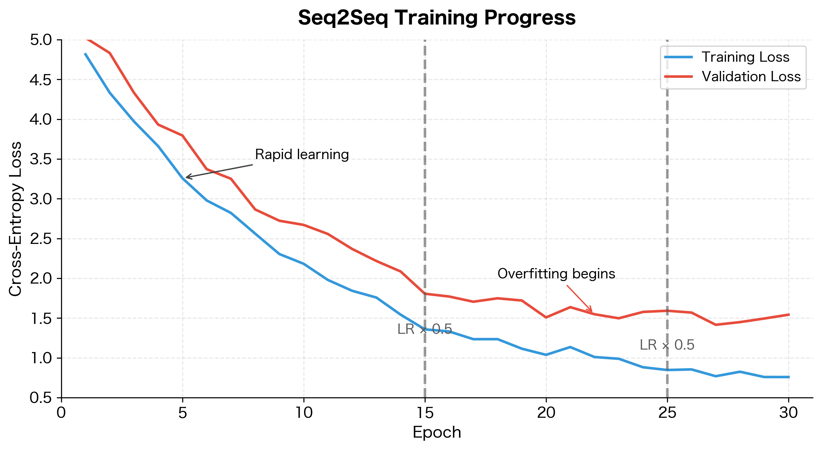
This visualization shows several important training dynamics. Early epochs show rapid loss reduction as the model learns basic translation patterns. The gap between training and validation loss indicates generalization: a small gap means the model generalizes well, while a growing gap signals overfitting. Learning rate reductions (marked by vertical lines) help the model escape local minima and continue improving. The best model checkpoint is typically saved when validation loss is lowest, around epoch 18-20 in this example.
Putting It Together: A Complete Training Loop
Let's implement a complete training loop that incorporates all these considerations:
Limitations and Impact
The encoder-decoder framework was a breakthrough that enabled end-to-end learning for sequence-to-sequence tasks. Before this architecture, machine translation relied on complex pipelines with separate components for alignment, phrase extraction, and language modeling. The seq2seq approach replaced all of this with a single neural network trained end-to-end.
However, the basic architecture has significant limitations that motivated subsequent research. The context vector bottleneck forces all source information through a fixed-size vector, causing information loss for long sequences. Sutskever et al.'s original paper showed that reversing the source sequence improved results, likely because it reduced the average distance between corresponding words in source and target. This hack highlighted the underlying problem: the model struggled to preserve information about early source tokens.
The rigid encoder-decoder separation also limits flexibility. The encoder must finish processing before the decoder can start, preventing any interaction between reading and writing. Human translators don't work this way. They might read part of a sentence, start translating, then look back at the source for clarification. The attention mechanism, which we'll cover in subsequent chapters, addresses this by allowing the decoder to "look back" at any part of the encoded sequence.
Despite these limitations, the encoder-decoder framework established several principles that remain central to modern sequence modeling. The idea of encoding variable-length input into a fixed representation, then decoding back to variable-length output, appears in countless architectures. The separation of understanding (encoding) from generation (decoding) provides a clean abstraction that simplifies model design. And the end-to-end training paradigm, where the entire system is optimized jointly for the final task, has become the dominant approach in NLP.
The seq2seq architecture also demonstrated the power of recurrent networks for complex language tasks. While transformers have since surpassed RNN-based models on most benchmarks, the conceptual framework of encoder-decoder remains. Modern transformer models like T5 and BART use the same high-level architecture: encode the input, then decode the output. The attention mechanism that made transformers possible was first developed to address the bottleneck problem in RNN-based seq2seq models.
Summary
This chapter introduced the encoder-decoder framework, the foundational architecture for sequence-to-sequence learning. We covered how this paradigm separates the tasks of understanding input sequences and generating output sequences, enabling applications like machine translation and text summarization.
The encoder processes the input sequence through an RNN, compressing it into a fixed-size context vector that represents the input's meaning. The decoder, initialized with this context vector, generates the output sequence one token at a time, using each prediction as input for the next step.
The context vector bottleneck is the key limitation of basic seq2seq models. All information about the input must pass through this single vector, causing information loss for long sequences. This bottleneck motivated the development of attention mechanisms, which we'll explore in upcoming chapters.
Key implementation details include:
- Use LSTM or GRU cells for both encoder and decoder to capture long-range dependencies
- Initialize the decoder's hidden state with the encoder's final hidden state
- Apply teacher forcing during training, feeding correct tokens rather than predictions
- Use cross-entropy loss with masking to handle variable-length sequences
- Clip gradients to prevent exploding gradients during backpropagation
The encoder-decoder framework established the paradigm for sequence-to-sequence learning that persists in modern architectures. While attention and transformers have improved upon the basic design, the core insight of separating encoding from decoding remains central to how we approach sequence transformation tasks.
In the next chapter, we'll examine teacher forcing in detail, understanding both its benefits for training efficiency and its drawbacks in terms of exposure bias.
Key Parameters
When building encoder-decoder models with PyTorch's nn.LSTM or nn.GRU, these parameters have the most significant impact on model behavior:
| Parameter | Typical Values | Description |
|---|---|---|
hidden_size | 256-1024 | Dimensionality of the hidden state and context vector. For translation, 512 is a common starting point. The context vector bottleneck makes this choice critical: too small and information is lost, too large and training becomes slow. |
num_layers | 2-4 | Number of stacked RNN layers in both encoder and decoder. Deeper networks capture more complex patterns but require careful initialization and may need residual connections for stable training. |
embed_size | 256-512 | Dimensionality of token embeddings. Should be large enough to capture semantic distinctions but not so large that it dominates parameter count. |
dropout | 0.1-0.3 | Probability of dropping connections between LSTM layers (only active when num_layers > 1). Applied between layers, not within recurrent connections. |
batch_first | True | When True, input tensors have shape (batch, seq_len, features). Using batch_first=True aligns with common data loading patterns and makes debugging easier. |
For training, the following parameters control optimization behavior:
| Parameter | Typical Values | Description |
|---|---|---|
learning_rate | 0.001 | Initial learning rate for Adam optimizer. Reduce on plateau. Too high causes instability, too low causes slow convergence. |
clip_grad | 1.0-5.0 | Maximum gradient norm for clipping. Prevents exploding gradients. Essential for stable training of deep seq2seq models. |
ignore_index | 0 (pad token) | Index to ignore in cross-entropy loss (typically the padding token index). Ensures padded positions don't contribute to the loss. |
Quiz
Ready to test your understanding? Take this quick quiz to reinforce what you've learned about the encoder-decoder framework and sequence-to-sequence models.

Comments