Self-Attention Concept: From Cross-Attention to Contextual Representations

In the previous chapter, we explored attention in encoder-decoder models where the decoder attends to encoder states. This is cross-attention: one sequence attending to a different sequence. But what if a sequence could attend to itself? This simple shift in perspective gives rise to self-attention, the mechanism that powers transformer models and modern language AI.

Self-attention allows each position in a sequence to directly interact with every other position. Instead of processing tokens one at a time through recurrent connections, self-attention computes relationships between all pairs of tokens simultaneously. This architectural change enables parallelization during training and captures long-range dependencies without the vanishing gradient problems that plague RNNs.

In encoder-decoder attention, we have two distinct sequences: the encoder outputs serve as keys and values, while the decoder state provides the query. The decoder asks, "Which parts of the input are relevant to what I'm generating right now?"

Self-attention simplifies this setup. Instead of attending across two different sequences, a single sequence attends to itself. Every token in the sequence serves simultaneously as a query, a key, and a value. The question becomes: "For each token in this sequence, which other tokens are most relevant to understanding its meaning in context?"

Consider the sentence "The animal didn't cross the street because it was too tired." To understand what "it" refers to, you need to connect it back to "animal" rather than "street." Self-attention enables this by allowing "it" to attend strongly to "animal," building a representation that captures this coreference relationship.

The key insight is that the meaning of a word depends heavily on its context. The word "bank" means something different in "river bank" versus "bank account." Self-attention lets each word gather information from surrounding words to disambiguate and enrich its representation.

The defining characteristic of self-attention is all-pairs interaction. For a sequence of $n$ tokens, self-attention computes interactions between all $n^2$ pairs of positions. Why $n^2$? Each of the $n$ tokens must compute its relationship with every other token, including itself. Token 1 interacts with tokens 1 through $n$ (that's $n$ interactions), token 2 does the same (another $n$ interactions), and so on for all $n$ tokens, giving us $n \times n = n^2$ total interactions.

This is fundamentally different from recurrent models, which process tokens sequentially and must pass information through intermediate states.

In an RNN, if you want information from position 1 to reach position 100, it must flow through 99 intermediate hidden states. Each step risks losing or distorting information. Self-attention eliminates this problem by computing direct connections between any two positions.

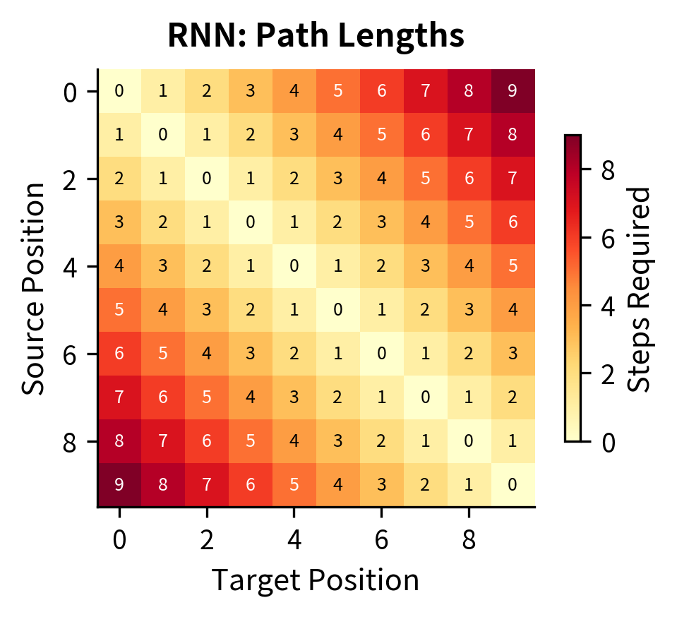
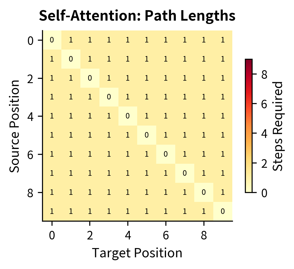
The contrast is striking. In the RNN heatmap (left), path lengths grow with distance: connecting position 0 to position 9 requires 9 steps, shown by the dark red corners. The self-attention heatmap (right) is nearly uniform: every position connects to every other position in exactly 1 step (with 0 for self-connections on the diagonal). This constant path length is crucial for capturing long-range dependencies without information degradation.

Self-attention excels at building contextual representations. A word embedding from Word2Vec or GloVe assigns the same vector to "bank" regardless of context. Self-attention creates contextualized embeddings where each token's representation incorporates information from surrounding tokens.

The process works as follows. Each token starts with an initial embedding. Through self-attention, each token gathers information from all other tokens, weighted by relevance. The output is a new set of representations where each token "knows about" the full sequence context.

This contextual awareness enables several capabilities that static embeddings lack:

• Word sense disambiguation: The representation of "bank" differs based on surrounding words
• Coreference resolution: Pronouns can gather information from their antecedents
• Syntactic awareness: Verbs can connect to their subjects and objects regardless of distance
• Semantic composition: Phrases and sentences build meaning from their constituent words

Let's visualize how self-attention might weight different tokens when processing a simple sentence.

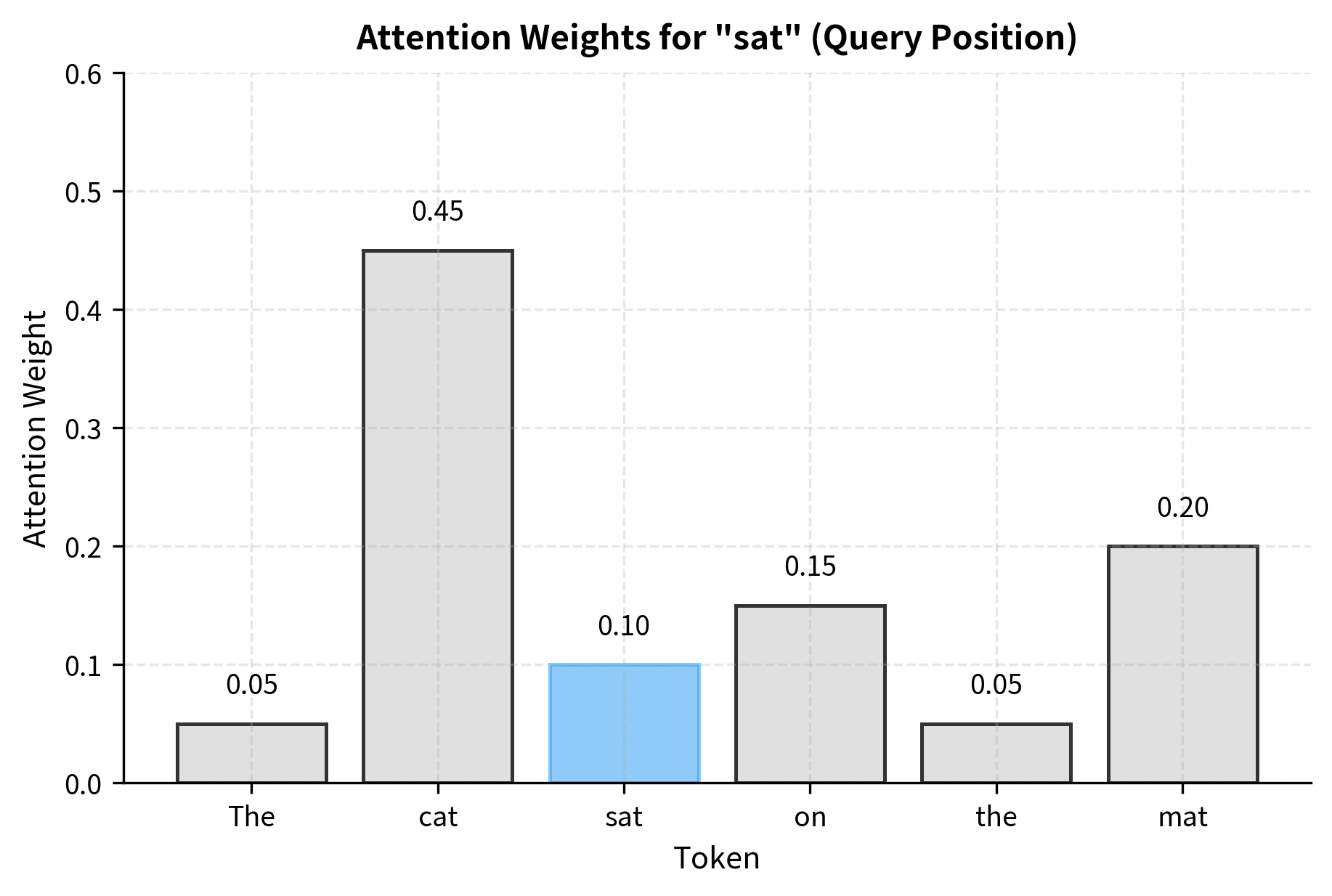
The visualization shows that when building a representation for "sat," the model attends most strongly to "cat" (the subject performing the action) and "mat" (the location). Function words like "the" and "on" receive less attention. This weighted combination creates a rich representation that captures the verb's relationship to other sentence elements.

Now that we understand why self-attention is useful, let's examine how it actually works. The core idea is elegantly simple: to build a contextual representation for any token, we take a weighted average of all tokens in the sequence. The weights reflect how relevant each token is to the one we're updating.

Think of it like asking every word in a sentence: "How much should I pay attention to you when trying to understand myself?" Words that are more relevant get higher weights, and their information contributes more to the final representation.

Self-attention follows a consistent three-stage pattern:

1. Compute similarity scores: For each pair of positions, calculate a number indicating how relevant one is to the other. High scores mean strong relevance.

2. Normalize to weights: Raw scores can be any real number. We need to convert them into proper weights that sum to 1, so we can interpret them as "how much attention to pay." The softmax function handles this conversion.

3. Aggregate values: Finally, compute a weighted sum of all positions' representations. Positions with higher weights contribute more to the output.

This pipeline runs for every position simultaneously, producing a new set of contextual embeddings where each token has gathered information from the entire sequence.

Let's formalize this intuition. Suppose we have a sequence of $n$ tokens, each represented by a $d$-dimensional embedding vector. We can write the input as a matrix:

where each $\mathbf{x}_i \in \mathbb{R}^d$ is the embedding for token $i$.

Stage 1: Similarity Scores

How do we measure relevance between two tokens? The simplest approach uses the dot product. If two embedding vectors point in similar directions, their dot product is large and positive. If they're orthogonal (unrelated), the dot product is zero. This gives us a natural measure of similarity.

For positions $i$ and $j$, the similarity score is:

where:

• $s_{ij}$: the raw similarity score between positions $i$ and $j$
• $\mathbf{x}_i \cdot \mathbf{x}_j$: the dot product of the two embedding vectors
• $d$: the embedding dimension

The dot product captures semantic similarity: tokens with similar meanings tend to have similar embeddings, producing high dot products.

Stage 2: Softmax Normalization

Raw dot products can be any real number, positive or negative, with no upper bound. To use them as weights for averaging, we need to transform them into a probability distribution. The softmax function accomplishes this:

where:

• $\alpha_{ij}$: the attention weight from position $i$ to position $j$
• $\exp(s_{ij})$: the exponential function applied to the similarity score, ensuring positivity
• $\sum_{k=1}^{n} \exp(s_{ik})$: the normalizing constant that makes all weights from position $i$ sum to 1

Why softmax? It has two crucial properties:

1. Positivity: The exponential function maps any real number to a positive value, so all weights are positive.
2. Normalization: Dividing by the sum ensures $\sum_{j=1}^{n} \alpha_{ij} = 1$, giving us valid weights for a weighted average.

Additionally, softmax amplifies differences: if one score is much higher than others, its weight dominates. This allows the model to focus sharply on the most relevant tokens when appropriate.

Stage 3: Weighted Aggregation

With attention weights in hand, we compute the output representation for each position as a weighted sum of all input embeddings:

where:

• $\mathbf{y}_i$: the output representation for position $i$, now enriched with contextual information
• $\alpha_{ij}$: the attention weight determining how much position $j$ contributes to position $i$'s output
• $\mathbf{x}_j$: the input embedding at position $j$

This formula is the heart of self-attention. Each output $\mathbf{y}_i$ is a blend of all inputs, with the blending proportions determined by the learned attention weights. Tokens that are highly relevant to position $i$ contribute strongly; irrelevant tokens contribute little.

The complete self-attention computation flows naturally from these three stages. For every position $i$ in the sequence:

1. Compute dot products with all positions: $s_{ij} = \mathbf{x}_i \cdot \mathbf{x}_j$ for $j = 1, \ldots, n$
2. Apply softmax to get attention weights: $\alpha_{ij} = \text{softmax}(s_{i1}, s_{i2}, \ldots, s_{in})_j$
3. Compute weighted sum: $\mathbf{y}_i = \sum_{j=1}^{n} \alpha_{ij} \mathbf{x}_j$

Because each position's computation is independent of the others, we can process all $n$ positions in parallel. This parallelism is what makes self-attention so efficient on modern GPU hardware.

Let's translate this mathematical framework into code. We'll implement a simple self-attention function that takes a sequence of embeddings and returns the contextual outputs along with the attention weights.

Notice how the implementation mirrors the three-stage formula. The matrix multiplication embeddings @ embeddings.T computes all $n^2$ dot products simultaneously: entry $(i, j)$ contains $\mathbf{x}_i \cdot \mathbf{x}_j$. The softmax is applied row-wise, so each row of attention weights sums to 1. Finally, multiplying the attention weights by the embeddings computes all weighted sums in parallel.

Let's test this on a small sequence to see the attention mechanism in action:

The attention weight matrix is $n \times n$, where entry $(i, j)$ tells us how much position $i$ attends to position $j$. Each row sums to exactly 1.0, confirming that softmax produces valid probability distributions. The output has the same shape as the input: each of our 4 tokens now has a new 8-dimensional representation that incorporates information from all other tokens.

A heatmap provides an intuitive view of self-attention patterns. Rows represent query positions (which token is gathering information), and columns represent key positions (which tokens are being attended to). Darker cells indicate stronger attention.

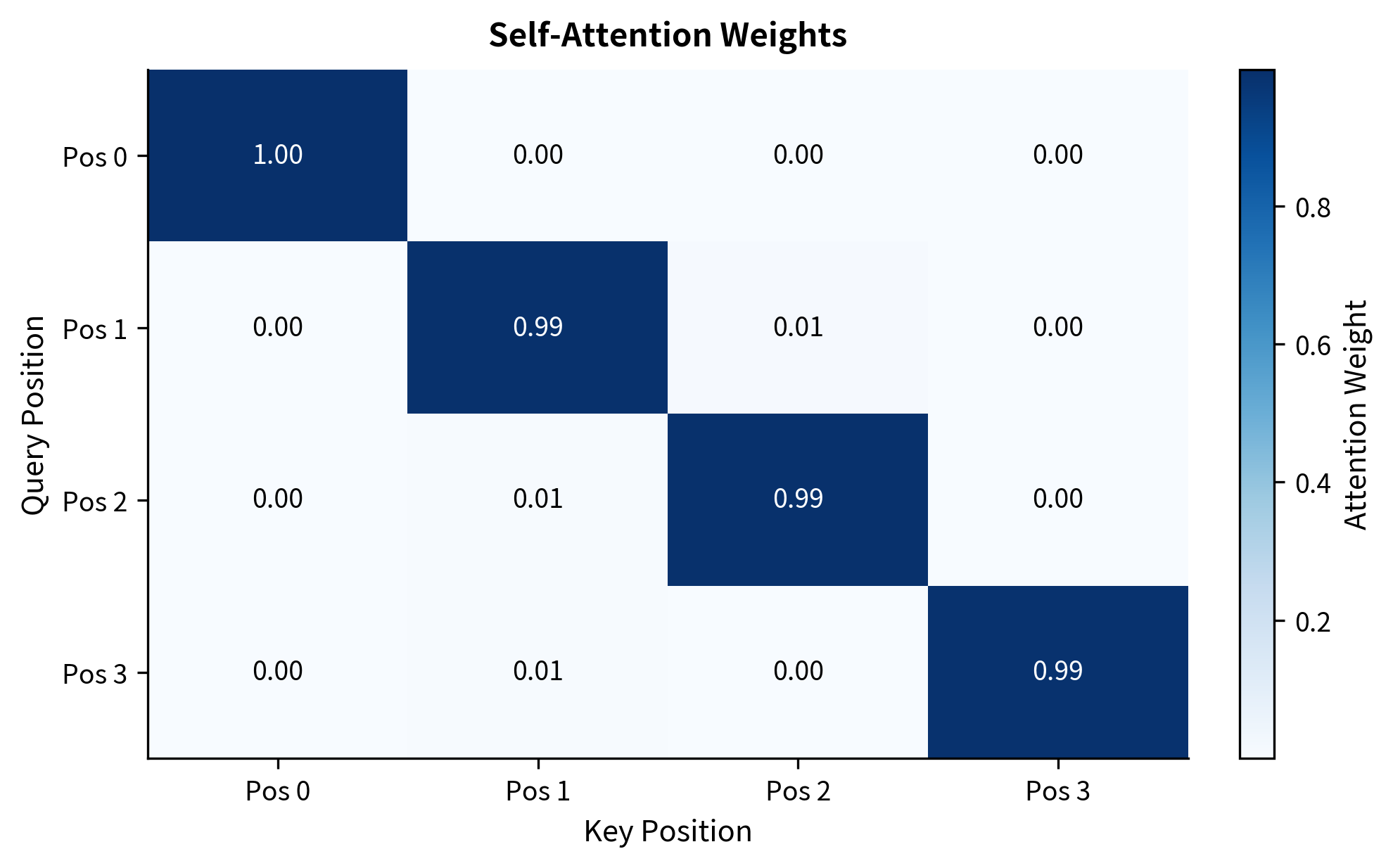
In this random example, we see some diagonal emphasis where tokens attend to themselves, plus distributed attention to other positions. In trained models, these patterns become meaningful: related words attend strongly to each other, syntactic structures emerge, and semantic relationships become visible.

Self-attention and recurrence represent fundamentally different approaches to sequence modeling. Understanding their trade-offs clarifies why transformers have largely replaced RNNs for most NLP tasks.

Parallelization: RNNs process tokens sequentially because each hidden state depends on the previous one. Self-attention computes all pairwise interactions simultaneously, enabling massive parallelization on GPUs. This difference dramatically accelerates training on modern hardware.

Long-range dependencies: In an RNN, information must flow through many timesteps to connect distant positions. Gradients can vanish or explode along this path. Self-attention connects any two positions directly, making it easier to learn long-range dependencies.

Computational complexity: Self-attention computes $n^2$ pairwise interactions for a sequence of length $n$, where $n$ is the number of tokens. RNNs have linear complexity, meaning their computational cost grows proportionally to $n$. For very long sequences, the quadratic cost of self-attention becomes prohibitive: doubling the sequence length quadruples the computation. This motivates efficient attention variants.

Positional information: RNNs inherently encode position through their sequential processing. Self-attention treats all positions symmetrically and requires explicit positional encodings to distinguish word order. We'll cover positional encodings in a later chapter.

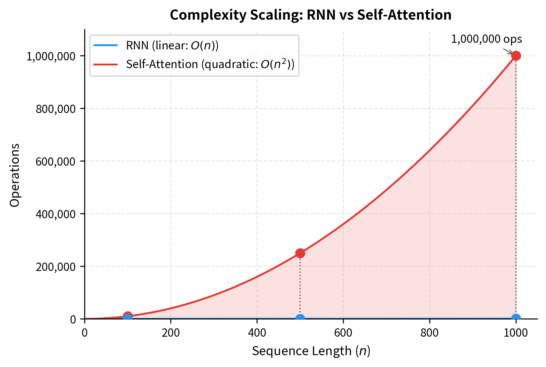
The quadratic growth of self-attention is dramatic: at sequence length 1000, self-attention requires 1 million operations compared to just 1000 for an RNN. However, self-attention's operations are independent and can run in parallel on GPUs, while RNN operations must be sequential. This trade-off explains why transformers dominate despite higher theoretical complexity: parallelism wins on modern hardware.

The formulas become clearer when we trace through a concrete example step by step. Let's process a three-word sequence, "I love coffee," using tiny 2-dimensional embeddings. With only 2 dimensions, we can easily verify each calculation by hand and visualize what's happening geometrically.

We'll assign each word an embedding that points in a different direction:

These embeddings form a simple geometric arrangement: "I" points east, "coffee" points north, and "love" points northeast, lying exactly between them. This setup will help us understand how the dot product captures similarity.

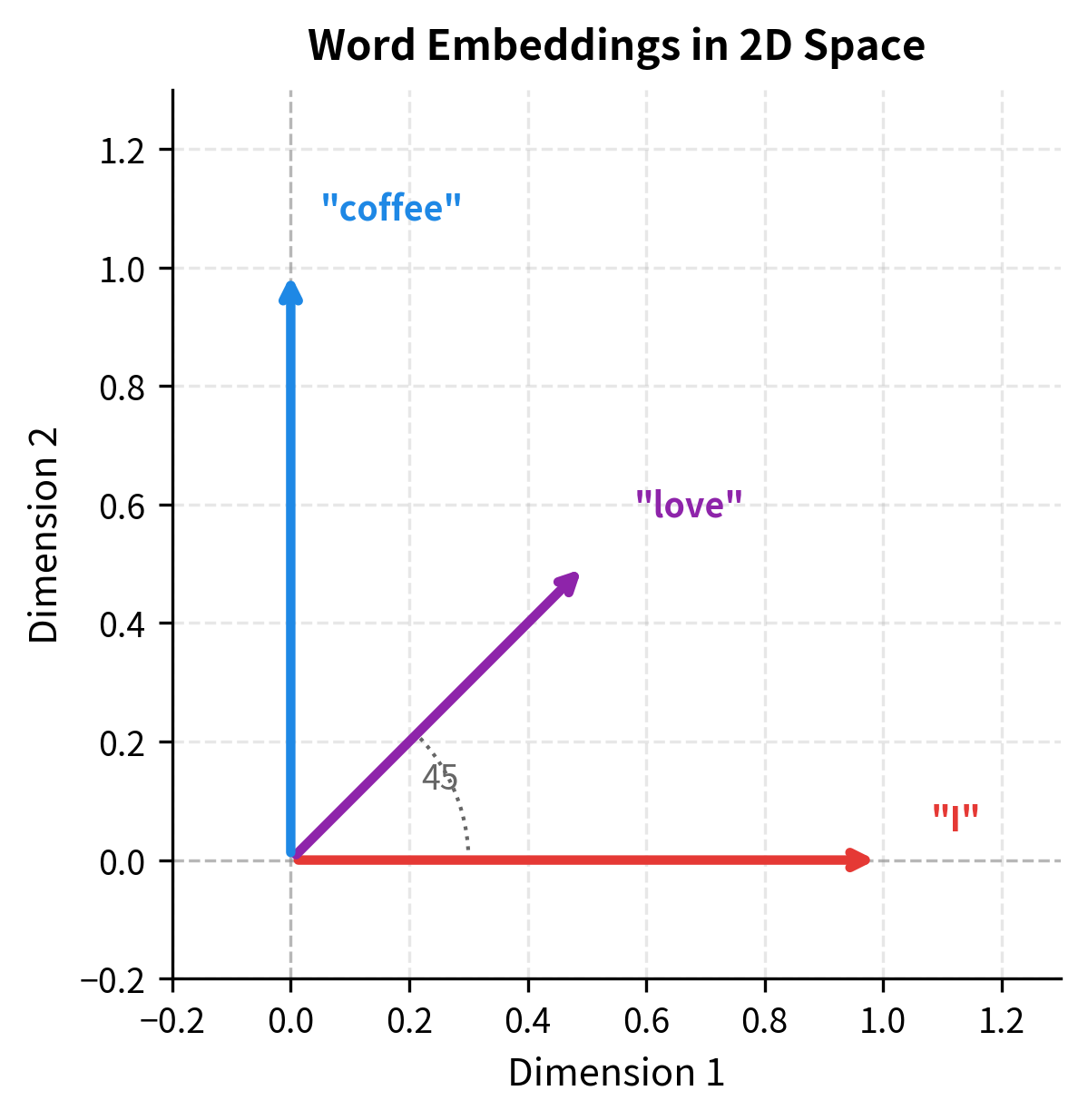
The geometric arrangement makes the dot product intuition clear: vectors pointing in similar directions have high dot products, while perpendicular vectors have zero dot product.

First, we compute the dot product between every pair of words. Remember, the dot product $\mathbf{x}_i \cdot \mathbf{x}_j$ measures how much two vectors point in the same direction.

Let's interpret this matrix:

• Diagonal entries (1.00, 0.50, 1.00): These are self-similarities. "I" and "coffee" have unit-length embeddings, so their self-dot-products are 1.0. "love" has length $\sqrt{0.5^2 + 0.5^2} = \sqrt{0.5} \approx 0.71$, giving a self-dot-product of 0.5.

• "I" vs "coffee" (0.00): These vectors are perpendicular (orthogonal), so their dot product is zero. In embedding space, this means they're unrelated.

• "love" vs others (0.50): "love" points between "I" and "coffee," giving it moderate similarity to both. The dot product of 0.5 reflects this intermediate relationship.

Raw dot products aren't suitable weights for averaging because they don't sum to 1. The softmax function transforms each row into a probability distribution:

Now each row sums to 1.0, and we can interpret the values as "attention percentages":

• "I" attends most to itself (about 58%), moderately to "love" (31%), and least to "coffee" (11%). This makes sense: "I" had the highest dot product with itself, moderate with "love," and zero with "coffee."

• "love" distributes attention more evenly across all three words (about 33% each). Its embedding lies between the others, giving it similar dot products with everyone.

• "coffee" mirrors "I": it attends mostly to itself, moderately to "love," and barely to "I."

The softmax has transformed our raw similarities into a meaningful attention distribution. Higher similarity scores become higher attention weights, but even zero-similarity pairs get some weight (the exponential of 0 is 1, not 0).

Finally, we use these attention weights to compute a weighted average of all embeddings for each position:

The transformation is subtle but meaningful. Each word's representation has shifted toward the other words, with the amount of shift determined by the attention weights:

• "I" started at [1.0, 0.0] and moved to approximately [0.73, 0.27]. It picked up some "northward" component from "love" and "coffee."

• "love" started at [0.5, 0.5] and stayed close to its original position. Because it attended fairly evenly to all words, and it was already in the "middle," the weighted average didn't change it much.

• "coffee" started at [0.0, 1.0] and moved to approximately [0.27, 0.73]. It picked up some "eastward" component from "I" and "love."

This is the essence of self-attention: each word's output is no longer just its own embedding, but a blend of all words' embeddings, weighted by relevance. The word "I" now "knows about" the context of "love" and "coffee." This contextual blending is what enables transformers to build rich, context-dependent representations.

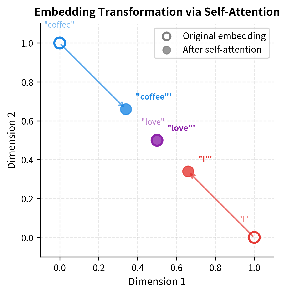
The visualization captures the essence of self-attention geometrically. Each word's representation moves toward the center of mass of all words, weighted by attention. "I" and "coffee" shift significantly toward each other (via "love"), while "love" barely moves because it was already centrally positioned. After this transformation, all three words carry information about the full context.

Self-attention transformed NLP by enabling parallel processing and direct long-range connections. The transformer architecture, built on self-attention, powers models like BERT, GPT, and their successors. These models achieve state-of-the-art results across virtually all NLP benchmarks.

However, self-attention has significant limitations. The quadratic complexity in sequence length makes it expensive for long documents. Processing a 10,000-token document requires computing 100 million pairwise interactions. This has motivated research into efficient attention variants like Longformer, BigBird, and linear attention mechanisms that reduce complexity while preserving much of self-attention's power.

Self-attention also lacks inherent positional awareness. Unlike RNNs, which process tokens in order, self-attention treats the sequence as a set. The sentence "dog bites man" would produce the same attention weights as "man bites dog" without explicit positional information. Transformers address this with positional encodings, but the need for this additional component reveals a fundamental limitation of the attention mechanism itself.

Despite these challenges, self-attention's benefits outweigh its costs for most NLP applications. The ability to train on massive datasets with full parallelization, combined with the capacity to model arbitrary dependencies, has made transformer-based models the dominant paradigm in modern language AI.

Self-attention is the mechanism that allows a sequence to attend to itself, enabling each position to gather information from all other positions. This simple idea has profound implications for how we build language models.

Key takeaways from this chapter:

• Self-attention vs cross-attention: In cross-attention, one sequence attends to another. In self-attention, a sequence attends to itself, with each token serving as query, key, and value.
• All-pairs interaction: Self-attention computes direct connections between all $n^2$ pairs of positions (where $n$ is the sequence length), eliminating the need for information to flow through intermediate states.
• Contextual representations: By aggregating information from surrounding tokens, self-attention creates embeddings that capture word meaning in context.
• Parallelization: Unlike recurrent models, self-attention computes all interactions simultaneously, enabling efficient training on modern hardware.
• Quadratic complexity: The all-pairs computation scales as $O(n^2)$, meaning computational cost grows with the square of sequence length $n$. This makes self-attention expensive for very long sequences.
• Position agnostic: Self-attention treats sequences as sets, requiring explicit positional encodings to capture word order.

In the next chapter, we'll dive into the mechanics of how self-attention actually computes these interactions. The query, key, and value projections transform input embeddings into specialized representations that enable the attention computation. Understanding these projections is essential for implementing and reasoning about transformer models.

Ready to test your understanding? Take this quick quiz to reinforce what you've learned about self-attention.