

Master CRFs for sequence labeling, from log-linear models to feature functions and the forward algorithm. Learn how CRFs overcome HMM limitations for NER and POS tagging.

This article is part of the free-to-read Language AI Handbook
Choose your expertise level to adjust how many terms are explained. Beginners see more tooltips, experts see fewer to maintain reading flow. Hover over underlined terms for instant definitions.
Conditional Random Fields
Hidden Markov Models brought probabilistic reasoning to sequence labeling, but their generative formulation imposes strong constraints. Each observation depends only on its corresponding hidden state, forcing independence assumptions that conflict with the overlapping, correlated features that make natural language rich and complex. When you see the word "bank," its context matters enormously: preceding words, suffixes, capitalization patterns, surrounding punctuation. HMMs struggle to incorporate such features without violating their independence assumptions.
Conditional Random Fields (CRFs) emerged as a direct response to these limitations. By modeling the conditional probability of labels given observations rather than their joint distribution, CRFs can incorporate arbitrary overlapping features without worrying about dependencies between them. This discriminative approach has become the foundation of modern sequence labeling, powering named entity recognition, POS tagging, and countless other NLP tasks.
This chapter develops CRFs from first principles. We'll examine why HMMs fall short, derive the CRF formulation mathematically, implement feature functions, and build working CRF taggers. By the end, you'll understand not just how to use CRFs but why they work so well for sequence labeling.
From Generative to Discriminative Models
Before diving into CRFs, let's understand the fundamental distinction between generative and discriminative approaches to classification. This distinction explains why CRFs exist and what problems they solve.
Generative models learn the joint probability of inputs and outputs, then use Bayes' rule to compute for prediction. Discriminative models directly learn the conditional probability without modeling the input distribution.
The HMM Approach
Hidden Markov Models are generative. They model how sequences are produced: first, a hidden state is generated according to transition probabilities, then an observation is emitted according to emission probabilities. For a sequence of observations and labels , an HMM models the joint probability of observations and labels:
where:
- : the sequence of observations (e.g., words in a sentence)
- : the sequence of labels (e.g., POS tags or entity types)
- : the initial state probability (probability of starting with label )
- : the transition probability from label to label
- : the emission probability of observing given label
The first product captures transition probabilities (how states follow each other), and the second captures emission probabilities (how each state generates its observation). To predict labels for new observations, we apply Bayes' rule:
where:
- : the posterior probability of label sequence given observations
- : the joint probability computed by the HMM formula above
- : the marginal probability of the observations, obtained by summing over all possible label sequences
This generative formulation imposes a critical constraint: the observation can only depend on its own label , not on other observations or labels. This independence assumption enables tractable inference but limits expressiveness.
The Independence Problem
Consider tagging the word "bank" in context. A good tagger should consider:
- The word itself: "bank"
- The previous word: "river" suggests location, "investment" suggests organization
- The next word: "account" suggests financial meaning
- Capitalization: "Bank" at sentence start vs. "bank" mid-sentence
- Word suffixes: "-ing," "-tion," "-ly" carry grammatical information
- Surrounding punctuation: quotation marks might indicate names
These features overlap and interact. The suffix "-ing" combined with a preceding auxiliary verb strongly suggests a verb tag. Capitalization plus a preceding determiner suggests a proper noun. HMMs cannot naturally express such feature combinations because each observation must be generated independently from its label alone.
In an HMM, we could only condition on the previous tag, not the previous word. The rich contextual features visible in the data cannot be exploited directly.
The Discriminative Solution
CRFs take a fundamentally different approach. Instead of modeling how observations are generated, they directly model the probability of a label sequence given the observations:
This conditional formulation has a crucial advantage: since we condition on , we don't need to model the distribution of observations. Features of can overlap arbitrarily, interact in complex ways, and depend on any part of the input sequence. The model only needs to learn which label sequences are likely given the observed features.
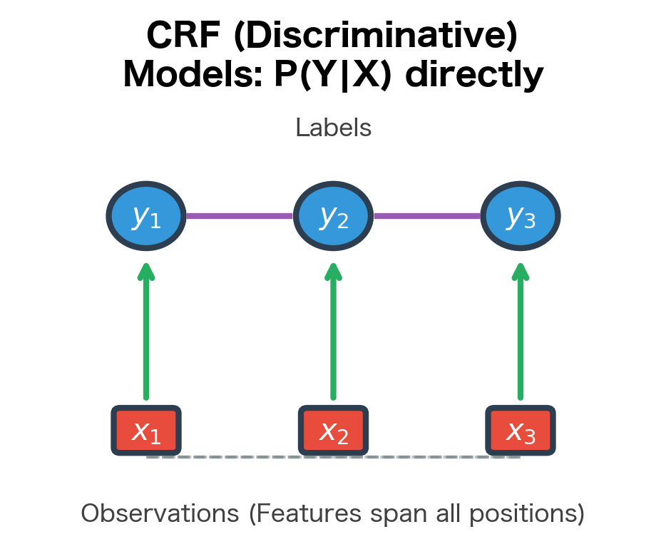
The figure illustrates the fundamental difference. In HMMs, arrows point from hidden states to observations, reflecting the generative process. In CRFs, observations condition the labels, and features can connect any observation to any label. This reversal of direction is not merely notational; it fundamentally changes what the model can represent.
The CRF Formulation
We've established that HMMs struggle with overlapping features because their generative structure demands independence between observations. Now we need a mathematical framework that preserves the sequential structure of HMMs while escaping their independence constraints. The solution lies in a family of models called log-linear models, which CRFs extend to sequences.
This section builds the CRF formulation step by step. We'll start with log-linear models for single classification decisions, then extend them to sequences, and finally examine the feature functions that give CRFs their expressive power. By the end, you'll see how CRFs elegantly solve the problems we identified with HMMs.
Log-Linear Models for Classification
Before tackling sequences, let's understand how log-linear models work for a single classification decision. The core idea is beautifully simple: instead of modeling how observations are generated, we directly score how well each possible label fits the observed input.
Consider classifying a single word. We want to compute , the probability of label given input features . A log-linear model builds this probability in three steps:
- Extract features: Define functions that measure relevant properties of the input-label pair
- Compute a score: Sum the weighted features to get an overall "compatibility score" for each label
- Normalize to probabilities: Convert scores to probabilities using the exponential function and normalization
This yields the fundamental log-linear equation:
Let's unpack each component:
- : the -th feature function, which extracts a property of the input-output pair. These are the building blocks of the model, returning real numbers (often 0 or 1 for binary features).
- : the weight for feature , learned from training data. Positive weights encourage labels where the feature fires; negative weights discourage them.
- : the total score for assigning label to input . This is just a weighted sum of features.
- : the exponential function transforms scores into positive values, ensuring we can interpret results as probabilities.
- : the partition function, which sums over all possible labels to normalize the distribution.
The exponential function serves two purposes. First, it maps any real-valued score to a positive number, which is necessary for probabilities. Second, it has a useful property: if one label's score is much higher than others, the exponential amplifies this difference, making the model confident. If scores are similar, probabilities are more uniform. This "soft-max" behavior emerges naturally from the exponential.
The partition function deserves special attention. It ensures that probabilities sum to 1 by computing the total "mass" across all possible labels. For single classification with a small label set, computing is trivial. But as we'll see, computing for sequences becomes the central computational challenge of CRFs.
Why is this formulation powerful? Because feature functions can capture any aspect of the input-output relationship. Unlike HMMs, where each observation depends only on its label, log-linear models can incorporate overlapping, interacting features without any independence assumptions.
| Label | Raw Score | exp(Score) | Probability |
|---|---|---|---|
| NOUN | 2.0 | 7.4 | 0.001 |
| VERB | 6.5 | 665.1 | 0.996 |
| ADJ | 4.0 | 54.6 | 0.004 |
Notice what happened here. Three features fired for the word "running": the word itself, its suffix, and the preceding word. Each feature contributed to the scores for different labels, and the model combined them through weighted summation. The suffix -ing combined with prev_word=is provides strong evidence for VERB, and the learned weights reflect this intuition. The model assigned VERB a probability of over 99% by combining multiple overlapping features, something an HMM could never do.
Extending to Sequences: Linear-Chain CRFs
The log-linear model handles single classification decisions elegantly. But sequence labeling requires something more: we need to model entire sequences of labels, where each label might depend on its neighbors. How do we extend the log-linear framework to sequences while preserving its ability to use arbitrary features?
The answer is the linear-chain CRF. The key insight is to treat the entire label sequence as a single structured output, then score it using features that can look at adjacent labels and any part of the input. Instead of independently classifying each position, we score complete label sequences and find the one with the highest probability.
For a sequence of observations and labels , the linear-chain CRF defines:
This formula looks similar to the single-classification case, but with a crucial difference: we now sum over positions in the sequence, and feature functions examine pairs of adjacent labels. Let's break it down:
- : We accumulate scores across all positions in the sequence
- : Each feature function now takes four arguments
The four arguments to feature functions are the heart of CRF expressiveness:
| Argument | What it provides | Example use |
|---|---|---|
| Previous label | Capture transition patterns (DET → NOUN) | |
| Current label | Capture emission patterns (word → label) | |
| Entire input sequence | Look at any word, not just current position | |
| Current position | Position-specific features (first word often capitalized) |
This design is deliberate. By including both and , features can model label-label dependencies like HMM transitions. By including the entire sequence rather than just , features can examine context: the previous word, the next word, or even words further away. The position enables features that behave differently at sequence boundaries.
The term "linear-chain" refers to the dependency structure: each label directly depends only on its immediate neighbor . This isn't a limitation of CRFs in general, just a practical choice that enables efficient inference. Higher-order CRFs exist but are exponentially more expensive.
The partition function for sequences presents a computational challenge:
This sum ranges over all possible label sequences . With labels and sequence length , there are possible sequences. For a modest vocabulary of 10 labels and a 20-word sentence, that's sequences, far too many to enumerate. Fortunately, the linear-chain structure enables efficient computation through dynamic programming, which we'll explore in the next section.
Feature Functions in Detail
We've seen that CRFs score sequences using weighted sums of feature functions. But what exactly are these features, and how do we design them? This is where CRFs truly shine: feature functions can capture virtually any pattern you can imagine, from simple word-label associations to complex contextual dependencies.
A feature function maps a (previous label, current label, observation sequence, position) tuple to a real value. Binary features return 1 when a pattern is present and 0 otherwise. The weight determines how much this pattern influences predictions.
Feature functions fall into two main categories, each serving a distinct purpose in the model.
State Features: Linking Observations to Labels
State features capture the relationship between observations and labels. They answer the question: "Given what I observe at this position, which label is most appropriate?"
Consider a feature that fires when the word "bank" appears with the label NOUN:
The notation denotes the indicator function, which returns 1 if the condition is true and 0 otherwise. The product of two indicators returns 1 only when both conditions hold. So this feature "fires" (returns 1) precisely when:
- The current word is "bank", AND
- The current label is NOUN
If the learned weight is positive, this feature increases the score for labeling "bank" as NOUN. If negative, it discourages that labeling. The training process learns these weights from data.
But state features aren't limited to the current word. Because feature functions receive the entire observation sequence , they can examine context:
- Previous word: Does "river" precede this word? (suggests location)
- Next word: Does "account" follow? (suggests financial meaning)
- Suffixes: Does the word end in "-ing"? (suggests verb)
- Capitalization: Is the word capitalized mid-sentence? (suggests proper noun)
This flexibility is what HMMs lack. In an HMM, the observation "bank" can only depend on its own label. In a CRF, the feature for "bank" can simultaneously consider the previous word, the next word, and any other contextual signal.
Transition Features: Modeling Label Dependencies
Transition features capture patterns in how labels follow each other. They answer: "Given the previous label, which labels are likely to come next?"
Consider a feature for the common grammatical pattern where nouns follow determiners:
This feature fires when a NOUN follows a DET, capturing patterns like "the cat" or "a dog." A positive weight encourages this transition; a negative weight would discourage it.
Transition features serve a similar role to HMM transition probabilities, but with an important difference: they can also incorporate observations. A feature like "NOUN follows DET when the current word is capitalized" combines transition and observation information in ways HMMs cannot express.
Look at the variety of information captured by these features. For a single word "fox" at position 2, we extract:
- Word identity: The word itself and its lowercase form
- Morphological properties: Two-character and three-character suffixes and prefixes
- Capitalization: Whether the word starts with an uppercase letter
- Context: The previous word ("quick") and next word ("jumps")
- Label transition: The pattern of moving from ADJ to NOUN
Each of these features will have a learned weight. During training, the model discovers which features are predictive: perhaps words ending in "-ly" strongly indicate adverbs, or capitalized words following "the" often indicate proper nouns. The power lies in combining many weak signals into a strong prediction.
Connecting CRFs to HMMs
Having built up the CRF formulation, it's illuminating to see how it relates to HMMs. This comparison reveals that HMMs are actually a special case of CRFs with a restricted feature set.
An HMM has two types of parameters:
- Transition probabilities : How likely is each label given the previous label?
- Emission probabilities : How likely is each observation given its label?
We can express these as CRF features:
The correspondence is precise: if we set the CRF weight for transition_ADJ_NOUN to and the weight for emission_fox_NOUN to , the CRF assigns the same relative probabilities to label sequences as the HMM.
But here's the crucial insight: CRFs can do everything HMMs can do, and more. While an HMM is limited to these two feature types, a CRF can add:
- Features that examine the previous word (not just the previous label)
- Features that look at the next word
- Features based on word suffixes, prefixes, or character patterns
- Features that combine multiple signals (e.g., "capitalized word after a determiner")
- Features that span multiple positions
The HMM is a CRF with its hands tied. By removing the generative constraints, CRFs unlock the full power of discriminative modeling for sequences. This is why CRFs consistently outperform HMMs on sequence labeling tasks: they can leverage the same information HMMs use, plus arbitrarily more.
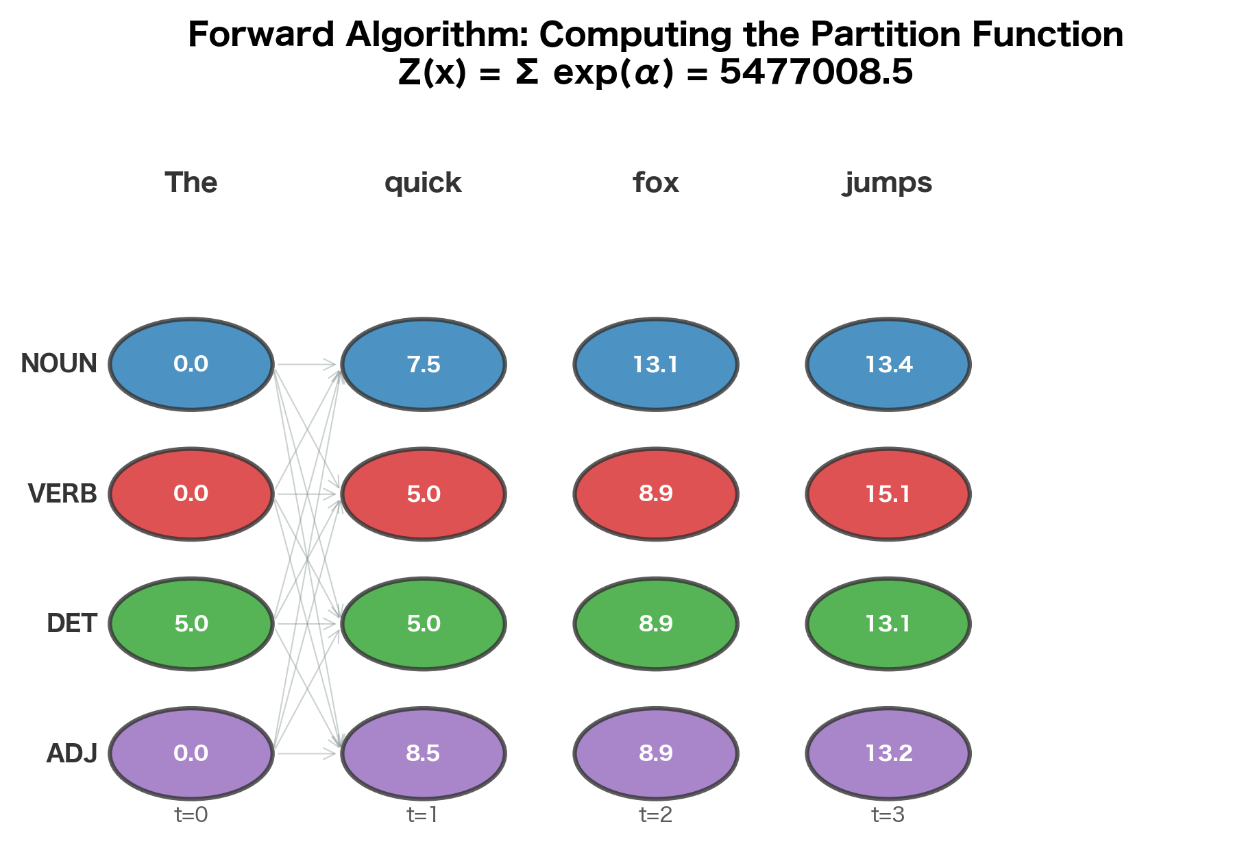
Computing the Partition Function
The partition function is the computational challenge of CRFs. It sums over all possible label sequences, and with labels and sequence length , there are such sequences. For labels and words, that's sequences, far too many to enumerate.

The Forward Algorithm
Fortunately, the linear-chain structure enables efficient computation via dynamic programming. The forward algorithm computes in time, similar to the forward algorithm for HMMs.
The key idea is to define a forward variable that accumulates scores for all partial label sequences ending in label at position :
where:
- : the forward variable at position for label
- : all possible label assignments for positions 1 through
- The sum aggregates scores over all ways to reach label at position
- The constraint fixes the label at position
Intuitively, represents the total "mass" of all paths that end in label at position . The crucial insight is that we can compute recursively from the previous position:
where:
- : iterates over all possible labels at position
- : the forward variable from the previous position
- : the score for transitioning from to at position
This recurrence says: to compute the total score of paths ending in at position , sum over all possible previous labels , multiplying the score of reaching by the score of the transition from to .
Once we've computed forward variables for all positions, the partition function is simply the sum over all labels at the final position:
where the sum is over all possible labels at the final position . This works because every complete label sequence must end with some label at position .
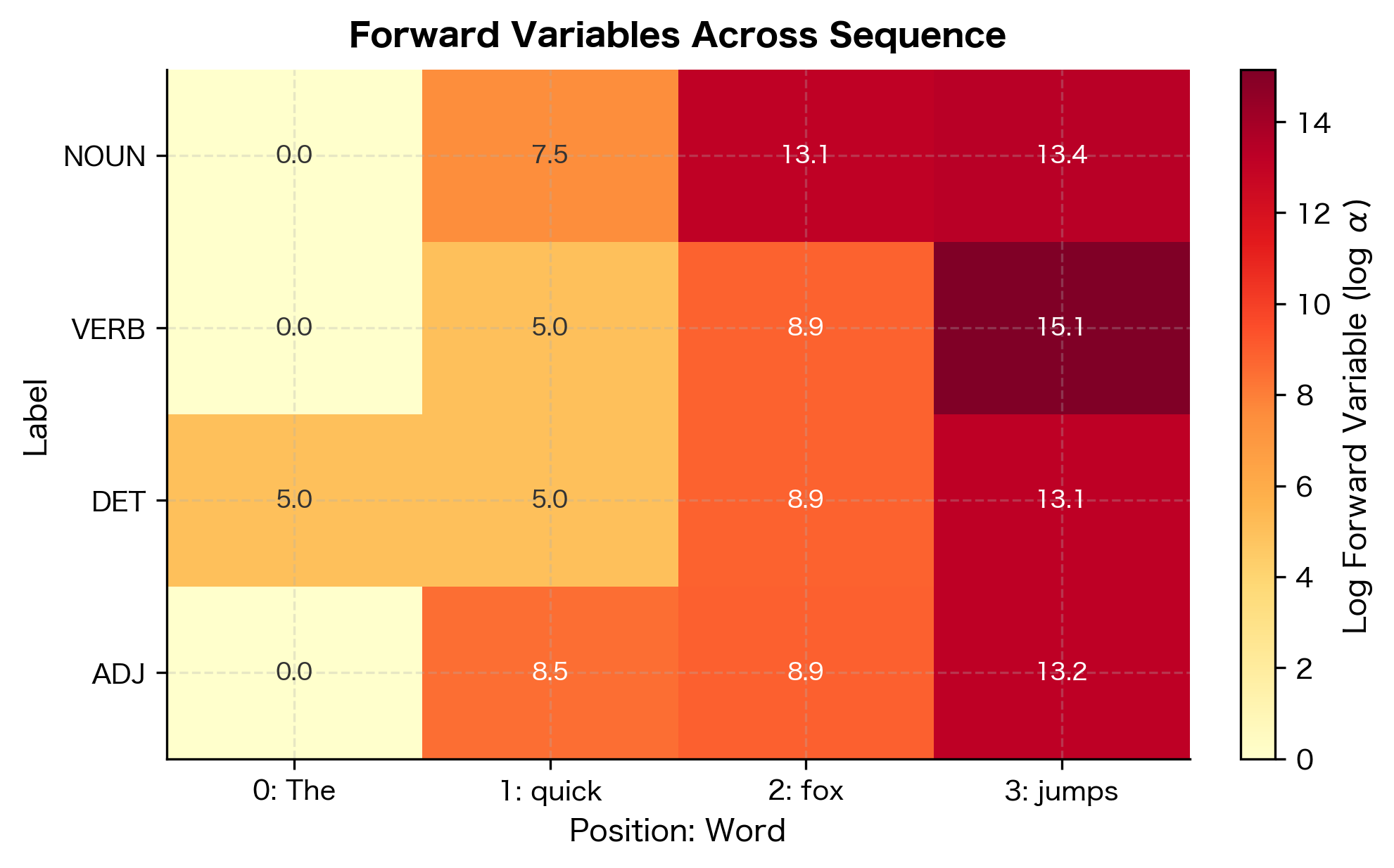
The forward variables show how probability mass accumulates through the sequence. At position 0, "The" has high scores for DET due to the matching feature weight. As we move through the sequence, the algorithm combines emission scores (how well each word matches each label) with transition scores (how likely each label sequence is). The log partition function aggregates all possible paths, enabling probability computation. Higher values indicate more probable label assignments at each position.
The forward algorithm exploits the linear-chain structure: at each position, we only need to consider transitions from labels at the previous position. This reduces the exponential enumeration to polynomial computation.
Log-Space Computation
Throughout CRF computations, we work in log space. Multiplying many probabilities (or exponentials of scores) quickly leads to numerical underflow. By using the log-sum-exp operation, we maintain numerical stability:
where:
- : the -th value we want to sum (in our case, log-scores for different label sequences)
- : the maximum value among all
- : the exponentiated value after subtracting the maximum
This identity is mathematically exact but numerically superior. The trick works because subtracting the maximum ensures that at least one term in the sum equals , while all other terms are less than 1. This prevents both overflow (from exponentiating large positive numbers) and underflow (from exponentiating large negative numbers).
CRF Inference with the Viterbi Algorithm
Training gives us feature weights. Inference finds the most likely label sequence for new observations:
where:
- : the optimal label sequence we want to find
- : "the value of that maximizes" the following expression
- : the conditional probability of label sequence given observations
- The double sum computes the total score for a candidate label sequence
The second equality holds because the partition function is constant for a given input. Since , and the exponential function is monotonically increasing, maximizing the probability is equivalent to maximizing the unnormalized score. The Viterbi algorithm, which you may know from HMMs, efficiently finds this maximum-scoring path.
The Viterbi algorithm has the same complexity as the forward algorithm. At each position, it tracks the best path to each label rather than summing all paths. Backpointers record which previous label led to the best score, enabling reconstruction of the optimal sequence.
Building a CRF Tagger with sklearn-crfsuite
Now let's build a practical CRF tagger using the sklearn-crfsuite library, which provides an efficient implementation with all the features we've discussed.
Now let's train the CRF model:
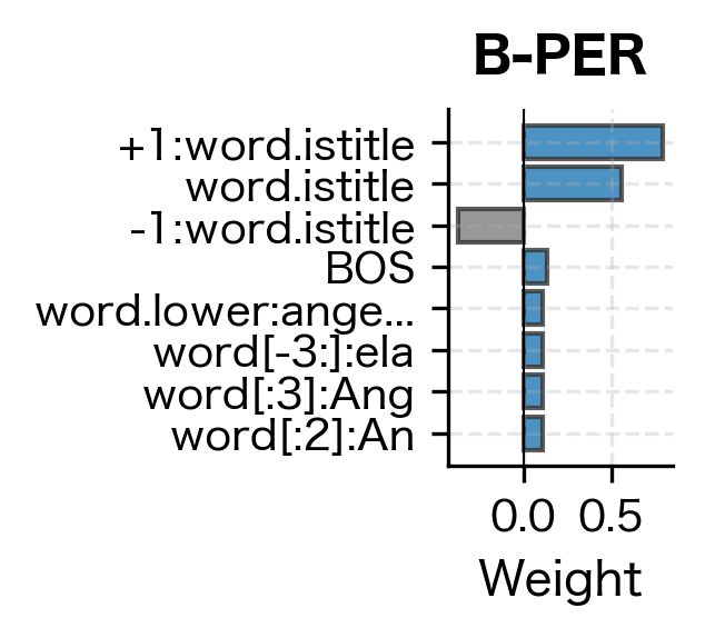
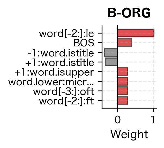
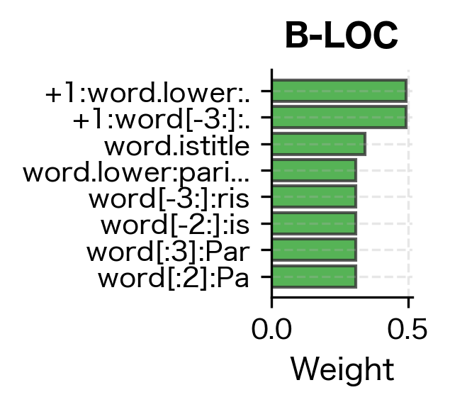
Even with minimal training data, the CRF correctly identifies person names (Tim Cook, with B-PER and I-PER tags) and organizations (Amazon as B-ORG). The model generalizes from the training examples by learning that capitalized words following patterns similar to training entities are likely named entities. Let's examine what features it learned to value:
The feature weights reveal what patterns the CRF learned to associate with each entity type. High positive weights indicate strong evidence for that label. Features like word.istitle (capitalization) and specific word forms from the training data carry the most weight, which aligns with our intuition that named entities are typically capitalized and follow predictable patterns.
Learned Transition Weights
CRFs also learn transition patterns between labels. Let's examine them:
The transition weights show strong preferences for valid BIO sequences. Transitions from B-tags to their corresponding I-tags have high positive weights, encouraging entity continuation. Transitions between different entity types (like B-PER to I-ORG) are penalized with negative weights, enforcing the constraint that I-tags must follow their matching B-tag.
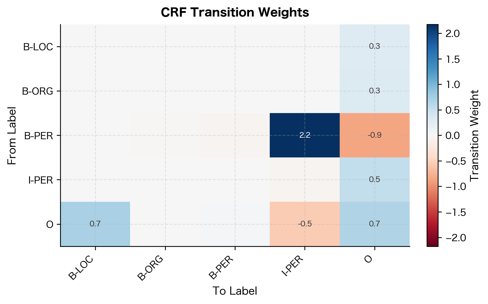
The transition weights reveal what the model learned about valid sequences. High positive weights between B-TYPE and I-TYPE labels encourage entity continuation. Negative weights for invalid transitions (like B-PER to I-LOC) discourage label sequences that violate BIO constraints.
CRF for Named Entity Recognition
Let's build a more complete NER system using a larger dataset. We'll use the CoNLL-2003 format, a standard for NER evaluation.
The per-entity metrics show how well the CRF recognizes each entity type. Precision measures how many predicted entities are correct, while recall measures how many actual entities were found. The F1 score balances both. Performance varies by entity type, with some entities being easier to recognize due to more distinctive features or more training examples.
The sample predictions show the CRF in action on real text. Checkmarks indicate correct predictions, while crosses highlight errors. Common error patterns include confusing similar entity types or missing entity boundaries, especially for entities not well-represented in training data.
Neural CRF Layers
Modern sequence labeling combines neural networks with CRF layers. The neural network learns feature representations, while the CRF layer models label dependencies and ensures valid output sequences.
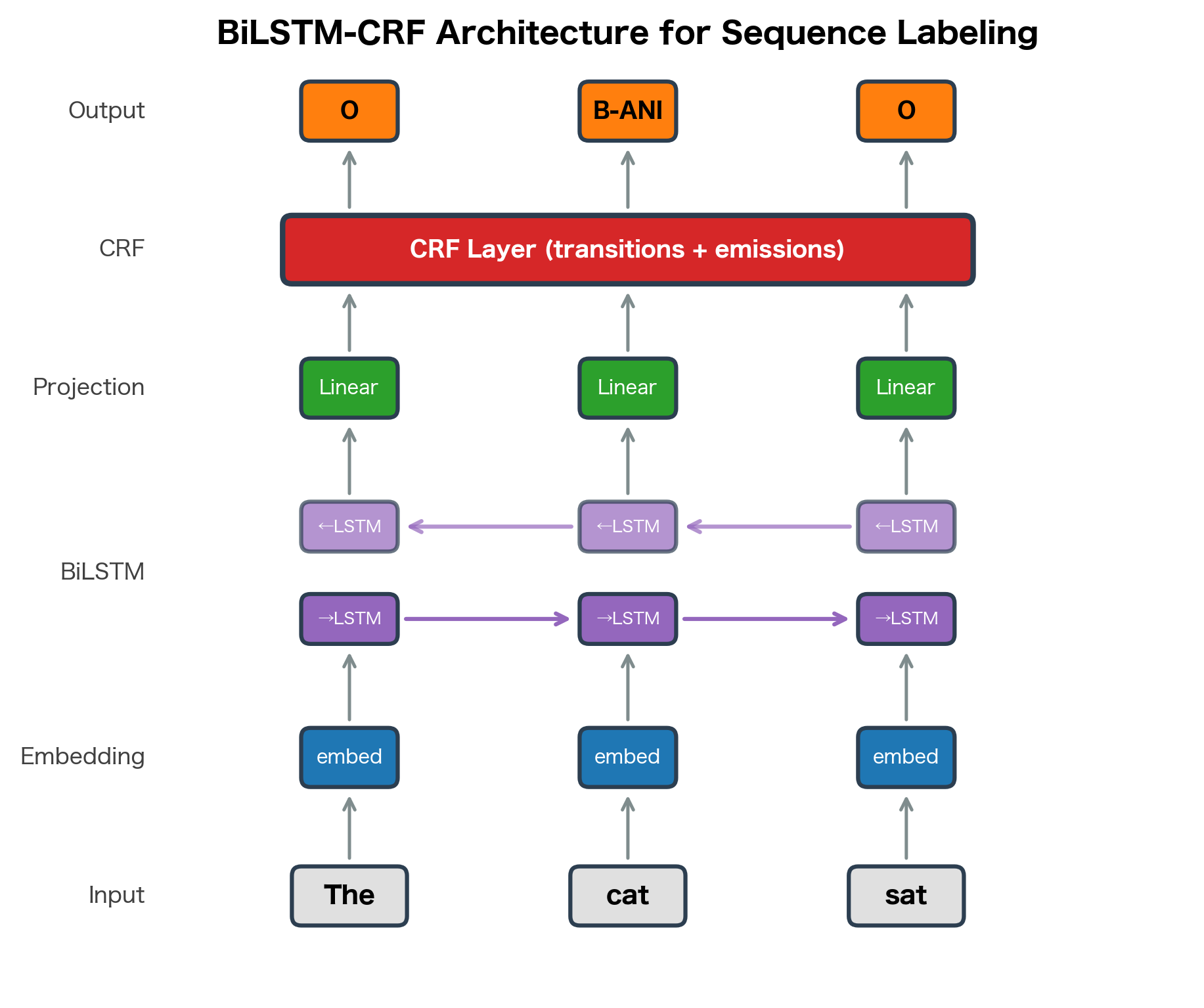
The BiLSTM-CRF architecture uses a bidirectional LSTM to encode contextual representations of each token, then feeds these representations to a CRF layer that models transition constraints between labels. The LSTM learns features; the CRF learns structure.
In this architecture:
- Word embeddings represent each token as a dense vector
- A BiLSTM processes the sequence, producing hidden states that capture bidirectional context
- A linear layer projects hidden states to label scores (emission scores)
- The CRF layer combines emission scores with learned transition scores
The CRF layer adds a transition matrix where is the score for transitioning from label to label . During training, we maximize the log-likelihood of correct label sequences. During inference, Viterbi decoding finds the best sequence.
The CRF layer computes three key quantities. The log partition function sums over all possible tag sequences (exponentially many), computed efficiently via the forward algorithm. The sequence score measures how well a specific tag sequence fits the emission and transition scores. The negative log-likelihood (the training loss) is the difference between these: minimizing it encourages the model to assign high scores to correct sequences relative to all alternatives. Viterbi decoding finds the highest-scoring path for inference.
The neural CRF combines the representation learning power of neural networks with the structured prediction capabilities of CRFs. The neural network extracts features automatically from the input, while the CRF layer ensures that the output sequence satisfies structural constraints like valid BIO transitions.
Inference Complexity and Practical Considerations
CRF inference has specific computational characteristics worth understanding for practical applications.
Time Complexity
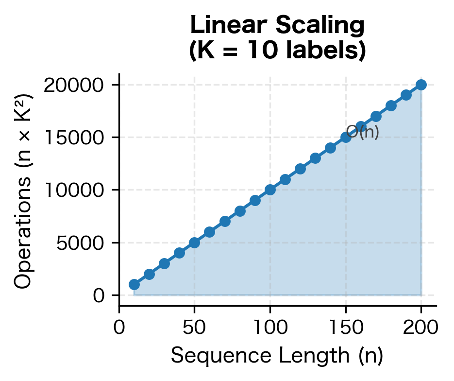
The key operations scale as follows:
- Forward/Backward Algorithm: where is sequence length and is number of labels
- Viterbi Decoding:
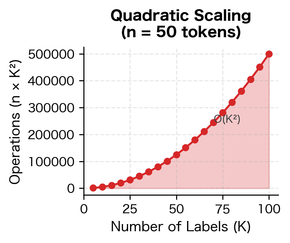
- Gradient Computation: per training example
The quadratic dependence on means that CRFs become expensive with many labels. For tasks with hundreds of possible labels (like fine-grained NER with many entity types), this can be a bottleneck.
Beam Search Alternative
When exact Viterbi decoding is too slow, beam search provides an approximate alternative. Instead of tracking all labels at each position, beam search keeps only the top partial sequences:
Beam search with width 1 is greedy decoding. As beam width increases, accuracy approaches Viterbi but with reduced computational cost for very long sequences or many labels.
Limitations and When CRFs Fall Short
Despite their power, CRFs have limitations that have driven the development of alternative approaches:
-
Label Set Size: The complexity becomes prohibitive with large label sets. Tasks with hundreds of labels, such as fine-grained entity typing or word sense disambiguation, may require approximations or alternative architectures. Hierarchical CRFs and sparse transition matrices can help, but fundamentally, CRFs work best with modest numbers of labels.
-
Long-Range Dependencies: Linear-chain CRFs model only adjacent label dependencies. If a label at position 10 directly depends on the label at position 1, the CRF cannot capture this except through a chain of intermediate influences. Higher-order CRFs exist but are exponentially more expensive. For tasks requiring long-range dependencies, attention mechanisms in transformers often work better.
-
Feature Engineering: Traditional CRFs require manual feature engineering. While neural CRFs learn features automatically, they add the complexity of neural network training: hyperparameter tuning, GPU requirements, and longer training times. For some applications, a well-engineered feature-based CRF may outperform a neural CRF with less effort.
-
Training Data Requirements: CRFs need labeled sequences for training. Unlike language models that can pretrain on unlabeled text, CRF features and transitions are learned entirely from labeled data. This makes them data-hungry for complex tasks. The combination of pretrained transformers with CRF layers addresses this by providing rich features from unlabeled pretraining.
These limitations don't diminish CRFs' importance. They remain the go-to structured prediction layer for sequence labeling, especially in production systems where interpretable features and reliable inference matter. Understanding both their strengths and limitations helps you choose the right tool for each problem.
Key Parameters
When working with CRFs using sklearn-crfsuite, the following parameters most significantly affect model performance:
-
algorithm: The optimization algorithm for training. Options include"lbfgs"(Limited-memory BFGS, default),"l2sgd"(SGD with L2 regularization),"ap"(Averaged Perceptron), and"pa"(Passive Aggressive). L-BFGS typically converges faster and works well for most tasks. SGD variants may be preferred for very large datasets that don't fit in memory. -
c1(L1 regularization): Controls feature sparsity. Higher values push more feature weights to exactly zero, producing simpler models with fewer active features. Start with values between 0.0 and 0.5. Useful when you have many features and want automatic feature selection. -
c2(L2 regularization): Controls weight magnitude. Higher values prevent any single feature from dominating predictions. Start with values between 0.01 and 0.1. Helps prevent overfitting, especially with limited training data. -
max_iterations: Maximum number of optimization iterations. Default is 100, which suffices for most tasks. Increase if the model hasn't converged (check training logs). Very large values rarely help and slow training. -
all_possible_transitions: WhenTrue, includes transition weights for all label pairs, even those not observed in training. This allows the model to learn that unseen transitions should have negative weights. Generally recommended for BIO tagging where you want to explicitly penalize invalid transitions like B-PER to I-LOC. -
all_possible_states: WhenTrue, includes state features for all labels, even for features not observed with that label in training. Useful when test data may contain feature-label combinations not seen during training.
For neural CRFs, key parameters include the hidden dimension of the LSTM (typically 64-256), dropout rate (0.1-0.5), and learning rate (1e-4 to 1e-3 with Adam optimizer).
Summary
Conditional Random Fields represent a fundamental advance in sequence labeling, shifting from generative to discriminative modeling to unlock richer feature representations.
Key concepts from this chapter:
Generative vs. Discriminative: HMMs model and derive predictions through Bayes' rule. CRFs directly model , avoiding independence assumptions about observations. This allows arbitrary overlapping features of the input sequence.
Log-Linear Formulation: CRFs define probabilities through weighted feature functions:
where is the label sequence, is the observation sequence, are learned weights, are feature functions, and normalizes the distribution. Feature functions capture both label-observation relationships (like HMM emissions) and label-label relationships (like HMM transitions), plus arbitrary combinations.
Partition Function: The normalization constant sums over all possible label sequences. The forward algorithm computes it efficiently in time using dynamic programming.
Inference: The Viterbi algorithm finds the most likely label sequence in time. Beam search provides an approximate alternative for very large label sets.
Feature Functions: CRF power comes from rich features:
- State features link observations to labels (word suffixes, capitalization, POS tags)
- Transition features capture label-label patterns (valid BIO transitions)
- Context features use surrounding words and their properties
Neural CRFs: Modern architectures combine neural networks (BiLSTMs, transformers) for feature learning with CRF layers for structured prediction. The neural network learns representations; the CRF enforces output constraints.
Implementation: Libraries like sklearn-crfsuite provide efficient CRF training and inference. Feature engineering remains important for traditional CRFs, while neural CRFs learn features automatically but require more training infrastructure.
CRFs transformed sequence labeling by providing a principled framework for combining rich, overlapping features with structured output constraints. They remain the foundation of production NER, POS tagging, and chunking systems, either as traditional feature-based models or as structured output layers in neural architectures. The next chapter explores CRF training in detail: the forward-backward algorithm, gradient computation, and optimization techniques that make learning possible.
Quiz
Ready to test your understanding? Take this quick quiz to reinforce what you've learned about Conditional Random Fields and discriminative sequence labeling.

Comments