

Learn how stacking multiple RNN layers creates deep networks for hierarchical representations. Covers residual connections, layer normalization, gradient flow, and practical depth limits.

This article is part of the free-to-read Language AI Handbook
Choose your expertise level to adjust how many terms are explained. Beginners see more tooltips, experts see fewer to maintain reading flow. Hover over underlined terms for instant definitions.
Stacked RNNs
In the previous chapters, we've explored how individual recurrent layers process sequences. A single LSTM or GRU layer learns to capture patterns at one level of abstraction, transforming raw inputs into hidden representations that encode temporal dependencies. But just as convolutional neural networks benefit from stacking multiple layers to capture increasingly abstract visual features, recurrent networks can be stacked to learn hierarchical representations of sequential data.
Stacked RNNs, also called deep RNNs, connect multiple recurrent layers vertically. The output sequence from one layer becomes the input to the next, allowing each successive layer to operate on increasingly refined representations. The first layer might learn low-level patterns like word boundaries or phonemes, while deeper layers capture higher-level structures like phrases, sentences, or semantic relationships. This hierarchical processing has proven essential for complex sequence tasks like machine translation, speech recognition, and language modeling.
The Case for Depth
Before diving into architecture details, let's understand why depth matters for sequence modeling. A single recurrent layer has limited representational capacity. It must simultaneously handle multiple responsibilities: encoding the input, maintaining memory of past information, and producing useful outputs. Stacking layers allows these responsibilities to be distributed across a hierarchy.
Consider language understanding. At the lowest level, you need to recognize individual words and their immediate contexts. At a higher level, you need to understand phrase structures and grammatical relationships. At the highest level, you need to grasp document-level themes and long-range coherence. A single RNN layer struggles to capture all these levels simultaneously, but a stacked architecture can dedicate different layers to different abstraction levels.
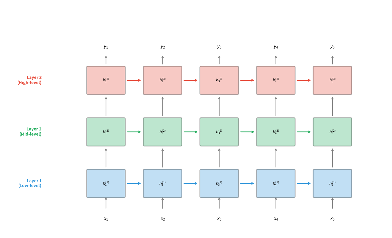
The figure shows how information flows in a stacked RNN. Each layer maintains its own sequence of hidden states, with information flowing both horizontally (across time within a layer) and vertically (from lower to higher layers at each timestep). This creates a grid of computations where each cell depends on both its temporal predecessor and its hierarchical predecessor.
Mathematical Formulation
Now that we understand why depth matters, enabling hierarchical feature extraction where different layers capture different levels of abstraction, let's formalize how information actually flows through a stacked RNN. Our goal is to derive the equations that govern computation at each layer, understanding not just what they say but why they take the form they do.
The Core Question: What Does Each Layer Receive?
The fundamental insight behind stacked RNNs is simple: each layer should process increasingly refined representations. But this raises a concrete question: if layer 1 processes the raw input, what exactly should layer 2 process?
Consider the alternatives:
-
Same input: Every layer receives . But this would mean all layers are doing essentially the same job, with no hierarchy.
-
Accumulated output: Layer receives all outputs from layers below. This creates redundancy and computational overhead.
-
Output from layer below: Layer receives only the hidden state from layer at the same timestep. This is elegant because each layer refines what the previous layer produced.
The third option is what stacked RNNs use. It creates a natural hierarchy: layer 1 transforms raw features into initial patterns, layer 2 transforms those patterns into higher-level structures, and so on. Each layer has a single, focused job: refine the representation from below.
The First Layer: Processing Raw Input
The first layer operates exactly like a standard RNN. At each timestep , it combines two sources of information:
- The current input , representing what's happening now
- The previous hidden state , representing what happened before
The superscript denotes "layer 1." The computation is:
Let's unpack each component and understand its role:
| Symbol | Shape | Role |
|---|---|---|
| Output: layer 1's hidden state at time | ||
| Temporal memory: what layer 1 remembers from time | ||
| Current input features (e.g., word embedding) | ||
| Recurrent weights: how past hidden state influences present | ||
| Input weights: how current input projects to hidden dimension | ||
| Bias: learned offset for each hidden unit | ||
| - | Activation function (tanh, or full LSTM/GRU computation) |
The matrix multiplication transforms the -dimensional input into the -dimensional hidden space. Meanwhile, transforms the previous hidden state, allowing temporal information to flow forward. The sum of these two terms, plus bias, passes through the activation function to produce the new hidden state.
You might wonder why we use separate matrices and rather than concatenating and using a single matrix. Mathematically, they're equivalent. But separating them clarifies the two distinct roles: handles temporal dynamics (how the past influences the present), while handles input processing (how new information enters the system). This separation also makes it easier to analyze and initialize each component appropriately.
Subsequent Layers: Refining Representations
Here's where the stacked architecture becomes interesting. For layer , we make a single but crucial change: instead of receiving the raw input , layer receives the hidden state from the layer below at the same timestep. The equation becomes:
The only difference from layer 1 is that has been replaced by . Let's examine what this means:
| Symbol | Shape | Role |
|---|---|---|
| Output: layer 's hidden state at time | ||
| Temporal memory within layer (horizontal flow) | ||
| Input from layer at same timestep (vertical flow) | ||
| Recurrent weights for layer | ||
| Input weights for layer (note: now , not ) | ||
| Bias for layer |
Notice that is now rather than . This is because the "input" to layer is no longer the raw features. It's the hidden state from the layer below, which already has dimension .
Two Dimensions of Information Flow
The stacked architecture creates a two-dimensional grid of computations. At each cell , representing timestep and layer , information flows from two sources:
-
Horizontal (temporal): From , the same layer's hidden state at the previous timestep. This captures sequential dependencies within each abstraction level.
-
Vertical (hierarchical): From , the layer below at the same timestep. This enables hierarchical feature extraction.
This dual flow is what gives stacked RNNs their power. Layer 1 might learn to recognize that "not" followed by "good" signals something different than "good" alone (temporal pattern). Layer 2 might learn to recognize that this negation pattern, combined with certain sentence structures, indicates sarcasm (hierarchical abstraction built on layer 1's output).
A Concrete Example: Processing a Sentence
Let's trace how a 3-layer stacked RNN processes the sentence "The cat sat." Assume:
- Vocabulary size: 1000 words
- Embedding dimension
- Hidden size
- Each word is represented by a 64-dimensional embedding
At timestep 1 ("The"):
- Layer 1 receives (embedding of "The") and (initialized to zeros)
- Layer 1 produces : a 128-dim vector encoding "The" in context
- Layer 2 receives and (zeros)
- Layer 2 produces : a more abstract representation
- Layer 3 receives and (zeros)
- Layer 3 produces : the highest-level representation
At timestep 2 ("cat"):
- Layer 1 receives (embedding of "cat") and (encodes "The")
- Layer 1 produces : encodes "The cat" at a basic level
- Layer 2 receives and
- Layer 2 produces : recognizes this is likely a noun phrase
- Layer 3 receives and
- Layer 3 produces : captures high-level semantic content
The pattern continues for "sat." By the final timestep, contains a hierarchically processed representation of the entire sentence, with low-level word patterns, mid-level phrase structures, and high-level semantic meaning all encoded.
In a stacked RNN, only the first layer sees the raw input . All subsequent layers take the hidden state from the layer below as their "input." This means layer 2 processes the sequence of hidden states , layer 3 processes , and so on.
Implementing Stacked RNNs in PyTorch
With the mathematical foundation in place, let's translate these equations into working code. We'll explore two approaches: building a stacked RNN manually layer-by-layer, and using PyTorch's built-in num_layers parameter. Understanding both will deepen your intuition for how the architecture works.
Approach 1: Manual Layer Stacking
The most instructive way to understand stacked RNNs is to build one explicitly. We'll create a ModuleList of individual LSTM layers and connect them ourselves:
Notice the key detail in the constructor: the first layer has input_size as its input dimension (matching the raw features), while all subsequent layers have hidden_size as their input dimension (because they receive the hidden state from the layer below). This is exactly what our mathematical formulation prescribed. Layer 1 processes with shape , while layers process with shape .
The forward method implements the vertical information flow we described: each layer's output becomes the next layer's input. The _ = layer(x) discards the final hidden state tuple, keeping only the sequence of outputs.
Approach 2: Built-in num_layers Parameter
PyTorch provides a more concise way to create the same architecture:
This single nn.LSTM with num_layers=3 is functionally equivalent to our manual implementation with three separate layers. PyTorch handles the inter-layer connections internally.
Verifying Equivalence
Let's confirm that both approaches produce the same output structure:
Both models transform a (4, 20, 32) input into a (4, 20, 64) output. The input has 32 features per timestep; after passing through 3 LSTM layers, each with hidden size 64, we get 64-dimensional hidden states at each of the 20 timesteps. Importantly, the output contains only the final layer's hidden states. The intermediate layers' outputs are used internally but not returned by default.
When to Use Each Approach
The built-in num_layers approach is generally preferred for production code:
- Performance: PyTorch can optimize the computation using cuDNN, fusing operations across layers for faster execution on GPUs
- Simplicity: Less code means fewer bugs and easier maintenance
- Dropout integration: The built-in version supports inter-layer dropout via the
dropoutparameter
The manual approach is valuable when you need:
- Different hidden sizes per layer: Perhaps layer 1 has 256 units while layer 3 has 64
- Different cell types: Maybe you want LSTM for layer 1 and GRU for layer 2
- Custom inter-layer processing: Adding normalization, attention, or other operations between layers
- Access to intermediate outputs: Extracting hidden states from each layer, not just the final one
We'll use the manual approach later when adding residual connections, since those require explicit access to each layer's input and output.
Depth vs Width Trade-offs
A fundamental question when designing stacked RNNs is whether to go deeper (more layers) or wider (larger hidden sizes). Both increase model capacity, but they do so in different ways with distinct computational and learning implications.
| Configuration | Layers | Hidden | Parameters |
|---|---|---|---|
| 1 layer, h=512 | 1 | 512 | ~1.3M |
| 2 layers, h=362 | 2 | 362 | ~1.3M |
| 3 layers, h=296 | 3 | 296 | ~1.4M |
| 4 layers, h=256 | 4 | 256 | ~2.0M |
The parameter counts reveal an interesting pattern: you can achieve similar model capacity through different architectural choices. A single layer with 512 hidden units has roughly 1.3 million parameters, while a 4-layer network with 256 hidden units has about 2 million. The deeper network has more parameters due to the inter-layer connections, but both are in the same order of magnitude.
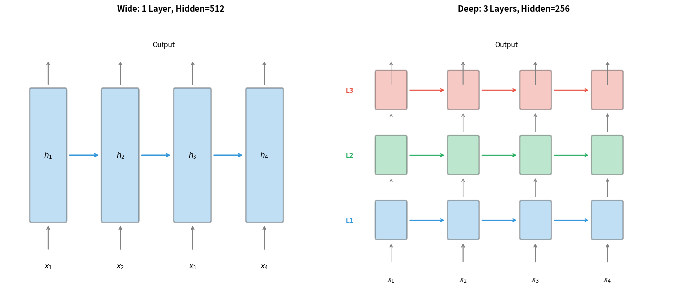
The representational properties differ significantly despite similar capacities:
-
Wide networks have more capacity at each timestep but limited hierarchical processing. They're better when you need to capture complex patterns at a single level of abstraction.
-
Deep networks can learn hierarchical representations but require careful training. They're better when your data has natural hierarchical structure, like language with its levels of words, phrases, and sentences.
In practice, the optimal choice depends on your task. Machine translation systems often use 4-8 LSTM layers, finding that depth helps capture the complex transformations between languages. Language models typically use 2-4 layers, as excessive depth can hurt perplexity. Speech recognition systems often go deeper (6+ layers) because audio has natural hierarchical structure from phonemes to words to phrases.
To understand the trade-off more precisely, let's examine how parameters scale with depth versus width:
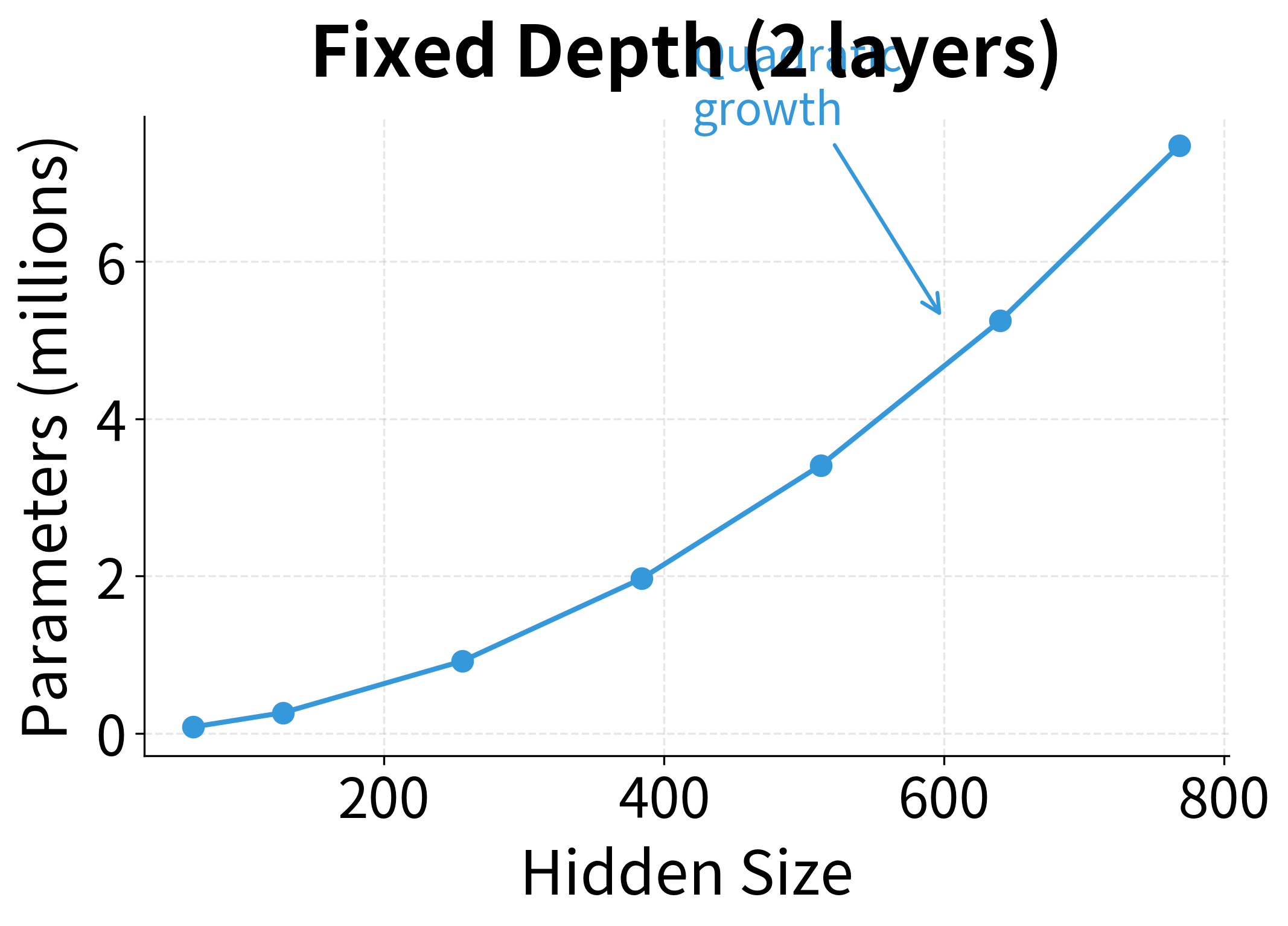
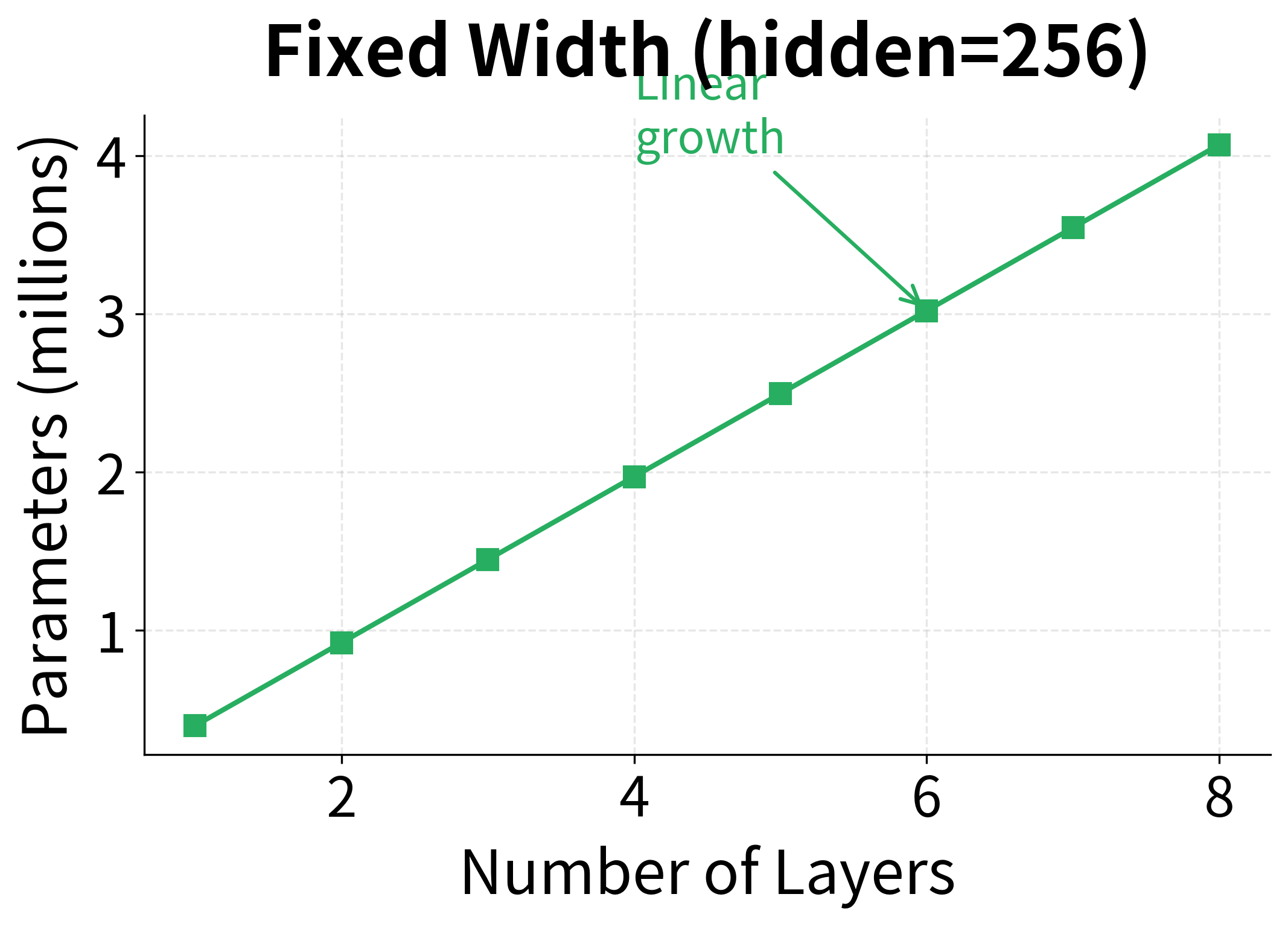
The scaling behavior reveals why deep networks can be more parameter-efficient: doubling the hidden size roughly quadruples the parameters (since LSTM weights scale as ), while doubling the depth only doubles them. However, deeper networks are harder to train and have higher latency per timestep, so the optimal trade-off depends on your computational constraints and task requirements.
Gradient Flow in Deep RNNs
Stacking RNN layers introduces a new challenge: gradients must flow not only backward through time but also downward through layers. This creates two orthogonal paths for gradient propagation, each with its own potential for vanishing or exploding gradients.
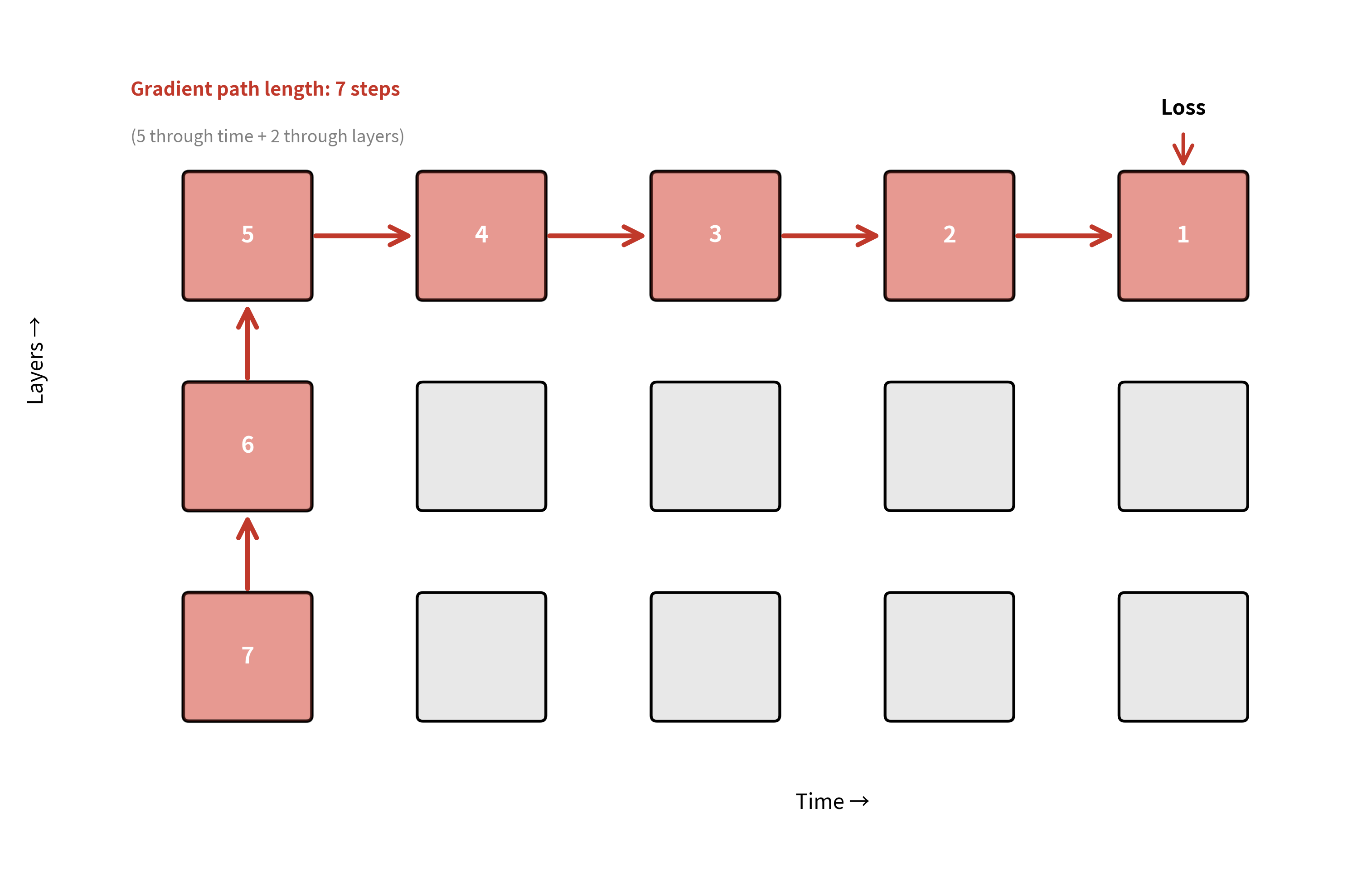
The total gradient path length from the loss to the first timestep of the first layer is , where:
- : the sequence length (number of timesteps)
- : the number of layers in the stack
For a 100-timestep sequence with 4 layers, gradients must traverse steps. Even with LSTMs mitigating temporal gradient issues, the vertical gradient flow through layers can still cause problems.
Let's simulate how gradient magnitude changes as we add more layers:
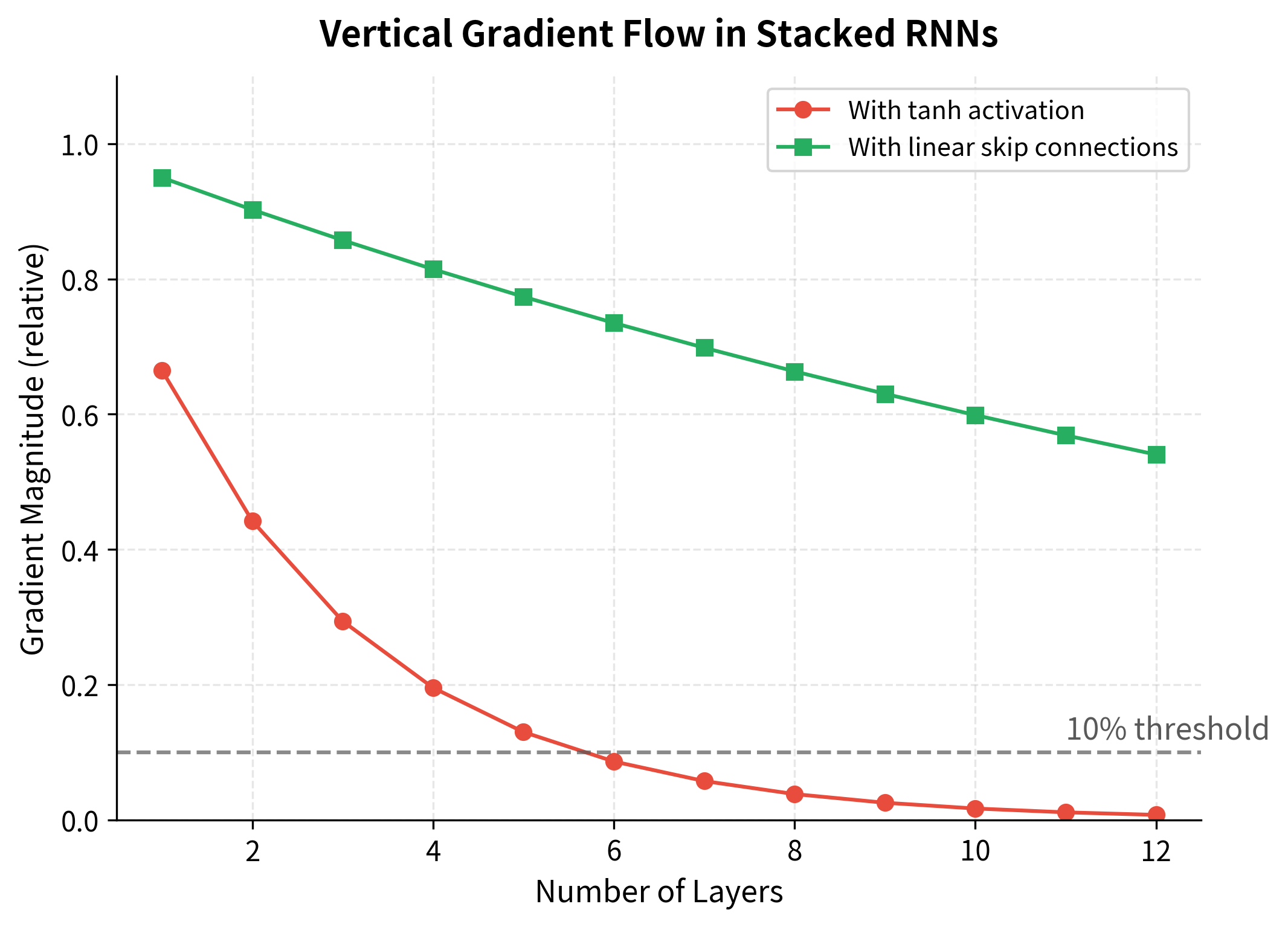
The simulation shows that with standard tanh activations, gradients decay to less than 10% of their original magnitude after just 4-5 layers. This vertical gradient decay compounds with the temporal gradient issues we discussed in earlier chapters. The solution lies in architectural modifications that provide direct gradient pathways through the network: residual connections.
Residual Connections for Depth
Residual connections, introduced by He et al. in their ResNet paper for image classification, have become essential for training deep RNNs. The idea is simple: instead of learning a transformation , learn a residual . This creates a direct path for gradients to flow backward without passing through nonlinearities.
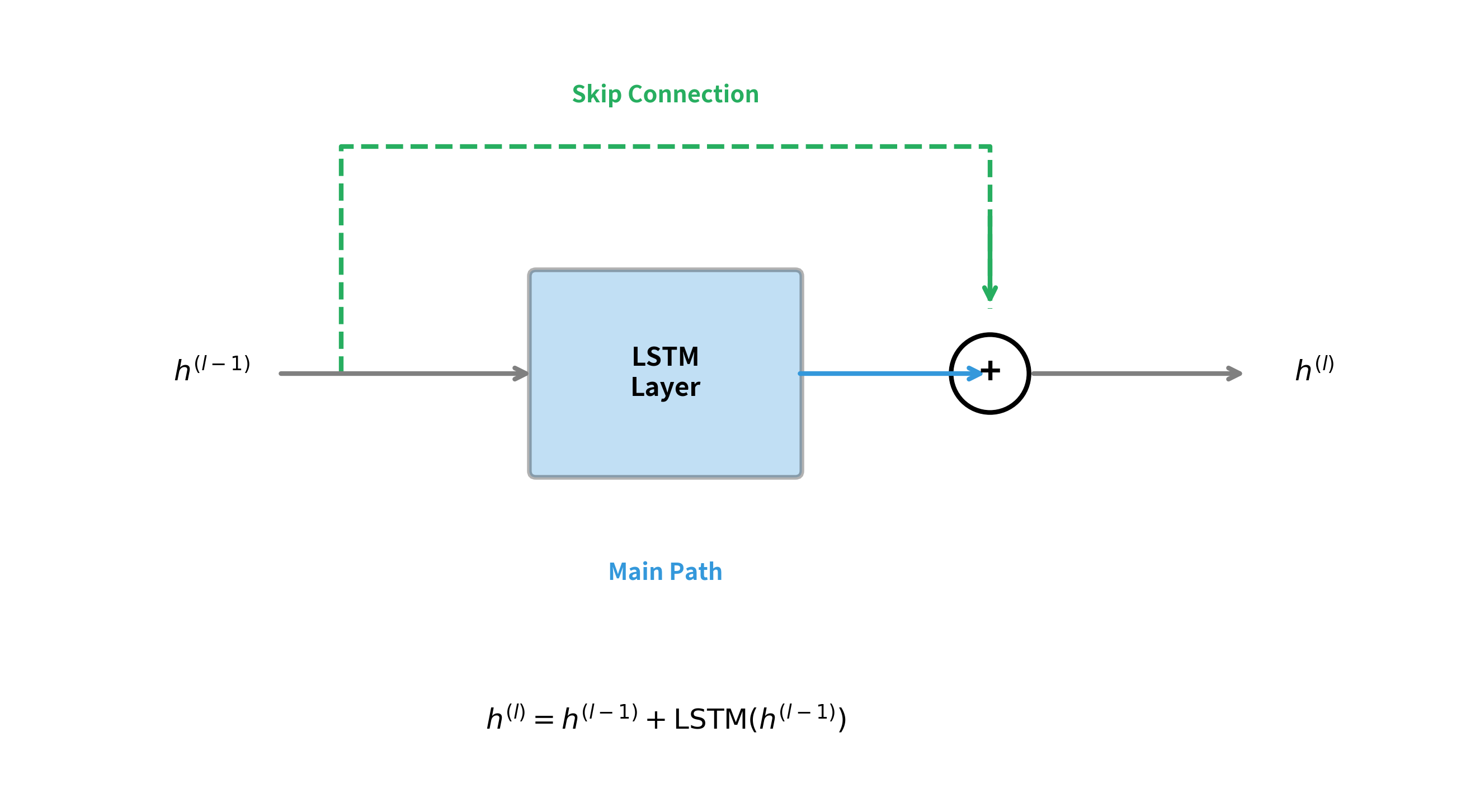
The mathematical formulation for a residual stacked RNN layer adds the input directly to the output of the RNN transformation:
where:
- : output hidden state of layer at timestep
- : input to layer (output from layer below), which is added directly via the skip connection
- : the RNN transformation at layer , taking both the input from below and the previous hidden state
During backpropagation, we need to compute how the loss changes with respect to the input . Using the chain rule on the residual formula:
where:
- : the identity matrix, arising from the derivative of the skip connection term
- : the Jacobian of the RNN transformation with respect to its input
The identity matrix is the key to why residual connections work. Even if the RNN gradient term vanishes (approaches zero), the identity term ensures that gradients can still flow directly through the skip connection. This is the same principle that allows ResNets to train networks with hundreds of layers.
Let's implement a stacked LSTM with residual connections:
The difference is striking. The residual model maintains gradients that are hundreds of times larger than the standard stacked LSTM. This dramatic improvement comes from the skip connections providing a direct gradient pathway that bypasses the potentially vanishing gradients through the LSTM transformations. In practice, this means the first layer receives meaningful learning signals even in deep networks, enabling faster and more stable training.
Layer Normalization in RNNs
While batch normalization revolutionized training of feedforward networks, it doesn't work well for RNNs. The issue is that batch statistics vary across timesteps, and computing separate statistics for each timestep requires impractically large batches. Layer normalization, introduced by Ba et al. in 2016, provides an alternative that normalizes across features rather than across the batch.
Batch normalization normalizes across the batch dimension: for each feature, compute mean and variance across all samples in the batch. This requires large batches and consistent statistics across timesteps.
Layer normalization normalizes across the feature dimension: for each sample at each timestep, compute mean and variance across all features. This works with any batch size and handles variable-length sequences naturally.
Layer normalization transforms a hidden state vector by normalizing its values to have zero mean and unit variance, then applying a learned affine transformation. For a hidden state with dimension , the computation is:
where:
- : the input hidden state vector of dimension
- : the mean of all elements in , computed as
- : the variance of all elements in , computed as
- : a learned scale parameter vector of dimension , initialized to ones
- : a learned shift parameter vector of dimension , initialized to zeros
- : a small constant (typically ) added for numerical stability to prevent division by zero
- : element-wise multiplication
The normalization step centers the values around zero and scales them to unit variance. The learned parameters and then allow the network to undo this normalization if needed, giving the model flexibility while still benefiting from the stabilizing effects during training.
Layer normalization provides several benefits for stacked RNNs:
- Stabilizes activations: Prevents hidden states from growing unboundedly or collapsing to zero
- Reduces sensitivity to initialization: Networks train more reliably with different random seeds
- Enables larger learning rates: Normalized activations allow more aggressive optimization
- Improves generalization: Acts as a regularizer, reducing overfitting
Practical Depth Limits
Despite residual connections and layer normalization, there are practical limits to how deep RNNs can go. Unlike feedforward networks that can scale to hundreds of layers, RNNs typically max out at 4-8 layers for most applications. Let's explore why.
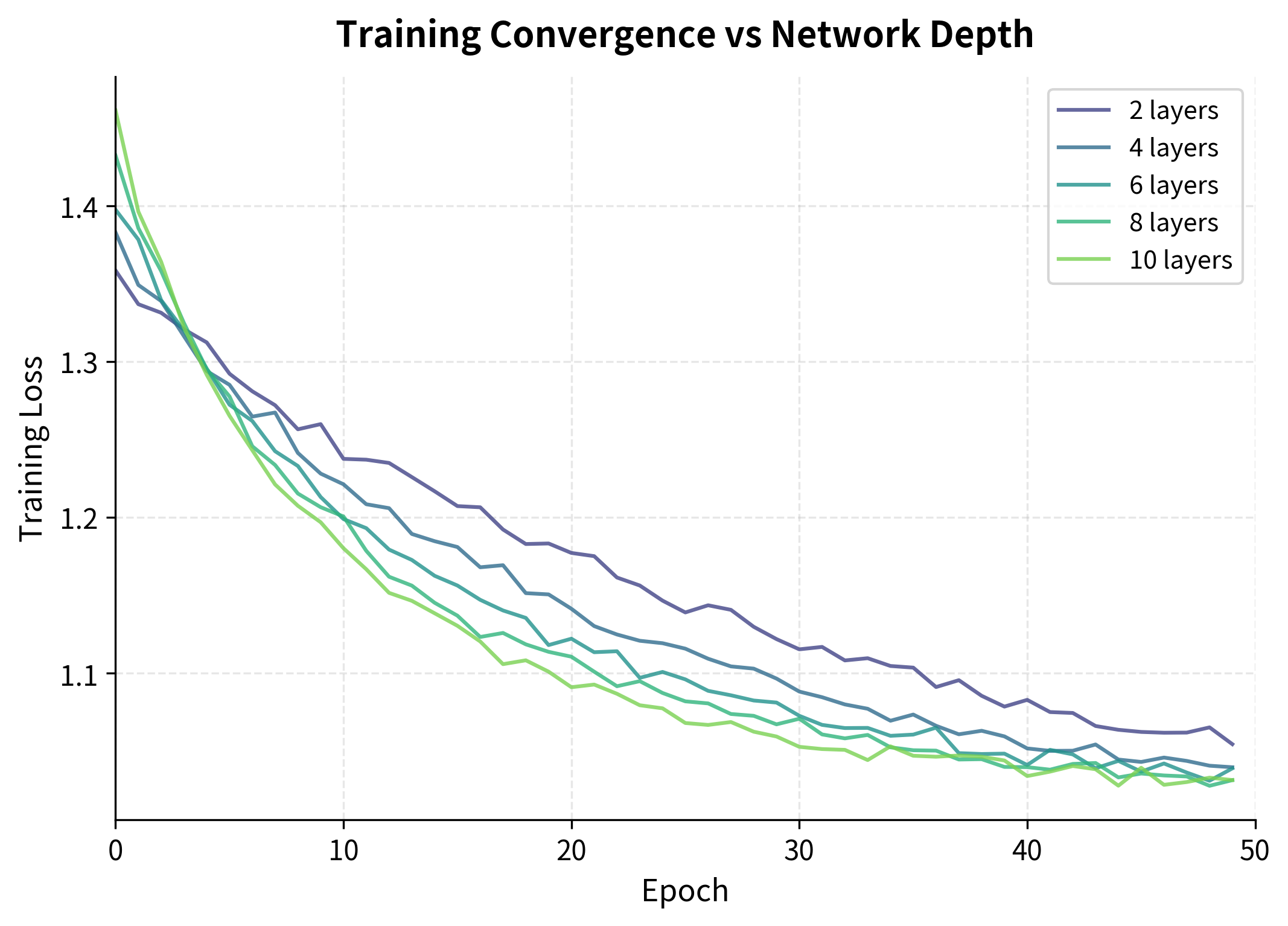
The training curves reveal several patterns. Shallower networks (2-4 layers) converge quickly and smoothly. Medium-depth networks (6-8 layers) can achieve lower final loss but take longer to converge. Very deep networks (10+ layers) often struggle with optimization, showing slower convergence and higher variance.
Several factors contribute to these practical depth limits:
-
Sequential computation overhead: Each layer adds latency. With 8 layers, you're doing 8 times the computation per timestep compared to a single layer.
-
Memory requirements: Storing hidden states for all layers at all timesteps during training grows as , where is the number of layers, is the sequence length, and is the hidden size.
-
Optimization difficulty: Even with residual connections, very deep networks have complex loss landscapes that are harder to navigate.
-
Diminishing returns: Beyond a certain depth, additional layers provide less representational benefit. The hierarchical structure of most data doesn't require arbitrarily deep processing.
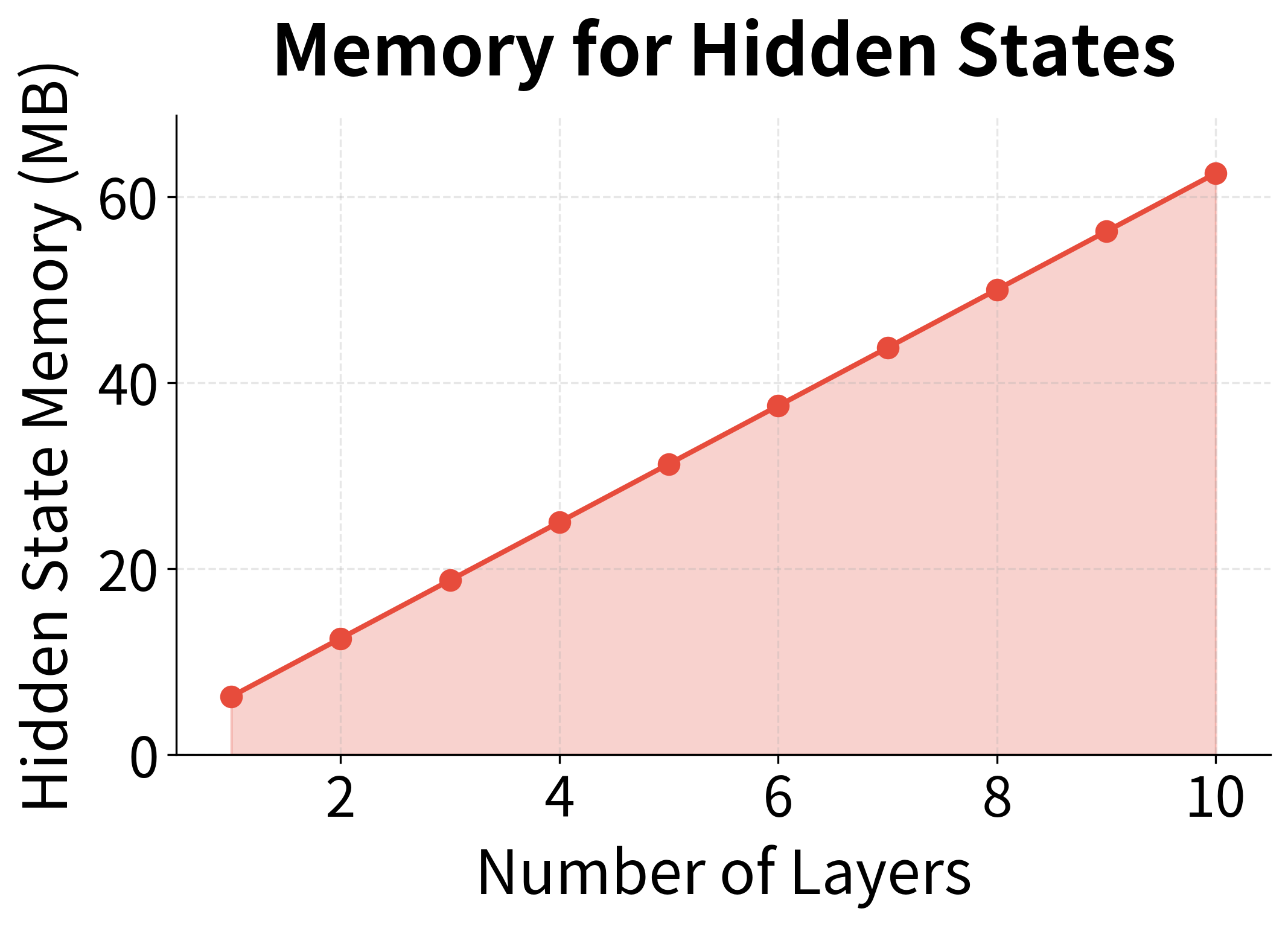
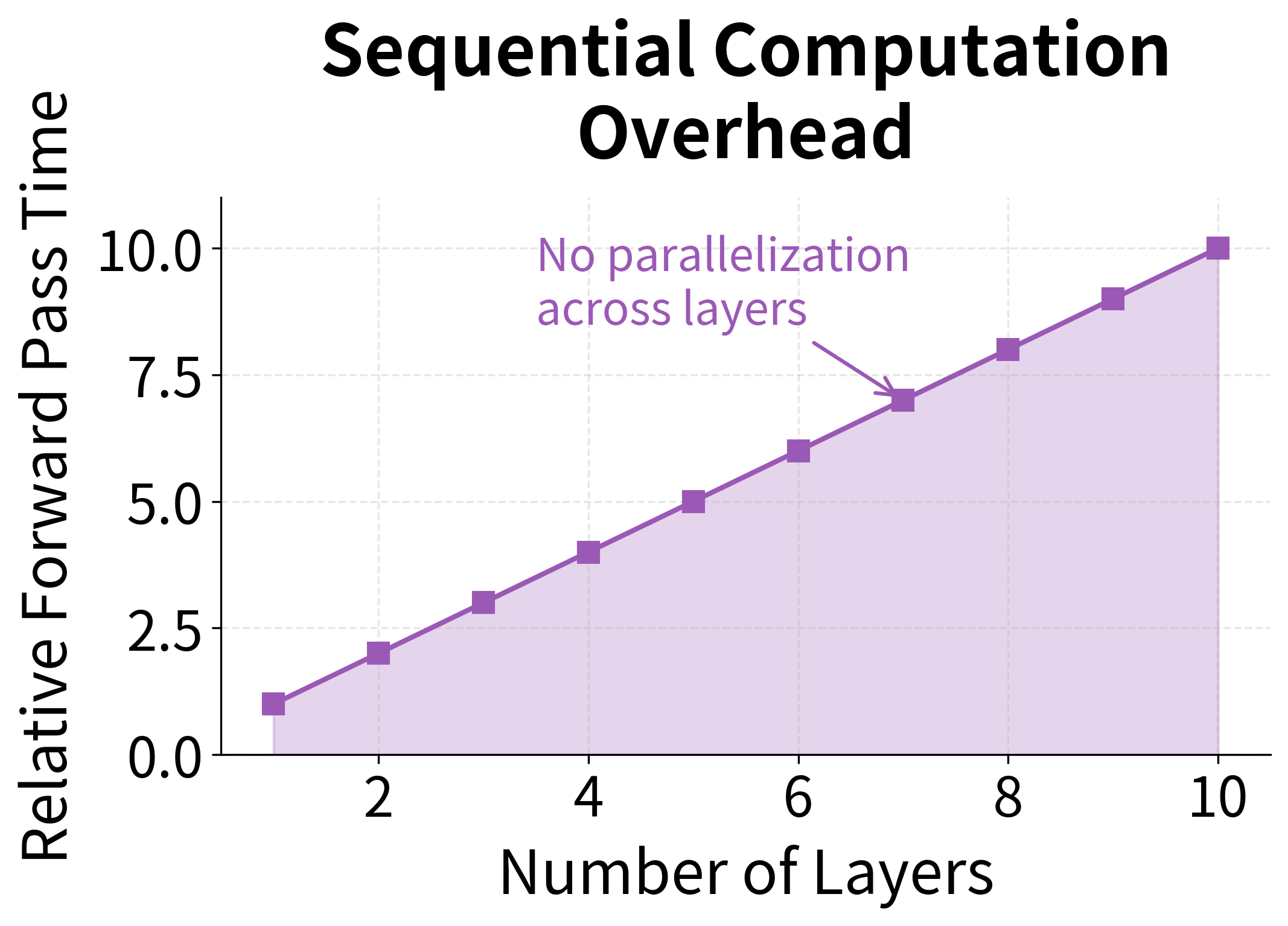
These scaling factors explain why practitioners rarely go beyond 6-8 layers. A 10-layer network requires 10× the memory for hidden states and 10× the forward pass time compared to a single layer, but typically provides only marginal improvements in task performance.
| Task | Typical Depth | Rationale |
|---|---|---|
| Language modeling | 2-4 layers | Diminishing perplexity gains beyond 4 layers |
| Machine translation | 4-8 layers | Complex transformations benefit from depth |
| Speech recognition | 5-7 layers | Hierarchical audio structure |
| Sentiment analysis | 2-3 layers | Simple classification doesn't need depth |
| Sequence labeling | 2-4 layers | Per-token decisions are relatively local |
Putting It All Together: A Complete Implementation
Let's build a production-ready stacked RNN that incorporates all the techniques we've discussed: multiple layers, residual connections, layer normalization, and dropout. This architecture represents current best practices for deep recurrent networks.
The model has approximately 542,000 parameters, which is reasonable for a 4-layer network with hidden size 128. Each layer maintains the same output shape (8, 50, 128) because we use residual connections that require matching dimensions. The final output is projected to 32 dimensions, suitable for downstream tasks like classification or regression.
Visualizing Layer-wise Representations
One powerful way to understand what stacked RNNs learn is to examine how representations change across layers. Let's visualize the activation patterns and correlations between layers:
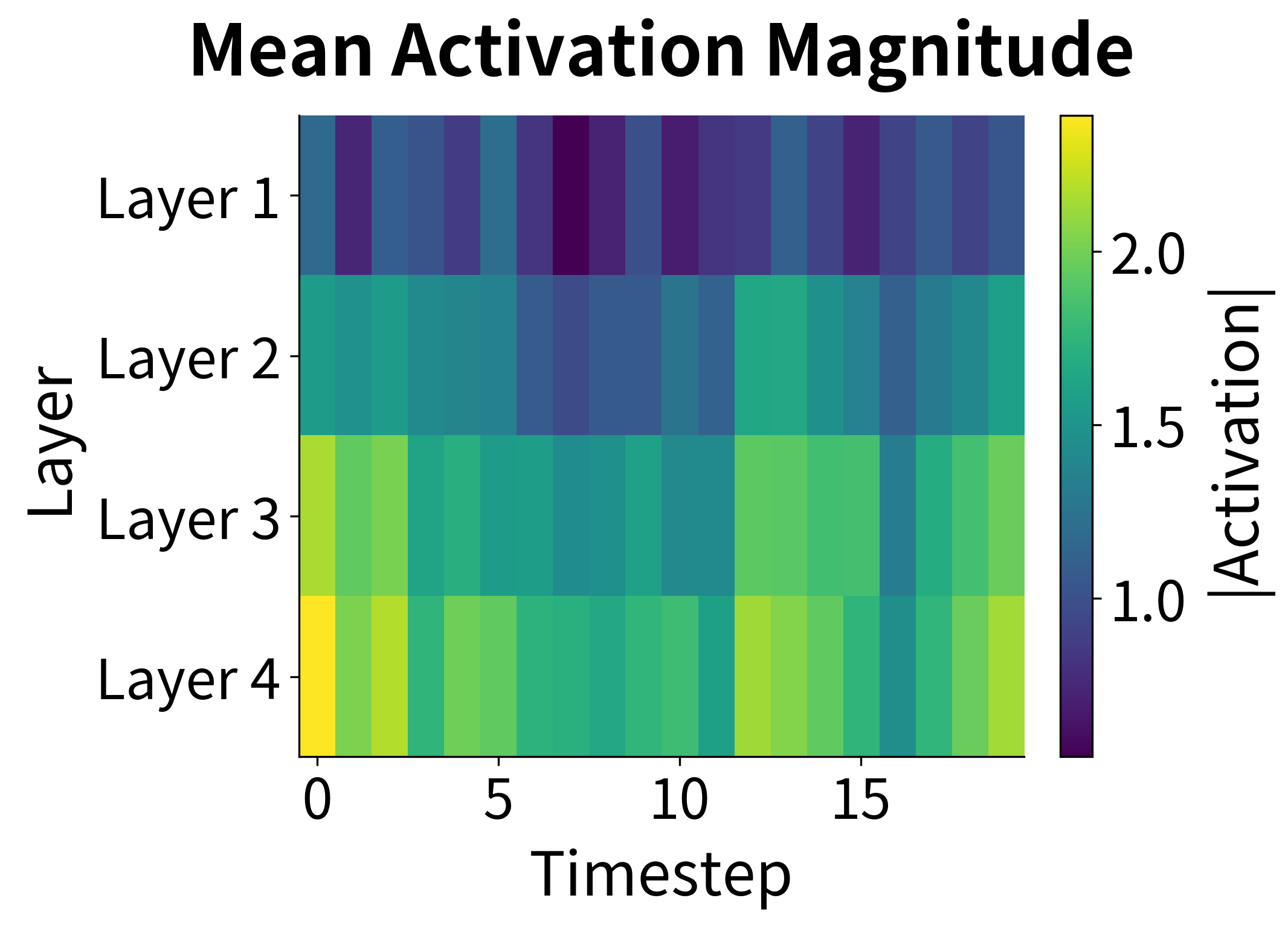
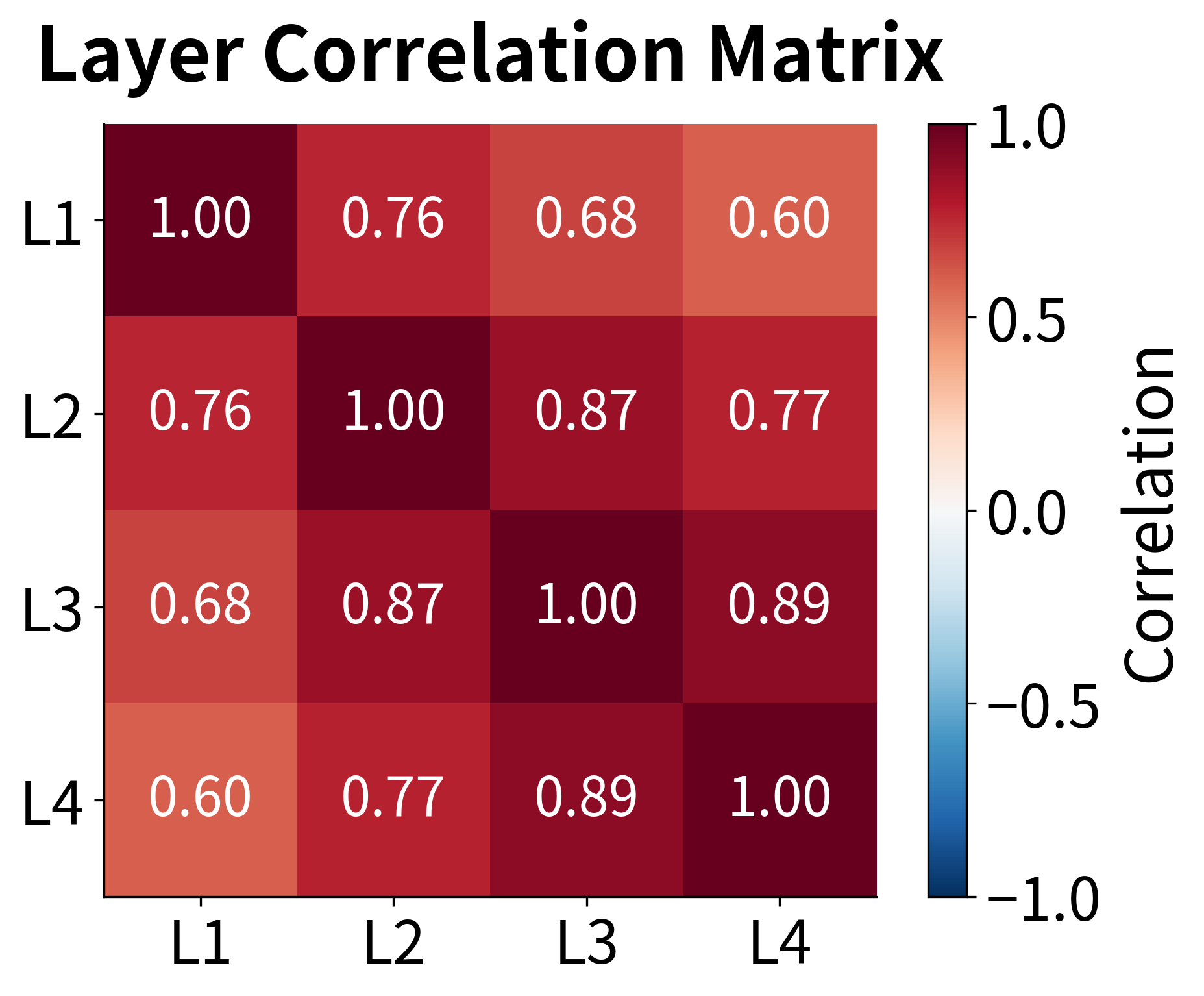
The activation heatmap reveals how information is processed hierarchically. Early layers (1-2) show activation patterns that closely track the input sequence structure, while deeper layers (3-4) develop more distributed, abstract representations. The correlation matrix confirms this: adjacent layers are highly correlated (they share similar information), but the correlation decreases as layers become more separated, indicating that each layer adds unique transformations.
Limitations and Impact
Stacked RNNs represented a significant advance in sequence modeling, enabling the training of deeper networks that could capture more complex hierarchical patterns. However, they come with important limitations that you should understand.
The most fundamental limitation is the sequential nature of RNN computation. Even with multiple layers, you cannot parallelize across timesteps. This means training and inference time scale linearly with sequence length, making stacked RNNs slow for long sequences. A 4-layer stacked LSTM processing a 1000-token sequence must perform 4000 sequential operations, which modern GPUs cannot parallelize effectively.
Memory consumption during training is another practical constraint. Backpropagation through time requires storing all intermediate hidden states and cell states for every layer at every timestep. For a 4-layer LSTM with hidden size 512 processing sequences of length 500, you need to store (for and ) = 2 million float values per sample, plus all the intermediate gate activations. This quickly exhausts GPU memory for large batches or long sequences.
Despite these limitations, stacked RNNs achieved remarkable results and established several important principles. The hierarchical processing paradigm, where lower layers capture local patterns and higher layers capture global structure, influenced subsequent architectures including Transformers. Residual connections and layer normalization, while not invented for RNNs, proved essential for training deep sequence models and became standard components in modern architectures.
The practical sweet spot for stacked RNNs remains 2-6 layers for most applications. Beyond this, the computational overhead outweighs the representational benefits, and you're better served by either wider networks or fundamentally different architectures like Transformers that can parallelize across sequence positions.
Summary
This chapter explored how stacking multiple RNN layers creates deeper networks capable of learning hierarchical representations. We covered the key concepts and techniques that make deep RNNs trainable and effective.
Stacked RNNs pass information both horizontally through time and vertically through layers. Each layer operates on increasingly abstract representations, with the first layer processing raw inputs and subsequent layers processing hidden states from below. This hierarchical structure mirrors the natural hierarchy in many sequential data types, from phonemes to words to sentences in language.
Training deep RNNs requires addressing gradient flow through both temporal and vertical dimensions. Residual connections provide direct gradient pathways that bypass the nonlinear transformations in each layer, dramatically improving gradient flow and enabling training of deeper networks. Layer normalization stabilizes activations across the feature dimension, reducing sensitivity to initialization and enabling larger learning rates.
The practical depth limit for stacked RNNs is typically 4-8 layers. Beyond this, computational overhead increases faster than representational benefits. The choice between depth and width depends on your task: hierarchical data benefits from depth, while tasks requiring rich single-level representations benefit from width.
Key implementation details include:
- Use
num_layersparameter in PyTorch for simple stacking - Add residual connections for networks deeper than 2-3 layers
- Apply layer normalization to stabilize training
- Use dropout between layers (0.1-0.3) for regularization
- Consider bidirectional processing when future context is available
In the next part of this book, we'll explore sequence-to-sequence models that use stacked encoder and decoder networks for tasks like machine translation, where the full power of deep RNNs becomes apparent.
Key Parameters
When building stacked RNNs with PyTorch's nn.LSTM or nn.GRU, these parameters have the most significant impact on model behavior:
-
num_layers: Number of stacked recurrent layers. Start with 2-3 layers for most tasks. Increase to 4-6 for complex sequence-to-sequence problems like machine translation. Beyond 6-8 layers rarely helps and can hurt training stability.
-
hidden_size: Dimensionality of the hidden state at each layer. Larger values (256-1024) provide more capacity but increase computation quadratically. For residual connections, all layers typically use the same hidden size.
-
dropout: Probability of dropping connections between layers (only active when
num_layers > 1). Values of 0.1-0.3 help prevent overfitting. Applied between layers but not within recurrent connections. -
bidirectional: When
True, runs separate forward and backward RNNs and concatenates their outputs, doubling the effective hidden size. Useful for tasks where future context matters (classification, tagging) but not applicable for generation tasks. -
batch_first: When
True, input tensors have shape(batch, seq_len, features). WhenFalse(default), shape is(seq_len, batch, features). Usingbatch_first=Truealigns with common data loading patterns.
For custom implementations with residual connections and layer normalization:
-
residual_projection: Required when input and output dimensions differ (e.g., first layer of bidirectional network). Use
nn.Linearto project the skip connection to match dimensions. -
layer_norm_eps: Epsilon value for layer normalization numerical stability. Default of works well in most cases. Increase if you observe NaN values during training.
Quiz
Ready to test your understanding? Take this quick quiz to reinforce what you've learned about stacked RNNs and deep recurrent networks.

Comments