Vanishing Gradients in RNNs: Why Neural Networks Forget Long Sequences

Recurrent neural networks promise to model sequences of arbitrary length by sharing parameters across time. In theory, an RNN can learn dependencies between the first word of a sentence and the last, no matter how far apart they are. In practice, this promise often breaks down. The culprit? The vanishing gradient problem.

When you train an RNN using backpropagation through time, gradients flow backward from the loss at the final timestep all the way to the earliest inputs. At each step backward, the gradient gets multiplied by the same weight matrix. If the largest eigenvalue of this matrix is less than 1, these repeated multiplications cause the gradient to shrink exponentially. By the time the gradient reaches early timesteps, it has essentially vanished, carrying no useful learning signal.

This chapter dissects the vanishing gradient problem in depth. We'll derive exactly why gradients decay exponentially, visualize this decay, and demonstrate how it prevents RNNs from learning long-range dependencies. We'll also examine the flip side, exploding gradients, and survey the architectural solutions that address these fundamental limitations.

To understand why gradients vanish, we need to trace exactly how learning signals flow through an RNN during training. The story begins with a simple question: when we compute a loss at the end of a sequence, how does that error signal reach the weights that processed the very first input?

The answer involves a chain of multiplications, and this chain structure is precisely what causes the vanishing gradient problem. Let's build up to this insight step by step, starting with the basic RNN computation and then deriving exactly how gradients propagate backward.

Before diving into gradients, let's establish the forward computation. An RNN processes a sequence by maintaining a hidden state that gets updated at each timestep. This update combines three things: the previous hidden state (memory of what came before), the current input (new information), and learned weights (how to combine them).

The standard RNN computes hidden states using the recurrence:

where:

• $\mathbf{h}_t \in \mathbb{R}^d$: the hidden state at timestep $t$, a $d$-dimensional vector encoding what the network "remembers"
• $\mathbf{W}_{hh} \in \mathbb{R}^{d \times d}$: the recurrent weight matrix that transforms the previous hidden state
• $\mathbf{W}_{xh} \in \mathbb{R}^{d \times n}$: the input weight matrix that transforms the current input
• $\mathbf{x}_t \in \mathbb{R}^n$: the input at timestep $t$
• $\mathbf{b}_h \in \mathbb{R}^d$: the bias vector

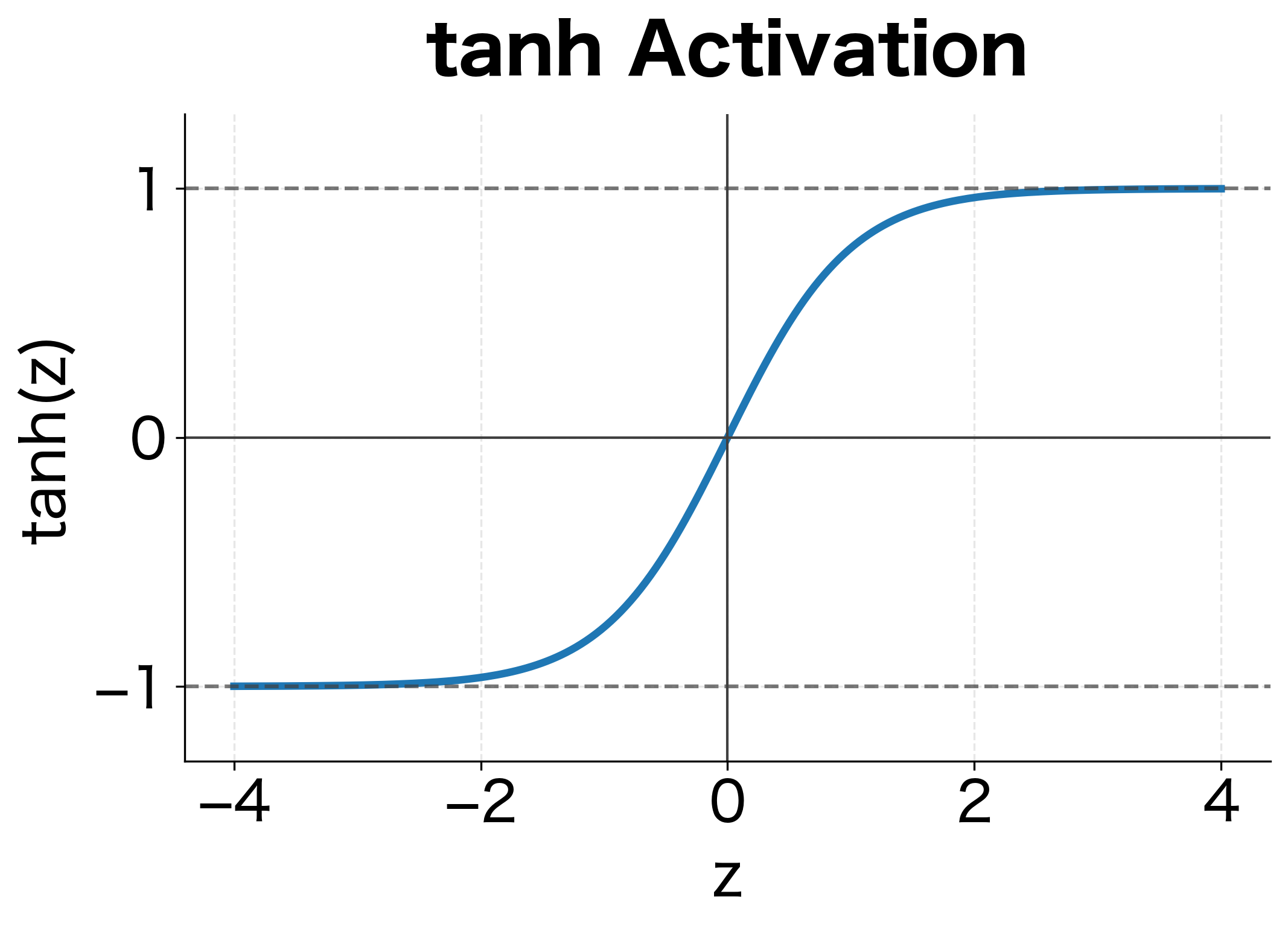
The tanh activation squashes the output to the range $(-1, 1)$, preventing hidden states from growing unboundedly. But as we'll see, this squashing has consequences for gradient flow.

The crucial observation is the recursive dependency: $\mathbf{h}_t$ depends on $\mathbf{h}_{t-1}$, which depends on $\mathbf{h}_{t-2}$, and so on, all the way back to $\mathbf{h}_0$. This means the hidden state at any timestep implicitly depends on all previous inputs and all applications of the weight matrices. When we want to compute how the loss depends on early hidden states, we must trace through this entire chain.

Now we arrive at the heart of the matter: how do gradients flow backward through this recursive structure?

Suppose we compute a loss $\mathcal{L}$ at the final timestep $T$. To update the recurrent weights $\mathbf{W}_{hh}$ using gradient descent, we need $\frac{\partial \mathcal{L}}{\partial \mathbf{W}_{hh}}$, which tells us how to adjust each weight to reduce the loss. But here's the complication: the same weight matrix $\mathbf{W}_{hh}$ is used at every timestep. A small change to $\mathbf{W}_{hh}$ affects $\mathbf{h}_1$, which affects $\mathbf{h}_2$, which affects $\mathbf{h}_3$, and so on. The total effect on the loss accumulates contributions from all these pathways.

Using the chain rule, we can express this accumulated gradient as:

where:

• $\frac{\partial \mathcal{L}}{\partial \mathbf{W}_{hh}}$: the gradient of the loss with respect to the recurrent weight matrix
• $\sum_{t=1}^{T}$: summation over all timesteps, because $\mathbf{W}_{hh}$ influences every hidden state
• $\frac{\partial \mathcal{L}}{\partial \mathbf{h}_T}$: how the loss changes with the final hidden state (computed directly from the loss function)
• $\frac{\partial \mathbf{h}_T}{\partial \mathbf{h}_t}$: how the final hidden state depends on an earlier hidden state at time $t$
• $\frac{\partial \mathbf{h}_t}{\partial \mathbf{W}_{hh}}$: how the hidden state at time $t$ depends directly on the weights

Let's focus on the critical term: $\frac{\partial \mathbf{h}_T}{\partial \mathbf{h}_t}$. This measures how sensitive the final hidden state is to changes in an earlier hidden state. If this term is small, then even if the loss is very sensitive to $\mathbf{h}_T$, that sensitivity won't propagate back to influence how we update weights that affected $\mathbf{h}_t$.

Because each hidden state depends on the previous one through the recurrence ($\mathbf{h}_k$ depends on $\mathbf{h}_{k-1}$), we must chain together all the intermediate derivatives. This is where the product structure emerges. By the chain rule:

where:

• $\prod_{k=t+1}^{T}$: a product of $T - t$ terms, one for each timestep between $t$ and $T$
• $\frac{\partial \mathbf{h}_k}{\partial \mathbf{h}_{k-1}}$: the Jacobian matrix describing how hidden state $k$ depends on hidden state $k-1$

This product structure is the heart of the vanishing gradient problem. To go from timestep $t$ to timestep $T$, we multiply together $T - t$ matrices. If each matrix shrinks vectors (has norm less than 1), the product shrinks exponentially. If each matrix expands vectors (has norm greater than 1), the product explodes exponentially.

To understand what these Jacobian matrices look like, we differentiate the recurrence equation. Starting from $\mathbf{h}_k = \tanh(\mathbf{W}_{hh} \mathbf{h}_{k-1} + \mathbf{W}_{xh} \mathbf{x}_k + \mathbf{b}_h)$, we apply the chain rule to find how $\mathbf{h}_k$ changes when we perturb $\mathbf{h}_{k-1}$:

where:

• $\mathbf{z}_k = \mathbf{W}_{hh} \mathbf{h}_{k-1} + \mathbf{W}_{xh} \mathbf{x}_k + \mathbf{b}_h$: the pre-activation (input to tanh) at timestep $k$
• $\text{diag}(\tanh'(\mathbf{z}_k))$: a $d \times d$ diagonal matrix where entry $(i, i)$ equals $\tanh'(z_k^{(i)})$, the derivative of tanh evaluated at the $i$-th component of $\mathbf{z}_k$
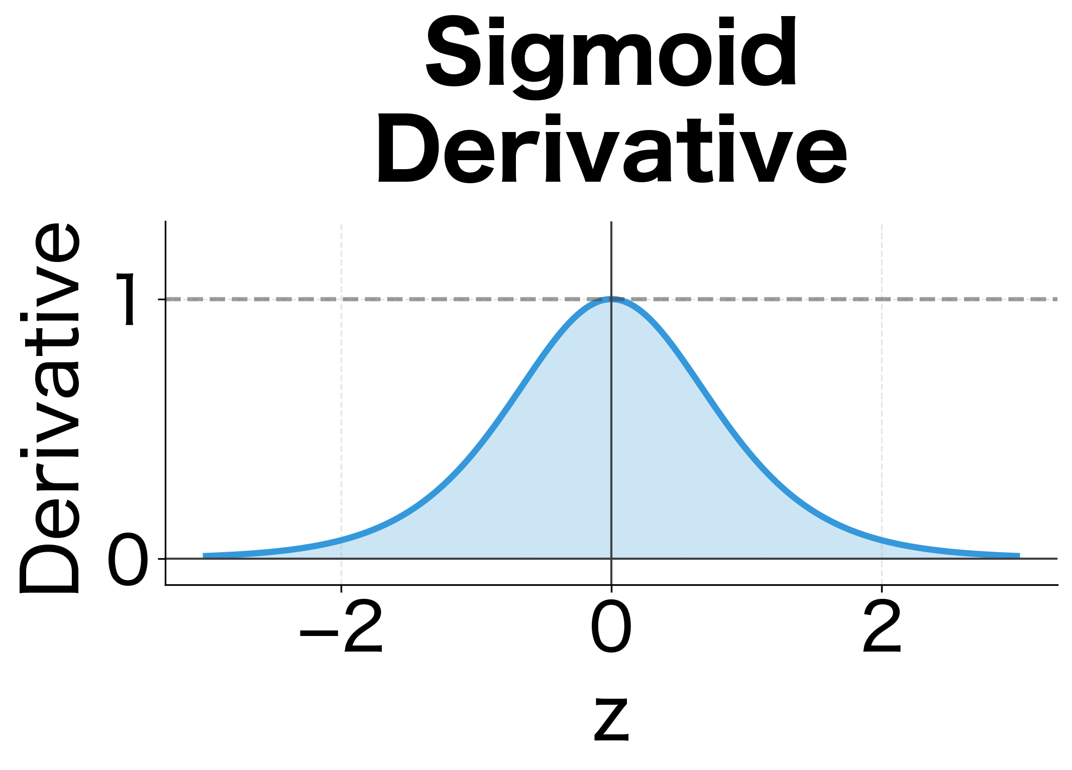
• $\tanh'(z) = 1 - \tanh^2(z)$: the derivative of the tanh function, which is always between 0 and 1
• $\mathbf{W}_{hh}$: the recurrent weight matrix

The Jacobian factors into two components:

1. The diagonal matrix $\text{diag}(\tanh'(\mathbf{z}_k))$: This captures how the tanh activation attenuates the gradient. Since $\tanh'(z) \leq 1$ everywhere, this matrix can only shrink gradients, never amplify them.

2. The weight matrix $\mathbf{W}_{hh}$: This determines how hidden state dimensions mix. Its eigenvalues control whether the overall transformation shrinks or expands vectors.

Now we can write the complete expression for how gradients flow from timestep $T$ back to timestep $t$:

This is a product of $T - t$ matrices, where each matrix is approximately $d \times d$ (the hidden state dimension). The behavior of this product determines whether gradients vanish, explode, or remain stable. If we're computing the gradient for a timestep 50 steps back, we multiply 50 matrices together. Small changes in the magnitude of each factor compound exponentially across these multiplications.

We've established that gradients flow backward through a product of Jacobian matrices. Now let's understand precisely when and why this product shrinks to near-zero.

The key insight comes from linear algebra: when you multiply matrices repeatedly, the behavior of the product is governed by the eigenvalues of those matrices. Eigenvalues tell us how much a matrix stretches or shrinks vectors in different directions. If all eigenvalues have magnitude less than 1, repeated multiplication shrinks any vector toward zero.

To build intuition, consider a simplified case where the tanh derivative is constant (say, close to 1) and we're repeatedly multiplying by $\mathbf{W}_{hh}$. The spectral radius $\rho(\mathbf{W}_{hh})$ is the largest eigenvalue in absolute value, denoted $|\lambda_{\max}|$. This single number largely determines the fate of our gradients.

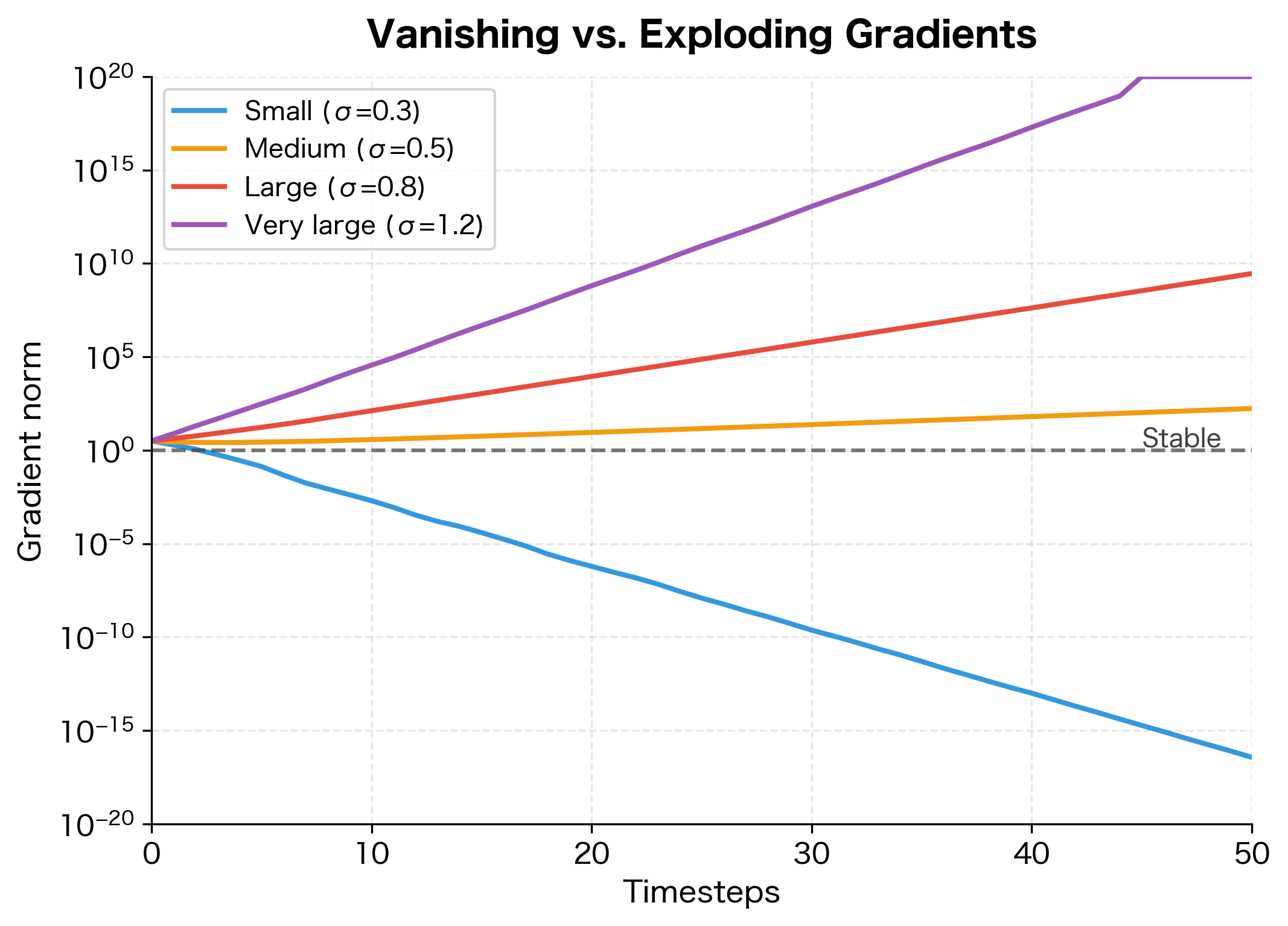
After $n$ multiplications by $\mathbf{W}_{hh}$:

• If $|\lambda_{\max}| < 1$: the product $\mathbf{W}_{hh}^n \to \mathbf{0}$ as $n \to \infty$
• If $|\lambda_{\max}| > 1$: the product $\mathbf{W}_{hh}^n \to \infty$ as $n \to \infty$
• If $|\lambda_{\max}| = 1$: the product may remain bounded

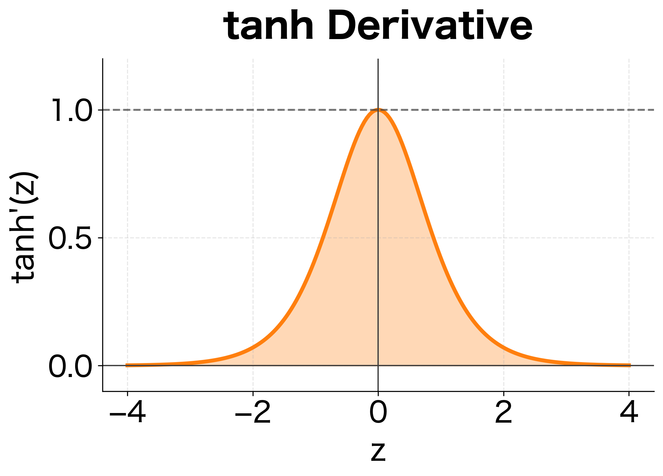
But we can't ignore the tanh derivative. The derivative $\tanh'(z) = 1 - \tanh^2(z)$ has a crucial property: it's always between 0 and 1, with equality to 1 only when $z = 0$. In practice, hidden state values are rarely exactly zero, so the derivative is typically around 0.5 or less. When activations saturate (large positive or negative values), the derivative approaches 0.

This means the diagonal matrix $\text{diag}(\tanh'(\mathbf{z}_k))$ acts as an additional shrinking factor at every timestep. Even if $\mathbf{W}_{hh}$ has spectral radius close to 1, the tanh derivative pulls the effective decay factor below 1.

To see what typical tanh derivative values look like in practice, let's simulate an RNN and collect the pre-activation values:

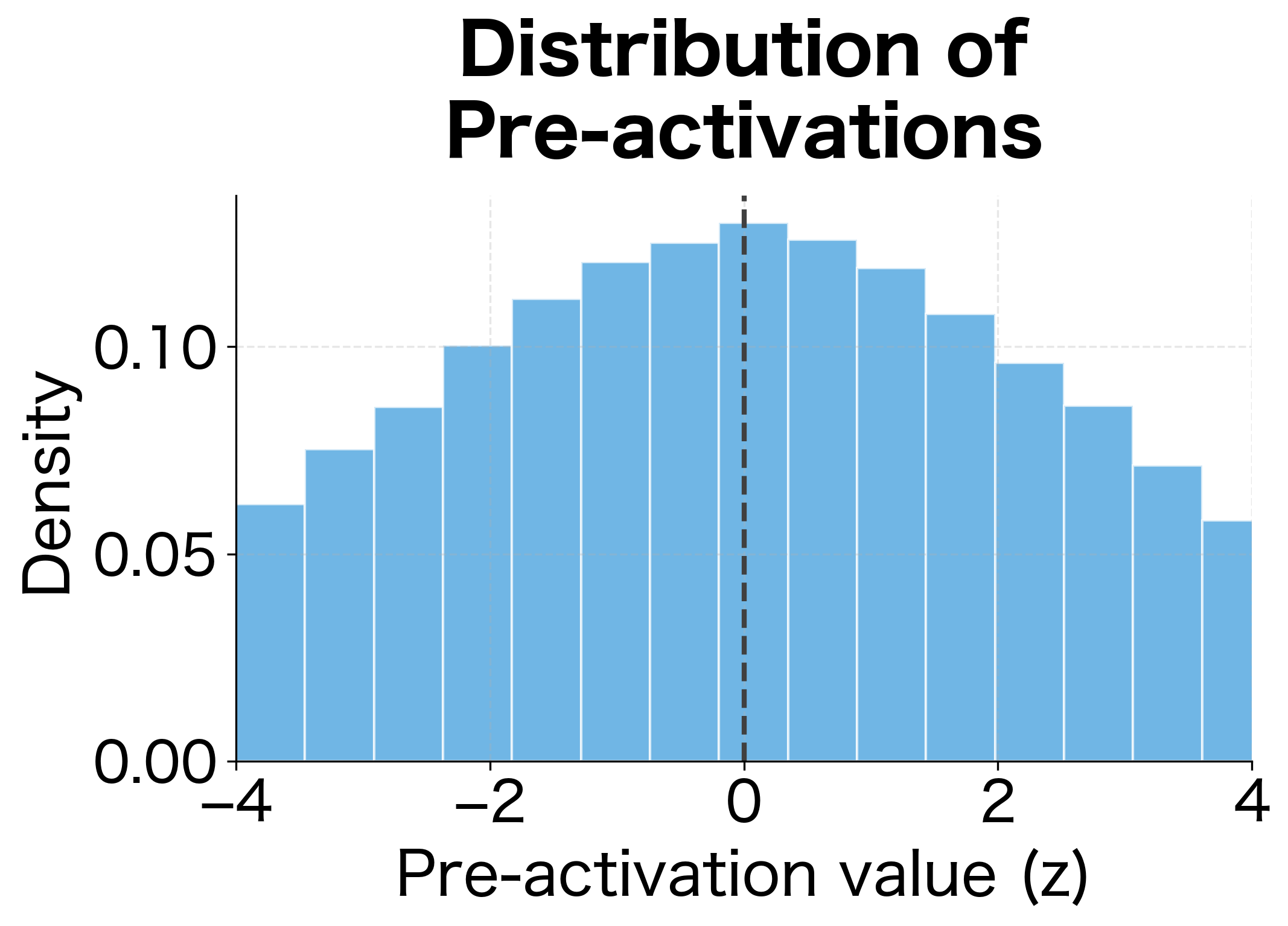
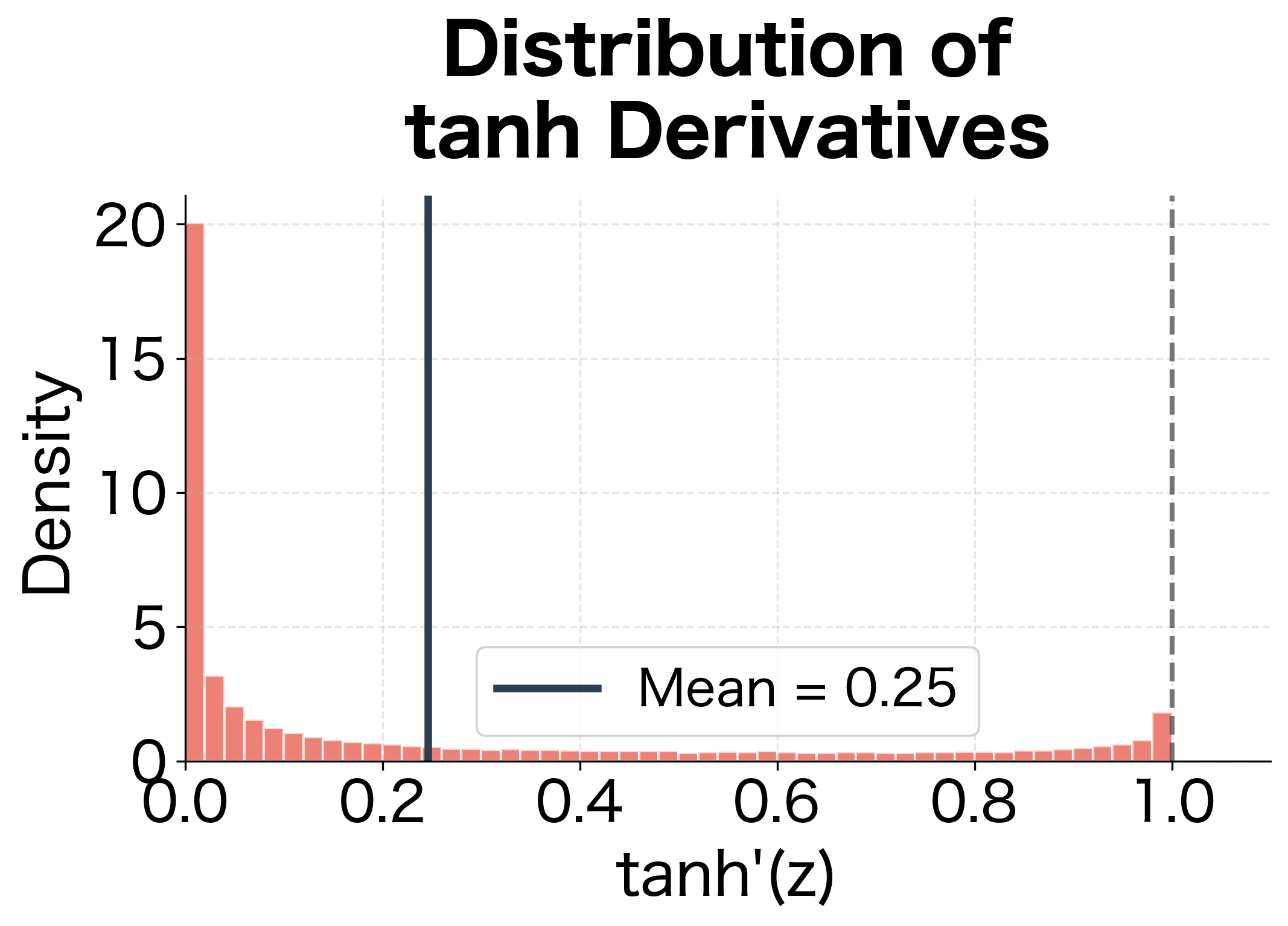
The simulation reveals why gradients vanish: even though tanh derivatives can reach 1, they rarely do in practice. The mean derivative is around 0.6, meaning each timestep shrinks gradients by roughly 40%. Combined with the weight matrix's contribution, the effective decay factor is typically well below 1.

Let's put concrete numbers to this analysis. We can approximate the gradient magnitude by considering the "effective decay factor" at each timestep. This factor combines the contribution from the weight matrix eigenvalues and the tanh derivative.

Suppose the tanh derivative averages 0.5 across timesteps (a reasonable estimate for non-saturated activations), and suppose the spectral radius of $\mathbf{W}_{hh}$ is 0.9. The gradient magnitude after $n$ backward steps scales roughly as:

where:

• $\|\text{gradient}\|$: the magnitude (norm) of the gradient vector
• $\gamma$: the effective decay factor per timestep, approximately $\gamma \approx \bar{\sigma} \cdot |\lambda_{\max}|$
• $\bar{\sigma}$: the average tanh derivative (here $\bar{\sigma} \approx 0.5$)
• $|\lambda_{\max}|$: the spectral radius of $\mathbf{W}_{hh}$ (here $|\lambda_{\max}| = 0.9$)
• $n$: the number of timesteps the gradient must travel backward

With our example values, $\gamma = 0.5 \times 0.9 = 0.45$, so:

After just 10 timesteps, this factor is $0.45^{10} \approx 0.00034$, meaning the gradient has shrunk by a factor of nearly 3,000. After 20 timesteps, it's $0.45^{20} \approx 10^{-7}$. The gradient has essentially vanished into numerical noise.

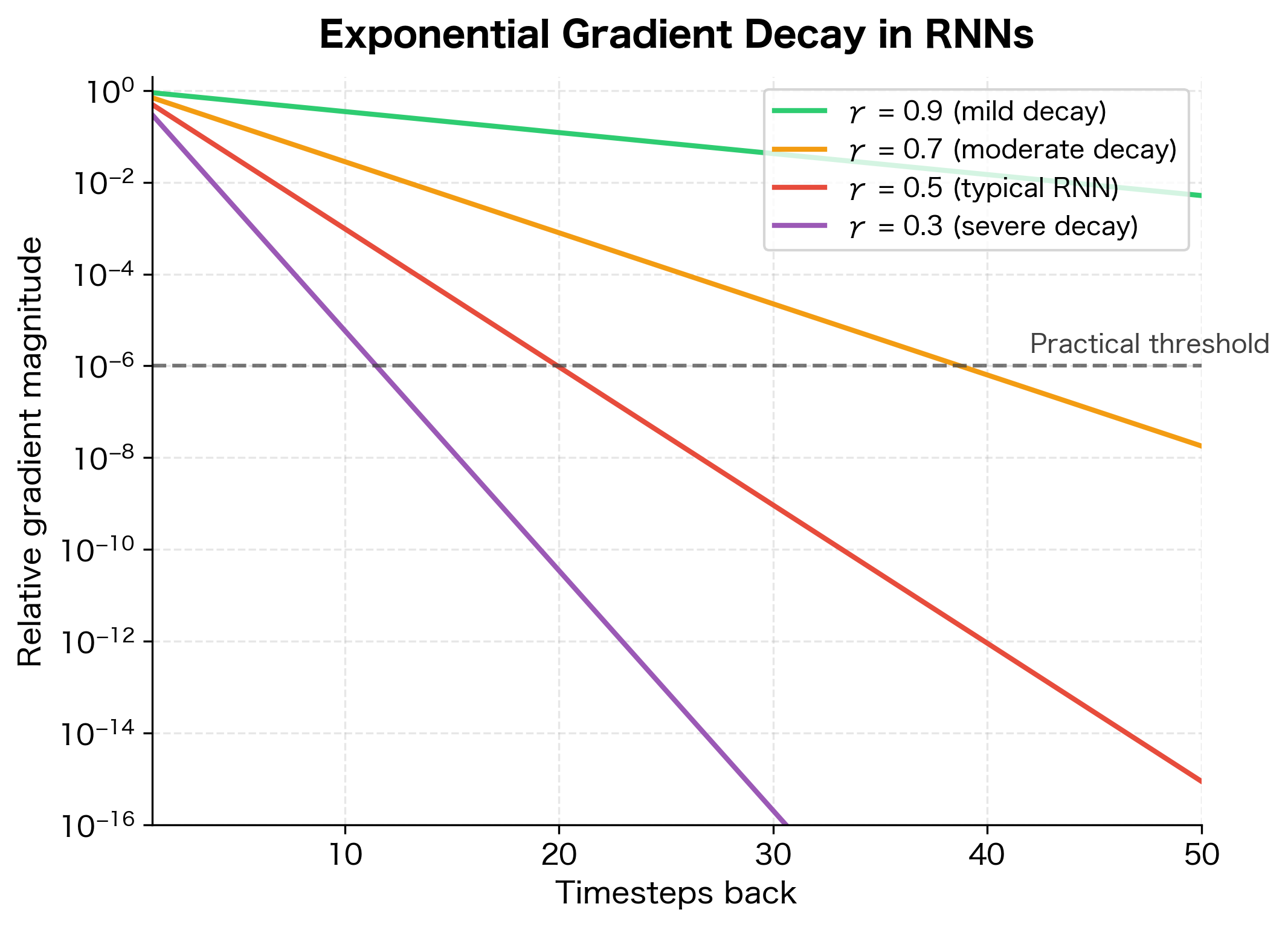
This exponential decay is the core of the vanishing gradient problem. Information from early timesteps cannot effectively influence the weight updates because the gradient signal decays to numerical insignificance before reaching them.

Let's build a simple RNN and observe gradient flow directly. We'll create a sequence prediction task and measure how gradients decay as they propagate backward through time.

This RNN stores all hidden states so we can examine gradients at each timestep. Let's create a simple task and measure gradient magnitudes.

Now we can examine how gradients flow to each hidden state. We'll use PyTorch hooks to capture gradient magnitudes at each timestep.

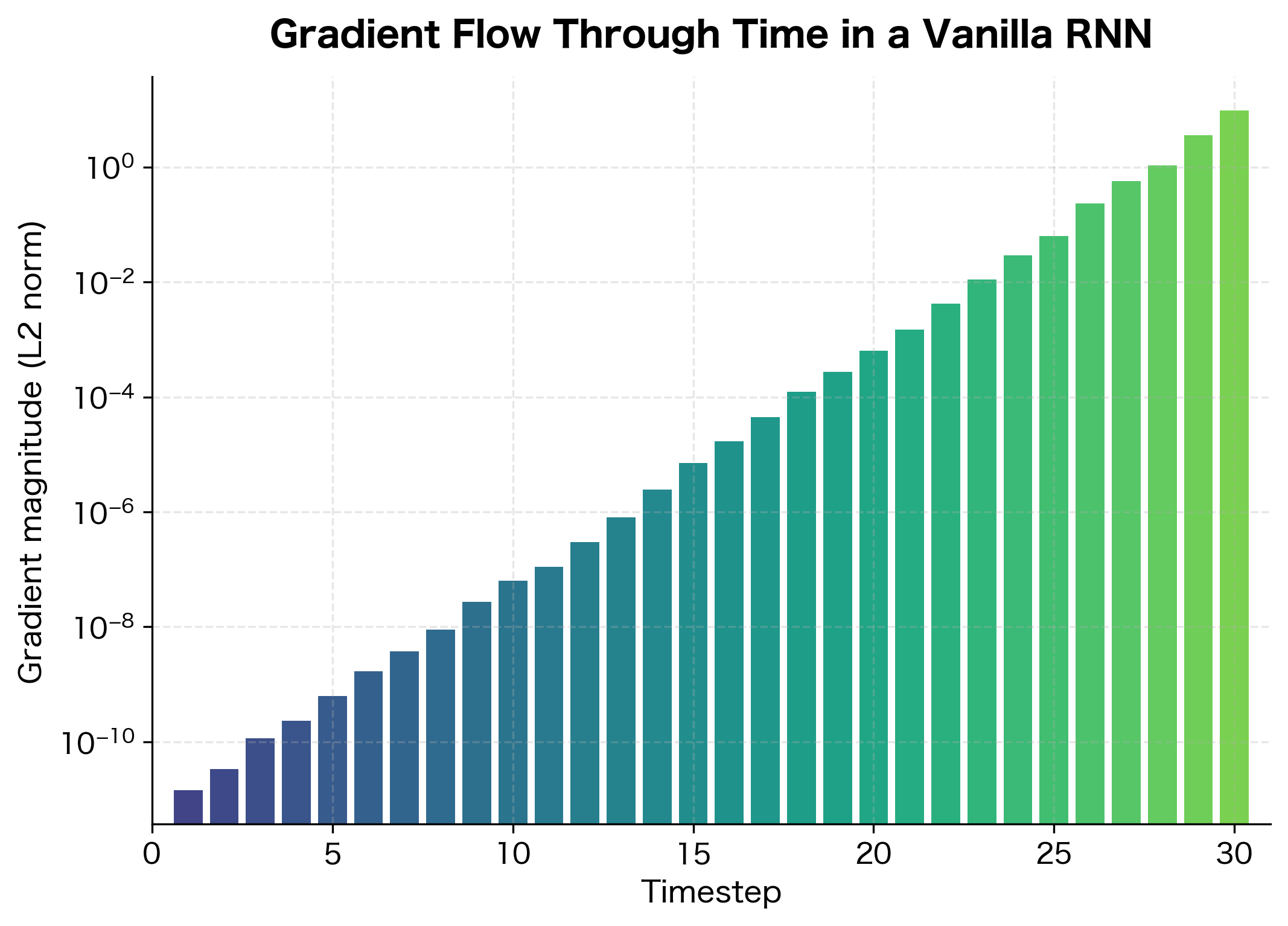
The visualization reveals the problem starkly. Gradients at the final timesteps are orders of magnitude larger than those at early timesteps. Any information about how early inputs should influence the output is washed away by this exponential decay.

The vanishing gradient problem isn't just a mathematical curiosity. It has direct consequences for what RNNs can learn. Let's construct a task that explicitly requires long-range dependencies and watch a vanilla RNN struggle.

A classic benchmark for long-range dependencies is the copying task. The network sees a sequence of random symbols, followed by a delay period of blank symbols, then must reproduce the original sequence. Success requires remembering information across the entire delay.

The input sequence shows random symbols (1-8) at the beginning, followed by zeros (blanks) during the delay period, then a marker (9), and finally more blanks where the network should output its predictions. The target is all zeros except at the very end, where it contains the original symbols the network must recall. This task is particularly challenging because the gradient signal from the recall phase must travel backward through 20+ timesteps of blanks to reach the encoding phase.

Let's train a vanilla RNN on this task and observe its failure to learn long-range dependencies.

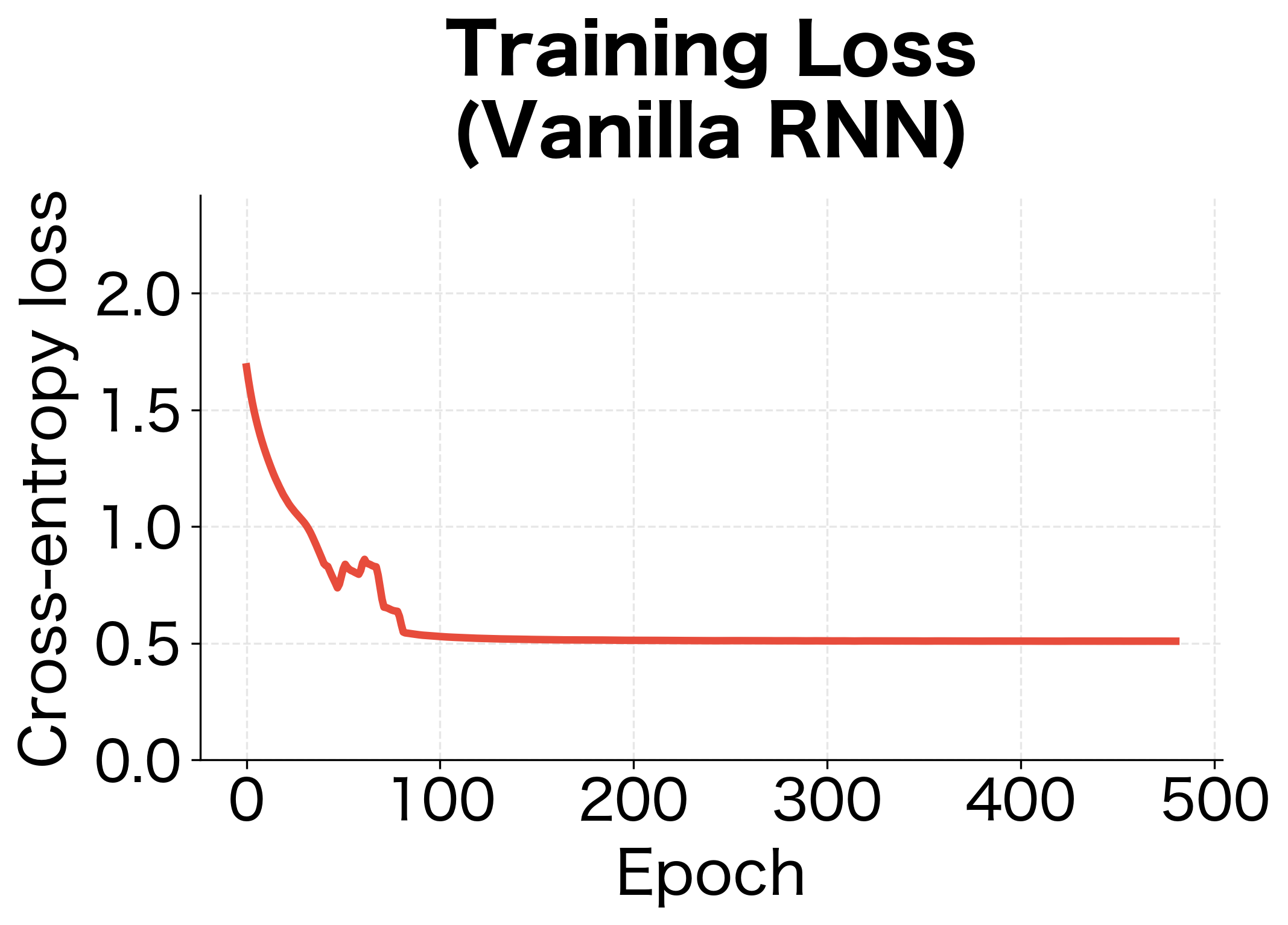
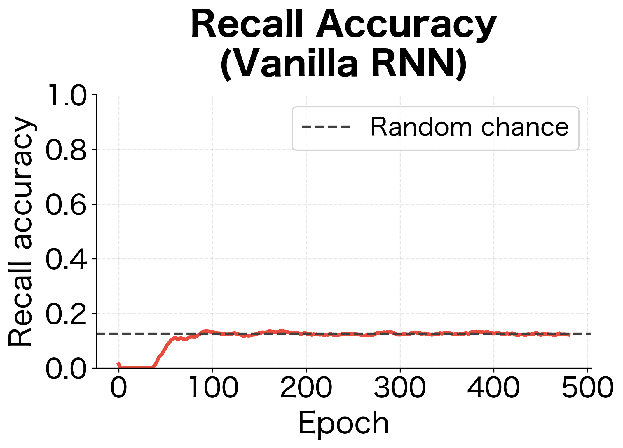
The vanilla RNN fails to learn the copying task. Its recall accuracy hovers near random chance because gradients from the output phase cannot effectively propagate back through 20+ timesteps to inform how the network should encode the original symbols.

We've focused on vanishing gradients, but the same mathematical machinery can cause the opposite problem: exploding gradients. When the spectral radius of the Jacobian exceeds 1, gradients grow exponentially instead of shrinking.

The same analysis that explains vanishing gradients also predicts when gradients will explode. If the effective decay factor exceeds 1, gradients grow instead of shrink. Specifically, if $|\lambda_{\max}| > 1$ (and the tanh derivatives don't shrink the gradients enough to compensate), the gradient product explodes:

where:

• $\left\| \cdot \right\|$: the matrix norm (measuring the "size" of the gradient)
• $\prod_{k=t+1}^{T}$: the product of Jacobian matrices from timestep $t+1$ to $T$
• $T - t$: the number of timesteps the gradient travels backward

As the sequence length increases, this product grows without bound. Exploding gradients manifest as:

• NaN or Inf values during training
• Extremely large weight updates that destabilize learning
• Loss values that spike unpredictably

Here's a crucial insight: vanishing and exploding gradients are not symmetric problems. Exploding gradients can be mitigated with gradient clipping, a simple technique that rescales gradients when their norm exceeds a threshold:

The original gradient had a norm of approximately 1000 (100 elements each scaled by 100), but after clipping it's reduced to exactly 1.0. The gradient direction is preserved, only the magnitude is scaled down. This prevents the catastrophically large weight updates that would otherwise destabilize training.

Gradient clipping is standard practice in RNN training. However, there is no analogous fix for vanishing gradients. You cannot amplify a gradient that has already decayed to zero, because you've lost the information about which direction to go. This asymmetry is why vanishing gradients are the more fundamental problem.

The vanishing gradient problem reveals a fundamental tension in RNN design. To learn long-range dependencies, gradients must flow across many timesteps without decaying. But the repeated multiplication inherent in backpropagation through time makes stable gradient flow mathematically difficult.

You might wonder: can't we just initialize weights carefully or use different activation functions? Let's examine why these approaches fall short.

Careful initialization: We could initialize $\mathbf{W}_{hh}$ as an orthogonal matrix (eigenvalues with magnitude 1). This helps initially, but as training progresses, the weights change and typically lose their orthogonality. The gradient problem resurfaces.

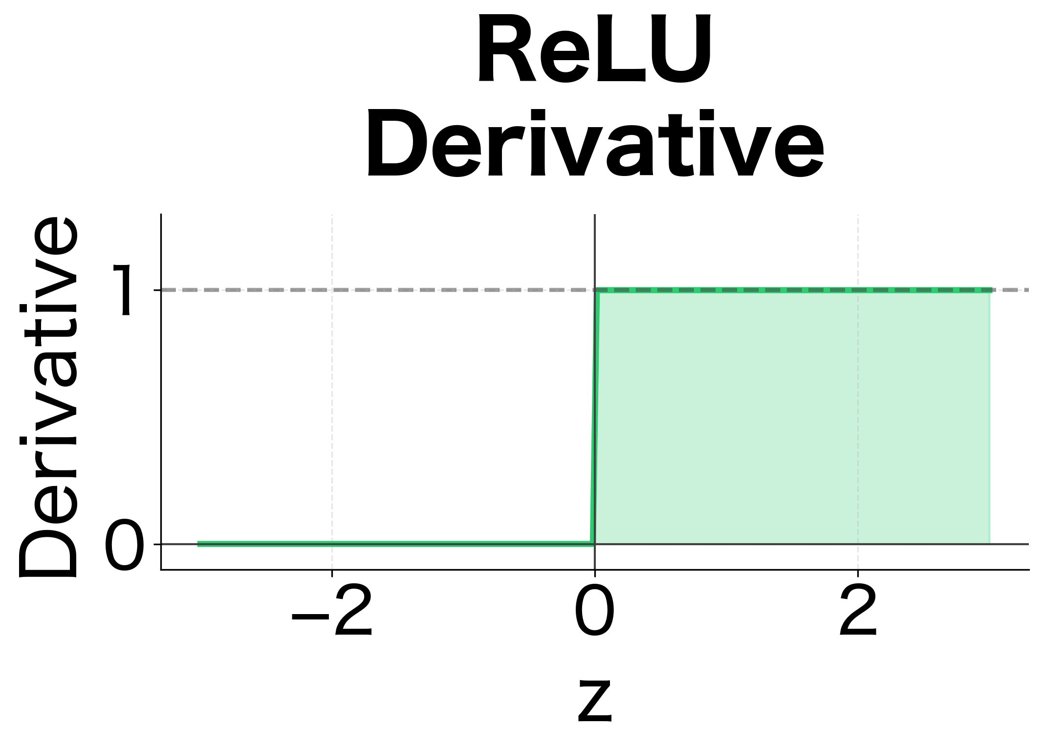
ReLU activation: Unlike tanh, ReLU has derivative 1 for positive inputs. But ReLU creates a different problem: hidden states can grow unboundedly since there's no squashing. The network becomes unstable.

Smaller learning rates: This slows down training but doesn't address the fundamental issue. Gradients still vanish; we just take smaller steps in directions that are already nearly zero.

The vanishing gradient problem cannot be solved by tweaking hyperparameters or initialization schemes. It requires a fundamental change in how information flows through the network. The solution is to create alternative paths for gradient flow that bypass the problematic repeated multiplications.

This insight led to the development of gated architectures:

• LSTM (Long Short-Term Memory): Introduces a cell state that acts as a "gradient highway," allowing information to flow across many timesteps with minimal transformation.
• GRU (Gated Recurrent Unit): A simplified gating mechanism that achieves similar benefits with fewer parameters.

These architectures don't eliminate the Jacobian products entirely. Instead, they introduce additive connections that allow gradients to flow without repeated multiplication. We'll explore these solutions in detail in the following chapters.

The mathematical analysis above tells us that gradients should decay exponentially. But how does this play out in practice with actual numbers? Let's trace through a complete example, computing every intermediate value by hand, to see the vanishing gradient problem unfold step by step.

This worked example serves two purposes: it grounds the abstract formulas in concrete computation, and it reveals the quantitative severity of the problem even for very short sequences.

We'll use the simplest possible RNN: hidden size $d = 2$ (so we can easily visualize the matrices) and a simplified recurrence that ignores inputs:

where:

• $\mathbf{h}_t \in \mathbb{R}^2$: the hidden state vector at timestep $t$
• $\mathbf{W}_{hh} \in \mathbb{R}^{2 \times 2}$: the recurrent weight matrix
• $\tanh$: applied elementwise to the vector

We use a specific weight matrix with moderate values:

Let's verify our expectation about this matrix. The eigenvalues of $\mathbf{W}_{hh}$ are approximately 0.45 + 0.087i and 0.45 - 0.087i, both with magnitude around 0.46. Since $|\lambda_{\max}| < 1$, we expect gradients to decay. Combined with the tanh derivative (which further shrinks gradients), the decay should be substantial even over just 5 timesteps.

Starting from the initial hidden state $\mathbf{h}_0 = (1, 0)^T$, we'll trace through two phases:

1. Forward pass: Compute $\mathbf{h}_1, \mathbf{h}_2, \ldots, \mathbf{h}_5$ and the pre-activations $\mathbf{z}_1, \ldots, \mathbf{z}_5$
2. Backward pass: Compute the Jacobians at each timestep and multiply them to find $\frac{\partial \mathbf{h}_5}{\partial \mathbf{h}_0}$

The forward pass shows how the hidden state evolves over time. Starting from $\mathbf{h}_0 = (1, 0)$, each timestep applies the weight matrix and then the tanh nonlinearity. Notice how the hidden state values quickly settle into a range where tanh derivatives will be less than 1, setting up the conditions for gradient decay.

Now comes the crucial part: computing how gradients flow backward. We want $\frac{\partial \mathbf{h}_5}{\partial \mathbf{h}_0}$, which tells us how a small perturbation to the initial hidden state affects the final hidden state. By the chain rule, this equals the product of all five intermediate Jacobians:

Each Jacobian has the form $\text{diag}(\tanh'(\mathbf{z}_k)) \cdot \mathbf{W}_{hh}$. Let's compute them:

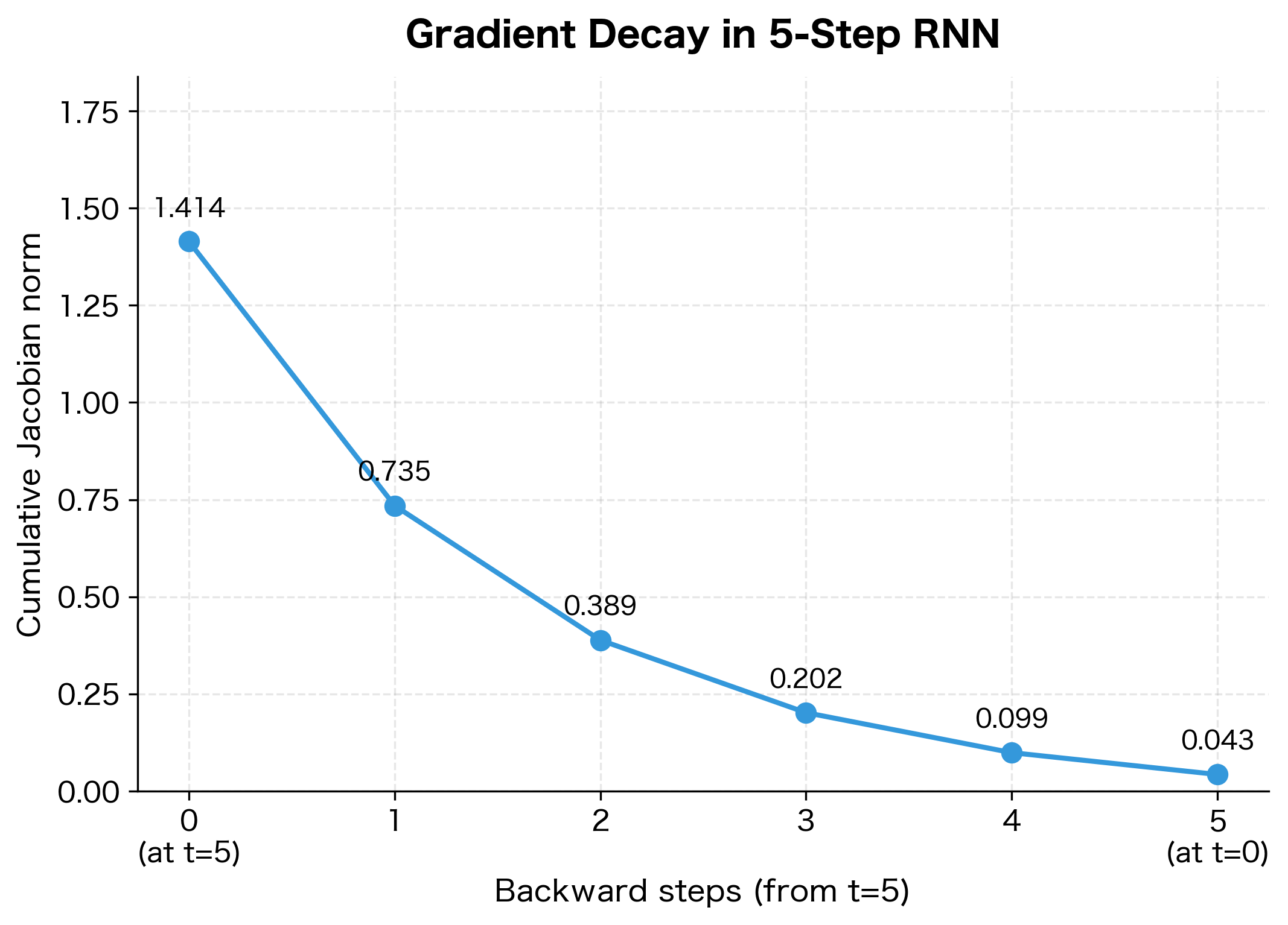
Each Jacobian has a spectral radius well below 1 (around 0.3-0.4), meaning each backward step shrinks the gradient. The total Jacobian, computed by multiplying all five intermediate Jacobians, has a Frobenius norm that's a small fraction of the identity matrix's norm (1.41). This quantifies exactly how much gradient information is lost over just 5 timesteps.

To visualize this decay, let's look at the cumulative Jacobian as we multiply backward through time. We start with the identity matrix (representing "no transformation yet") and progressively multiply by each Jacobian:

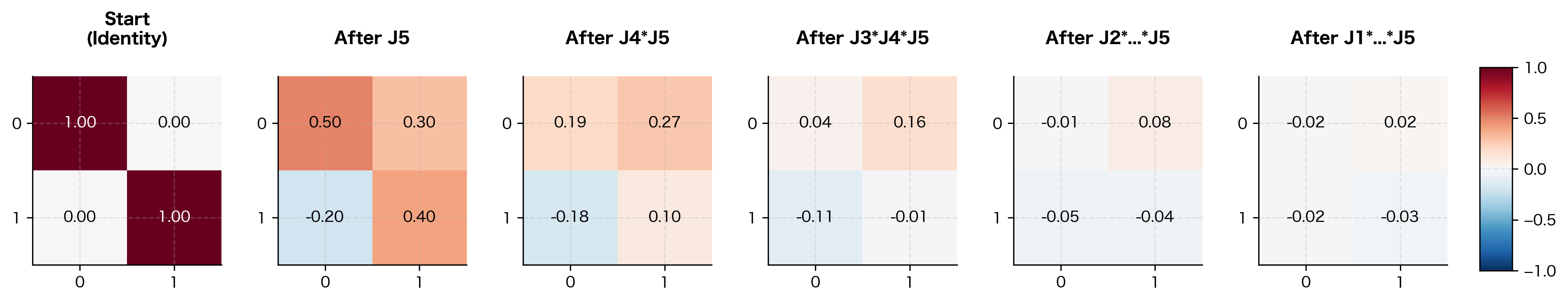
The heatmaps make the decay viscerally clear: the identity matrix starts with 1s on the diagonal, but after just 5 multiplications, all entries have shrunk toward zero. The gradient information has been systematically attenuated at each step.

This worked example crystallizes the vanishing gradient problem:

1. Each Jacobian shrinks: Every intermediate Jacobian has spectral radius well below 1 (around 0.3-0.4), meaning each step backward shrinks the gradient.

2. Decay compounds multiplicatively: The total Jacobian norm after 5 steps is roughly $(0.35)^5 \approx 0.005$, meaning gradients have decayed by a factor of 200.

3. Extrapolation is sobering: For a 50-timestep sequence, the decay factor would be approximately $(0.35)^{50} \approx 10^{-23}$, far below machine precision.

For real-world sequences with hundreds or thousands of timesteps, the decay is catastrophic. This is why vanilla RNNs cannot learn long-range dependencies, no matter how much data or compute you throw at them.

The vanishing gradient problem fundamentally limits what vanilla RNNs can learn. Understanding these limitations clarifies why more sophisticated architectures became necessary.

Vanilla RNNs struggle with tasks requiring dependencies beyond approximately 10-20 timesteps. This includes:

• Language modeling with long context: Predicting the next word often requires understanding sentence structure established many words earlier. A vanilla RNN cannot maintain this context.
• Document classification: Understanding a document's topic requires integrating information across paragraphs. Gradients from the classification loss cannot reach early sentences.
• Time series with long periodicity: Seasonal patterns in data (daily, weekly, yearly cycles) require remembering information across the cycle length.
• Question answering: Answering questions about a passage requires connecting the question to relevant parts of the passage, which may be far apart.

The vanishing gradient problem, first clearly articulated by Hochreiter (1991) and Bengio et al. (1994), motivated a generation of architectural innovations. These researchers showed mathematically why RNNs fail on long sequences and pointed toward solutions involving gating mechanisms.

The LSTM architecture, introduced by Hochreiter and Schmidhuber in 1997, directly addresses vanishing gradients by creating a "cell state" that can carry information across many timesteps without repeated nonlinear transformations. The key insight is additive updates: instead of computing $\mathbf{h}_t = f(\mathbf{W}\mathbf{h}_{t-1})$ where gradients must pass through a nonlinearity at every step, LSTMs compute:

where:

• $\mathbf{c}_t$: the cell state at timestep $t$
• $\mathbf{c}_{t-1}$: the cell state from the previous timestep
• $\Delta\mathbf{c}_t$: the update to the cell state, controlled by learned gates

The addition operation is crucial: when we backpropagate through $\mathbf{c}_t = \mathbf{c}_{t-1} + \Delta\mathbf{c}_t$, the gradient with respect to $\mathbf{c}_{t-1}$ is simply 1 (plus any contribution through $\Delta\mathbf{c}_t$). This creates a "gradient highway" where information can flow backward across many timesteps without multiplicative decay.

This architectural shift enabled RNNs to finally learn long-range dependencies, unlocking applications in machine translation, speech recognition, and text generation that had been impossible with vanilla RNNs. The next chapter explores the LSTM architecture in detail.

The vanishing gradient problem is a fundamental limitation of vanilla RNNs that prevents them from learning long-range dependencies. Here are the key takeaways:

• Gradient chain multiplication: Backpropagation through time computes gradients as products of Jacobian matrices, one for each timestep. When these Jacobians have spectral radius less than 1, gradients shrink exponentially.

• Tanh makes it worse: The tanh activation function has derivative bounded by 1, with typical values around 0.5. This compounds the decay at each timestep.

• Quantitative decay: With typical RNN parameters, gradients decay by factors of $10^3$ to $10^7$ over just 20-30 timesteps, making early inputs effectively invisible to the learning process.

• Asymmetric problem: While exploding gradients can be addressed with gradient clipping, vanishing gradients cannot be recovered because the directional information is lost.

• Architectural solution needed: No amount of hyperparameter tuning can fix the vanishing gradient problem. It requires architectural changes that create alternative gradient pathways, leading to gated architectures like LSTM and GRU.

Understanding the vanishing gradient problem is essential for appreciating why modern sequence models are designed the way they are. The LSTM architecture, which we explore next, directly addresses these limitations by introducing gates that control information flow and a cell state that acts as a gradient highway.

When working with vanilla RNNs and diagnosing gradient flow issues, several parameters significantly impact whether gradients vanish or explode:

• hidden_size: The dimensionality of the hidden state vector. Larger hidden sizes increase model capacity but don't directly solve vanishing gradients. The gradient behavior depends more on the weight matrix eigenvalues than the hidden dimension.

• Weight initialization scale: Controls the spectral radius of $\mathbf{W}_{hh}$. Smaller scales (e.g., gain=0.5 in Xavier initialization) help prevent exploding gradients but accelerate vanishing. Orthogonal initialization can maintain gradient magnitude initially but loses effectiveness as weights change during training.

• nonlinearity: The activation function choice affects gradient flow. Tanh derivatives are bounded by 1 and typically average around 0.5, compounding decay. ReLU has derivative 1 for positive inputs but causes unbounded hidden state growth. Neither solves the fundamental problem in vanilla RNNs.

• Gradient clipping threshold (max_norm): When using torch.nn.utils.clip_grad_norm_, this parameter caps the gradient norm to prevent exploding gradients. Common values range from 1.0 to 5.0. Lower thresholds provide more stability but may slow learning; higher thresholds allow faster updates but risk instability.

• Sequence length: Longer sequences exacerbate vanishing gradients because gradients must travel through more multiplicative steps. For vanilla RNNs, effective gradient flow typically degrades beyond 10-20 timesteps. Tasks requiring longer dependencies need gated architectures like LSTM or GRU.

Ready to test your understanding? Take this quick quiz to reinforce what you've learned about the vanishing gradient problem in recurrent neural networks.