

Master backpropagation from computational graphs to gradient flow. Learn the chain rule, implement forward/backward passes, and understand automatic differentiation.

This article is part of the free-to-read Language AI Handbook
Choose your expertise level to adjust how many terms are explained. Beginners see more tooltips, experts see fewer to maintain reading flow. Hover over underlined terms for instant definitions.
Backpropagation
How does a neural network learn? In the previous chapters, we built multilayer perceptrons that transform inputs through layers of weights and activations, and we defined loss functions that measure prediction quality. But we haven't answered the fundamental question: how do we update the millions of parameters in a neural network to reduce the loss?
The answer is backpropagation, short for "backward propagation of errors." This algorithm computes the gradient of the loss function with respect to every weight in the network, telling us exactly how to adjust each parameter to improve predictions. Backpropagation is arguably the most important algorithm in deep learning. Without it, training neural networks would be computationally intractable.
This chapter builds backpropagation from the ground up. We start with computational graphs that visualize how operations compose, then review the chain rule that makes gradient computation tractable. You'll trace through forward and backward passes step by step, understand gradient accumulation, and implement backpropagation from scratch. By the end, you'll see exactly how modern deep learning frameworks like PyTorch compute gradients automatically.
The Gradient Problem
Neural networks have millions of parameters. GPT-3 has 175 billion. How do we figure out which direction to nudge each one to reduce the loss?
Calculus gives us the answer: the gradient. For a function where is a vector of parameters, the gradient is a vector that points in the direction of steepest increase of . Each component of the gradient tells us how sensitive the function is to changes in the corresponding parameter. To minimize the loss, we move in the opposite direction, the direction of steepest decrease:
where:
- : the updated parameter vector after one step
- : the current parameter vector before the update
- : the learning rate, a small positive scalar (typically 0.001 to 0.1) that controls how large each step is
- : the gradient of the loss with respect to parameters, a vector with the same shape as , where each entry indicates how much the loss would increase if we increased by a tiny amount
- : the loss function, a scalar value measuring prediction error
The subtraction makes intuitive sense: if , increasing would increase the loss, so we decrease it instead. This is gradient descent, simple in concept, but the challenge is computing when the loss depends on parameters through many nested operations.
Consider a 3-layer network. The loss depends on the output, which depends on the third layer's activations, which depend on the second layer's activations, which depend on the first layer's activations, which depend on the input and the first layer's weights. This chain of dependencies seems hopelessly complex to differentiate.
Backpropagation is an algorithm for efficiently computing gradients in neural networks by applying the chain rule systematically from output to input. It computes the gradient of the loss with respect to every parameter in a single backward pass through the network.
Backpropagation solves this problem elegantly. By applying the chain rule in reverse order, from output back to input, we can compute all gradients in time proportional to a single forward pass. This efficiency is what makes training deep networks practical.
Computational Graphs
Before diving into backpropagation, we need a way to visualize how computations flow through a network. A computational graph represents a mathematical expression as a directed graph where nodes are operations and edges show data flow.
Building Blocks of Computation
Every neural network computation breaks down into elementary operations: addition, multiplication, matrix products, and activation functions. A computational graph makes these explicit. Consider the simple expression:
This decomposes into two operations:
- (addition)
- (multiplication)
where:
- : the input variables to the function
- : an intermediate value that stores the result of the first operation
- : the final output of the computation
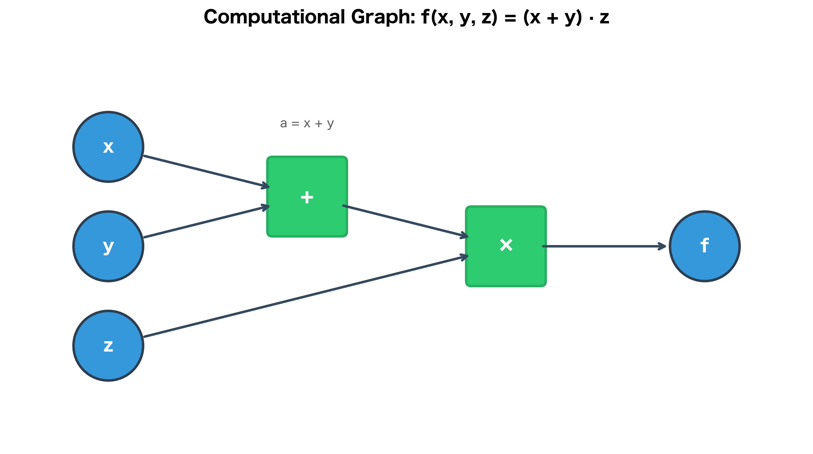
The graph shows data flowing from inputs (x, y, z) through operations (+, ×) to the output (f). The intermediate value is stored at the addition node. This decomposition is the key insight: complex expressions are just chains of simple operations.
Neural Network as a Computational Graph
A neural network layer performs the computation , where:
- : the input vector (or the output from the previous layer)
- : the weight matrix, with shape (output neurons × input neurons)
- : the bias vector, with one value per output neuron
- : the activation function (e.g., ReLU, sigmoid)
- : the output activations
Let's break this into its constituent operations:
- (matrix multiplication: transforms input through learned weights)
- (bias addition: shifts the output)
- (activation: introduces nonlinearity)
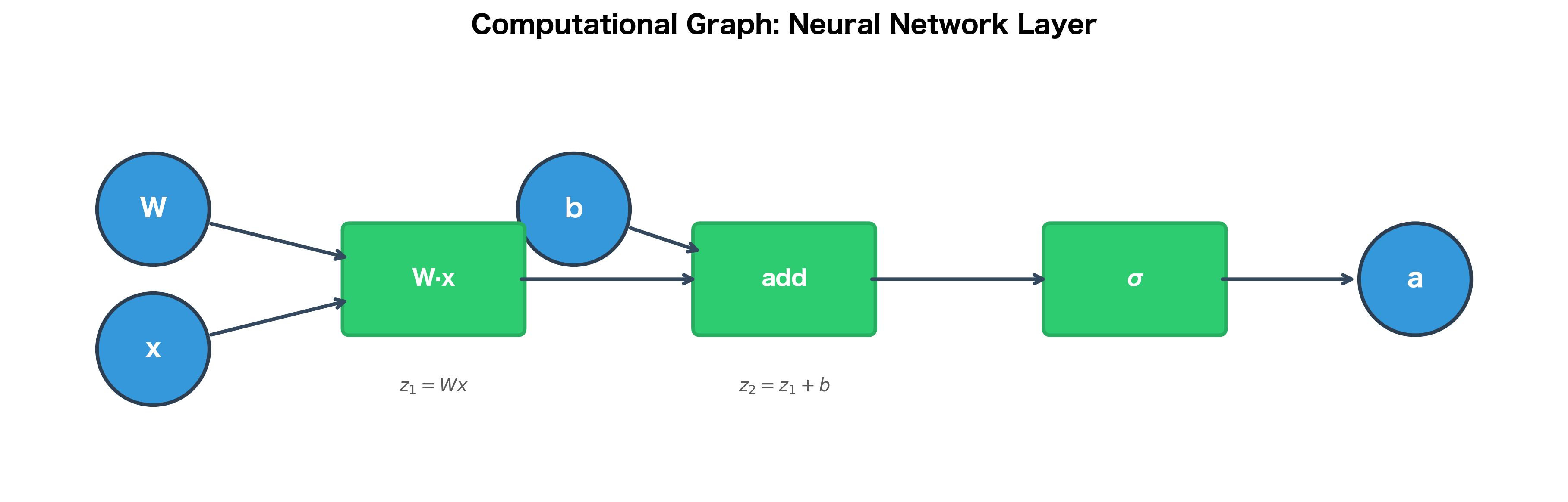
Each node in the graph represents an operation that we know how to differentiate. The power of computational graphs is that they make the structure of the computation explicit, which is exactly what we need for backpropagation.
Why Computational Graphs Matter
Computational graphs provide two crucial benefits for gradient computation:
-
Modularity: Each node has a well-defined local gradient. We don't need to derive the gradient of the entire network at once; we just need the gradient of each primitive operation.
-
Efficiency: By storing intermediate values during the forward pass, we can reuse them during the backward pass. This avoids redundant computation.
The forward pass computes values flowing left to right. The backward pass computes gradients flowing right to left. This symmetry is the essence of backpropagation.
The Chain Rule: Foundation of Backpropagation
We've seen how computational graphs break complex neural network computations into simple, modular operations. Now we face the central question: how do we compute the gradient of the loss with respect to every parameter in this graph?
The answer lies in the chain rule from calculus. To truly understand backpropagation, we need to see the chain rule not as a formula to memorize, but as a way of thinking about how influence propagates through a system of nested computations. Every operation in a neural network transforms its inputs in some way, and the chain rule tells us exactly how to trace the effect of any input change through all those transformations to the final output.
The Core Intuition: Tracing Influence Through Compositions
Before diving into formulas, let's build intuition with a physical analogy. Imagine a factory assembly line where raw materials pass through several processing stations, each transforming the product in some way, until a final item emerges. If you want to know how changing the raw material affects the final product, you need to trace that change through every station in sequence.
The same logic applies to neural networks. An input passes through layer after layer of transformations until it produces a loss value . To understand how affects , we trace the influence through each transformation, and the chain rule gives us the precise mathematical tool to do this.
Single Variable Chain Rule
Let's start with the simplest case: two functions arranged in a pipeline. First, transforms input into some intermediate value, then transforms that intermediate value into the final output. We write this composition as .
The question we want to answer is: if we nudge by a tiny amount, how much does the final output change?
Think of it as a two-stage amplification process:
-
Stage 1: The nudge to causes to change. If is very sensitive to (steep slope), a small change in produces a large change in . If is insensitive (flat slope), the change is small.
-
Stage 2: This change in then causes to change. Again, the magnitude depends on how sensitive is to its input.
The total effect is the product of these two sensitivities, as each stage amplifies (or attenuates) the signal from the previous stage:
where:
- : the total derivative, how much the final output changes per unit change in the original input . This is what we ultimately want to know.
- : the local gradient of the outer function, how sensitive is to changes in its immediate input . We can compute this knowing only the function , without caring about where came from.
- : the local gradient of the inner function, how sensitive is to changes in . We can compute this knowing only the function .
Why multiplication? If doubles any change in (i.e., ), and triples any change in (i.e., ), then a unit change in ultimately causes a unit change in . The effects compound multiplicatively.
This modularity is the key insight: we can break a complex derivative into a product of simple, local derivatives. Each function in the chain only needs to know how to differentiate itself with respect to its immediate inputs. It doesn't need to understand the entire pipeline.
Let's make this concrete with an example. Consider the composite function , which we can decompose as:
- Inner function:
- Outer function:
To find , we compute each local gradient and multiply:
- (derivative of )
- (derivative of )
The analytical gradient computed via the chain rule matches the numerical approximation to within , well within floating-point precision. This verification technique (comparing analytical gradients to numerical approximations) will become crucial when we implement backpropagation and need to verify our code is correct.
Multivariate Chain Rule: When Paths Diverge
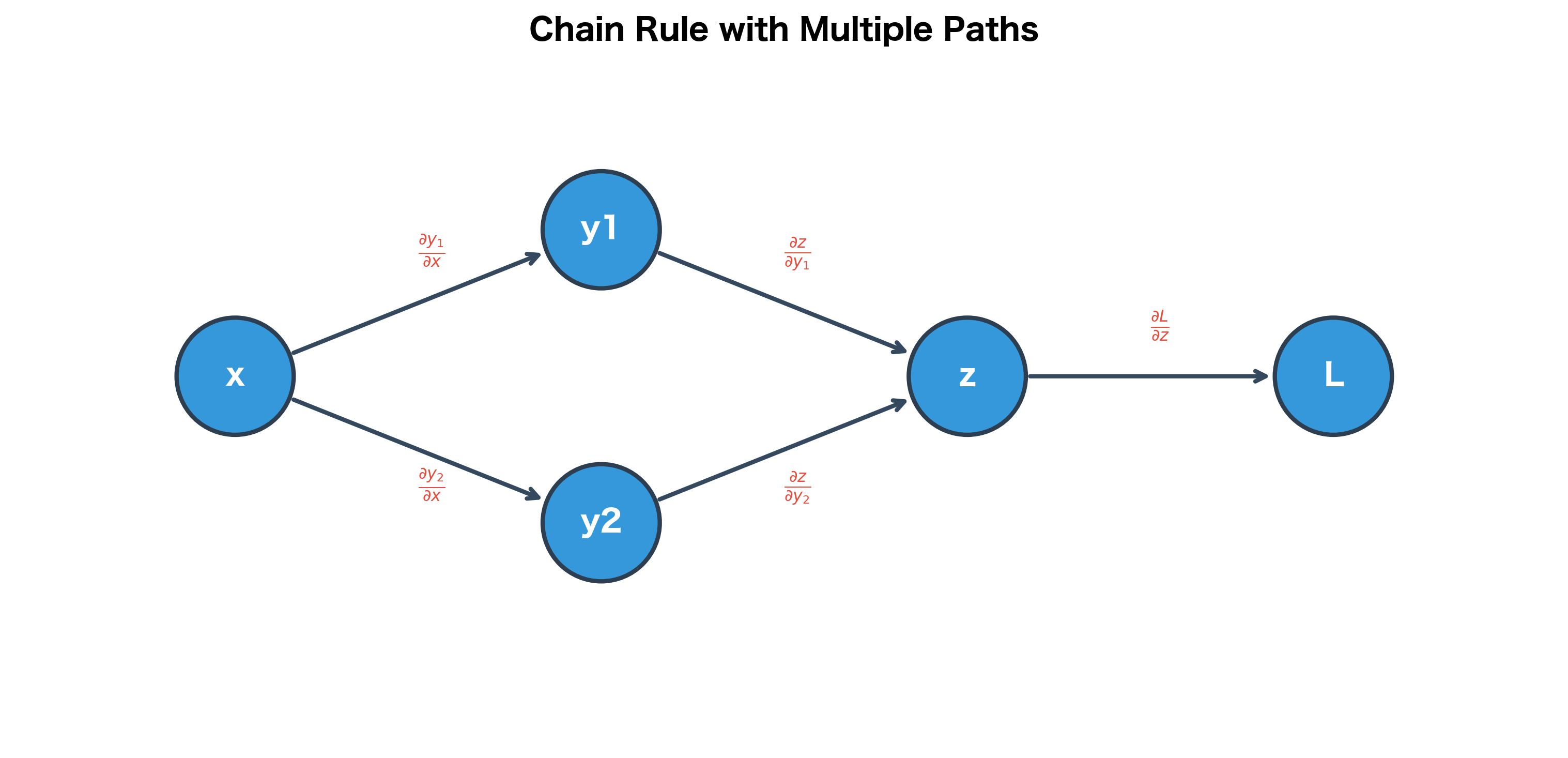
The single-variable chain rule handles a simple pipeline where one thing leads to another in a straight line. But neural networks are more complex: a single variable can influence the output through multiple intermediate pathways. This is where the multivariate chain rule becomes essential.
The Problem: Multiple Pathways of Influence
Consider a concrete scenario: in a neural network, a single weight might affect multiple neurons in the next layer, each of which contributes to the final loss. How do we account for all these influences?
Think of it like a river that splits into multiple tributaries before reaching the ocean. If you add a drop of dye at the source, it flows through all the tributaries. To measure the total amount of dye reaching the ocean, you must sum the contributions from each path.
The same principle applies to gradients: when a variable affects the output through multiple paths, we sum the contributions from each path. If changing increases the loss through one path and decreases it through another, the net effect is the sum of these opposing influences.
The Formula
Mathematically, if a variable affects the loss through several intermediate variables , the total gradient is:
Let's unpack each component:
- : the final loss, a single scalar value that we're trying to minimize
- : the variable we want to understand the influence of (e.g., a weight or bias)
- : all the intermediate values that directly depend on
- : how sensitive the loss is to changes in (this is computed by backpropagating from the output)
- : how sensitive is to changes in (this is computed locally)
Each term represents one "pathway of influence," the effect of on through the specific route via . The sum aggregates all these pathways.
Why This Matters for Neural Networks
This summation principle has profound implications for neural network training:
-
Gradient accumulation: When the same weight is used multiple times (as in recurrent networks processing sequences, or in architectures with shared weights), its gradient naturally accumulates contributions from each use.
-
Fan-out patterns: When a layer's output feeds into multiple downstream computations, the gradient flowing back must aggregate all these influences.
-
Batch processing: When we process multiple examples simultaneously, each example contributes to the gradient, and we sum (or average) these contributions.
Chain Rule on Computational Graphs: The Backpropagation Algorithm
Now we can see how the chain rule maps onto computational graphs, and this mapping is what transforms the abstract mathematics into a practical algorithm.
From Math to Algorithm
Recall that a computational graph represents a neural network's computation as a directed graph: nodes are operations, and edges show how data flows from inputs to outputs. During the forward pass, we compute values flowing from left to right. During the backward pass, we compute gradients flowing from right to left, from the loss back toward the inputs.
The key insight is that each node only needs to know its local gradient. A node doesn't need to understand the entire network; it just needs to know two things:
- Forward: How to compute its output from its inputs
- Backward: How to compute the gradient of its output with respect to its inputs
This locality is what makes backpropagation modular and scalable.
The Backward Pass Formula
For any node in the graph, the gradient of the loss with respect to follows directly from the multivariate chain rule:
where:
- : the loss function (a scalar value we're trying to minimize)
- : the current node whose gradient we're computing
- : the set of all nodes that directly receive as input (i.e., nodes downstream from )
- : the gradient of the loss with respect to each child node (already computed during backpropagation)
- : the local gradient, how much node 's output changes when changes
The Algorithm in Plain Language
This formula encodes a simple, elegant algorithm. For each node , working backward from the loss:
-
Look downstream: Find all nodes that use as an input (these are 's "children" in graph terminology)
-
Collect incoming gradients: Each child sends back a gradient signal , which tells us how sensitive the loss is to 's output
-
Scale by local sensitivity: Multiply each incoming gradient by , the local gradient that describes how much 's output changes when changes
-
Sum the contributions: Add up all these scaled gradients to get the total gradient at
Why This Works: The Recursive Structure
The beauty of this approach is its recursive structure. We start at the loss node, where (the loss is perfectly sensitive to itself). Then we work backward through the graph, layer by layer:
- Local information is sufficient: Each node computes its local gradient using only the operation type and values stored during the forward pass
- Gradients flow backward: Each node receives gradient signals from its children (which have already been computed) and passes gradient signals to its parents
- No global coordination needed: The algorithm is inherently parallel, and nodes at the same depth can compute their gradients simultaneously
This is the essence of backpropagation: a systematic, efficient way to apply the chain rule to computational graphs.
When a variable affects the loss through multiple paths, we sum the gradients from each path. This is why the chain rule involves a sum in the multivariate case.
Forward Pass: Computing Values
With the chain rule understood, we're ready to trace through an actual neural network. The forward pass propagates input data through the network, computing and storing intermediate values at each node. These stored values are essential for the backward pass; without them, we couldn't compute the local gradients.
Think of the forward pass as leaving breadcrumbs: as we compute each intermediate value, we save it for later use when gradients flow backward.
Step-by-Step Forward Computation
Let's trace through a concrete 2-layer network with the following architecture:
- Input: (2 features)
- Hidden layer: 3 neurons with ReLU activation
- Output layer: 1 neuron with sigmoid activation (for binary classification)
This small network is simple enough to trace by hand, yet complex enough to illustrate all the key concepts.
Now let's perform the forward pass, storing all intermediate values:
Notice how the ReLU activation zeroed out the negative pre-activation value in position 2 (z1[2] = -0.1 became a1[2] = 0). This sparsity is characteristic of ReLU networks, and it will have important implications for the backward pass, as we'll see shortly.
Computing the Loss
With the forward pass complete, we've arrived at a prediction. But how good is it? We need a way to quantify the error, and this is the role of the loss function.
For binary classification, we use binary cross-entropy (BCE), which measures how well the predicted probability matches the true label:
where:
- : the true label, either 0 or 1
- : the predicted probability from the sigmoid output, a value between 0 and 1
- : the natural logarithm
- : the loss value (always non-negative)
Understanding the Formula
This formula has an elegant interpretation that becomes clear when we consider the two cases:
When (positive class): The second term vanishes (since ), leaving .
- If (correct prediction): , so loss is small
- If (wrong prediction): , so loss is large
When (negative class): The first term vanishes (since ), leaving .
- If (correct prediction): , so loss is small
- If (wrong prediction): , so loss is large
The logarithm creates an asymmetric penalty: confident wrong predictions are punished severely, while confident correct predictions are rewarded with near-zero loss.
The loss of approximately 0.59 is moderate, not terrible, but clearly room for improvement. Our prediction of ~0.56 is below the target of 1.0, meaning the network is underconfident about the positive class. The loss quantifies this gap: a perfect prediction of 1.0 would yield a loss near 0, while our current prediction produces a loss that will drive gradient updates to increase the output probability. Now we need to compute gradients to reduce this loss.
Backward Pass: Computing Gradients
Now comes the heart of backpropagation. We've completed the forward pass, storing all intermediate values. We've computed the loss. Now we need to answer the fundamental question: how should we adjust each weight to reduce the loss?
The backward pass answers this by computing for every weight in the network. Armed with these gradients, we can update weights in the direction that decreases the loss.
The backward pass is like unwinding a ball of yarn. We start at the end (the loss) and work our way back to the beginning (the inputs), carefully tracking how each intermediate value influenced the final result. At each step, we apply the chain rule to decompose the complex derivative into simpler, local derivatives.
Step 1: Gradient of the Loss with Respect to the Prediction
Every backward pass begins at the loss function. The loss is our starting point because it's what we're trying to minimize. It's the "error signal" that will propagate backward through the network.
Before we can backpropagate through the network layers, we need to know: how does the loss change when the prediction changes? This is the gradient , the sensitivity of the loss to our prediction.
Let's derive this step by step, starting from the BCE formula:
Step 1: Write out the loss function:
This formula has two terms, but only one is ever "active" for a given example. When (positive class), the second term vanishes because . When (negative class), the first term vanishes because .
Step 2: Differentiate each term with respect to :
For the first term, we use the fact that :
For the second term, we need the chain rule because we're differentiating :
Step 3: Combine the terms:
Interpreting the Gradient
This formula reveals something important about how the loss "pushes" the prediction:
| Scenario | Gradient | Effect |
|---|---|---|
| , small (wrong) | (large negative) | Strong push to increase |
| , close to 1 (correct) | (small negative) | Gentle push to increase |
| , large (wrong) | (large positive) | Strong push to decrease |
| , close to 0 (correct) | (small positive) | Gentle push to decrease |
The loss function naturally provides stronger correction signals for more confident wrong predictions. This is exactly what we want: big mistakes get big corrections.
Step 2: Backpropagating Through Sigmoid
Now we need to push the gradient one step further back, through the sigmoid activation function. This is our first example of backpropagating through a nonlinearity, and it reveals a beautiful mathematical property that makes the combined BCE + sigmoid gradient remarkably simple.
The sigmoid function squashes any input into the range (0, 1). But what's its derivative? How sensitive is the sigmoid output to changes in its input?
Deriving the sigmoid derivative:
Step 1: Rewrite sigmoid using exponent notation for easier differentiation:
Step 2: Apply the chain rule. Let , so :
where:
- : a substitution variable to simplify the differentiation
- : the derivative of with respect to
- : the derivative of with respect to (the constant 1 vanishes, and )
The two negative signs cancel, giving us a positive result.
Step 3: Here's where it gets elegant. We can rewrite this messy expression entirely in terms of itself:
- Note that
- And
- Therefore:
This gives us the remarkably simple result:
where:
- : the sigmoid output, a value between 0 and 1
- : the complement of the sigmoid output
- : the product, which is maximized when
The Geometry of the Sigmoid Derivative
This formula has a beautiful geometric interpretation:
- Maximum at the midpoint: The derivative peaks at , where . This is where the sigmoid is steepest.
- Vanishes at the extremes: As or , the derivative approaches zero. The sigmoid flattens out.
This behavior has profound implications for training: when activations saturate near 0 or 1, gradients become tiny, making learning slow or impossible. This is the vanishing gradient problem for sigmoid activations.
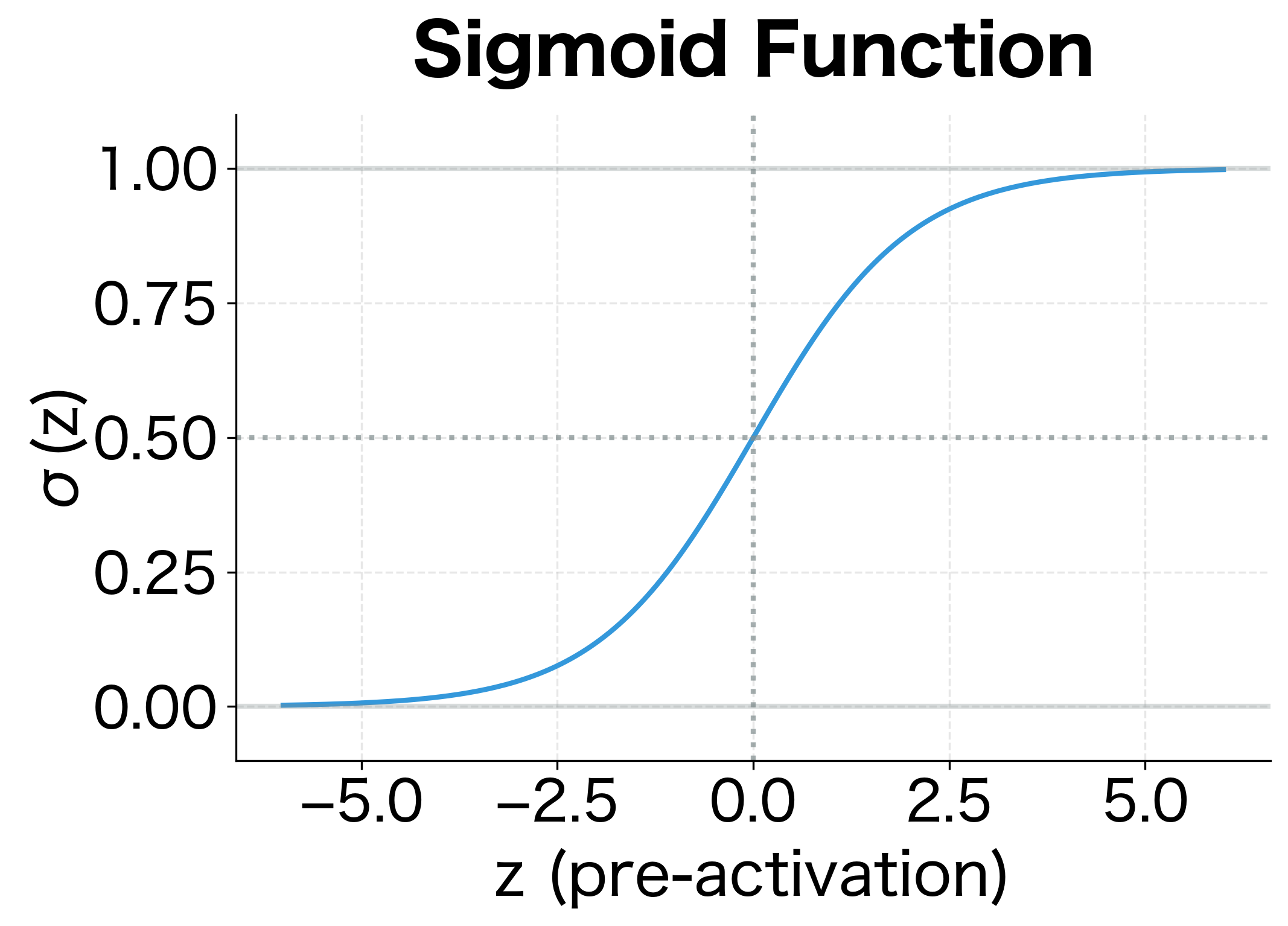
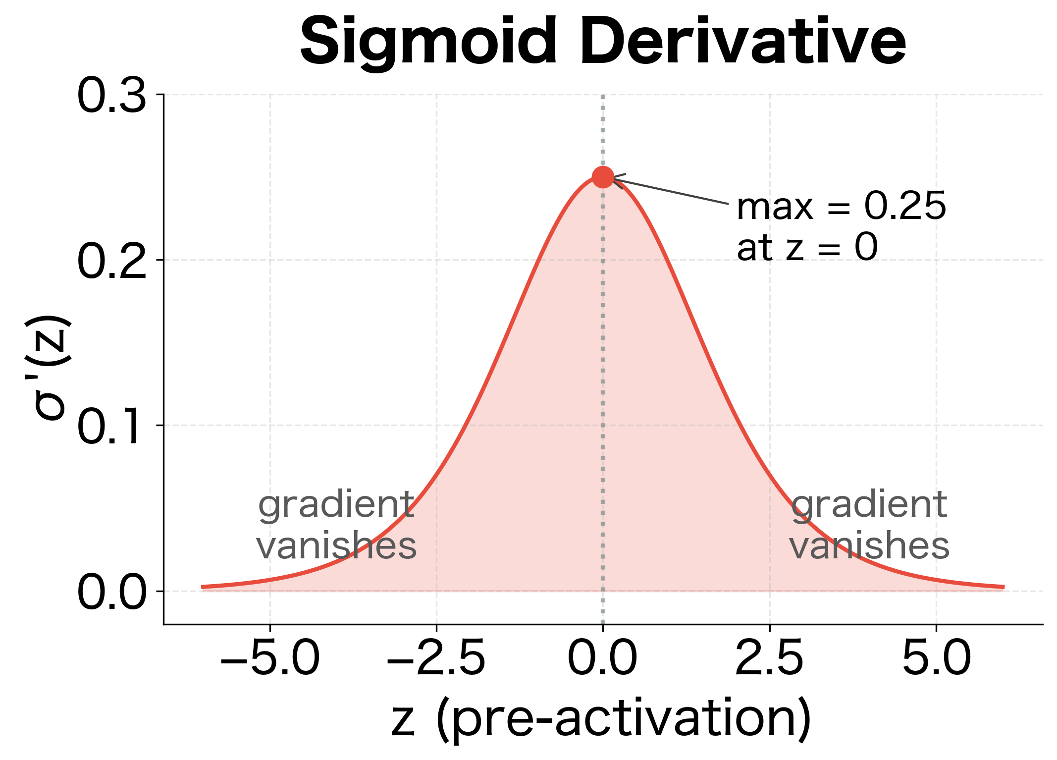
The visualization shows why sigmoid activations are problematic in deep networks. When the pre-activation is far from zero (either very positive or very negative), the derivative approaches zero, causing gradients to vanish during backpropagation. Only inputs near produce meaningful gradients.
Step 3: The Beautiful Cancellation (Combining BCE and Sigmoid)
Now comes the mathematical payoff that makes backpropagation through classification networks elegant. When we chain the BCE gradient with the sigmoid gradient using the chain rule, something remarkable happens:
where:
- : the pre-activation value (logit) before the sigmoid, i.e., the raw output of the linear layer
- : the sigmoid output (predicted probability)
- : the gradient of the loss with respect to the prediction (computed in the previous section)
- : the sigmoid derivative (computed above)
Substituting our expressions for and :
Let's expand this carefully:
The complex-looking derivatives collapse into something beautifully simple:
where:
- : the predicted probability (sigmoid output)
- : the true label (0 or 1)
- : the prediction error, which is positive when we over-predict and negative when we under-predict
This is remarkably simple: the gradient at the pre-sigmoid layer is just the prediction minus the target, the prediction error!
This elegant simplification is not a coincidence. Sigmoid and cross-entropy were designed to work together, and the mathematical complexity cancels out perfectly. The result is a gradient that's both easy to compute and deeply intuitive:
| Condition | Gradient | Interpretation |
|---|---|---|
| Positive | Push logit down to reduce prediction | |
| Negative | Push logit up to increase prediction | |
| Zero | Perfect prediction, no update needed |
The gradient magnitude is proportional to how wrong we are. A prediction of 0.9 when the target is 0 produces gradient 0.9, while a prediction of 0.6 produces gradient 0.6. Bigger mistakes get bigger corrections.
Step 4: Implementing the Full Backward Pass
Now we can implement the complete backward pass. The code below traces gradients from the loss back through both layers, computing gradients for all weights and biases.
Understanding the Backward Pass Step by Step
Let's trace through what just happened, connecting each computation to the chain rule:
1. Starting at the loss: We computed , the gradient at the output layer. This single number tells us how wrong our prediction was, and it's the "error signal" that will propagate backward.
2. Gradient for output weights (): We asked: "How does each weight in affect ?" Since , each weight is multiplied by the corresponding activation . By the chain rule:
3. Gradient for hidden activations (): To continue backpropagating, we need to know how affected the loss. Since , changing by a small amount changes by times that amount:
4. Through the ReLU (): The ReLU function has a simple derivative:
This acts as a gate: gradients pass through unchanged for positive pre-activations, but are completely blocked for negative ones. The gradient becomes , where denotes element-wise multiplication.
5. Gradient for hidden weights (): Following the same pattern as the output layer:
The ReLU Gate and "Dying Neurons"
Notice how the ReLU gradient acts as a gate. Where , the gradient passes through unchanged. Where , the gradient is blocked (zeroed). In our example, the third neuron had , so its gradient was blocked entirely.
This is the "dying ReLU" phenomenon: neurons that never activate don't receive gradient updates. If a neuron's pre-activation is always negative (perhaps due to poor initialization or a large negative bias), it will never learn. This is why variants like Leaky ReLU (which allow small gradients for negative inputs) are sometimes preferred.
Understanding the Gradient Shapes
Each gradient has a specific shape that matches its corresponding parameter:
| Parameter | Shape | Gradient Shape | Explanation |
|---|---|---|---|
| W1 | (3, 2) | (3, 2) | 3 hidden neurons, 2 inputs |
| b1 | (3, 1) | (3, 1) | One bias per hidden neuron |
| W2 | (1, 3) | (1, 3) | 1 output, 3 hidden inputs |
| b2 | (1, 1) | (1, 1) | One bias for output |
The gradient shapes always match the parameter shapes. This must be true because we subtract gradients from parameters during the update step, and subtraction requires matching shapes.
Verifying Gradients: The Gradient Checking Technique
We've derived and implemented the backward pass analytically. But how do we know we got it right? A single sign error or transposed matrix can silently produce wrong gradients, leading to a network that trains poorly or not at all.
The solution is gradient checking: verify analytical gradients against numerical approximations. The idea is simple: perturb each parameter slightly and measure how the loss changes. If our analytical gradient is correct, it should match this numerical estimate.
The Centered Difference Formula
The centered difference formula gives an accurate numerical approximation:
where:
- : a single scalar parameter we're checking
- : a small perturbation, typically
- : the loss computed with increased by
- : the loss computed with decreased by
Why centered difference? The one-sided formula has error. The centered difference cancels first-order error terms, giving accuracy, typically 5-7 orders of magnitude better for the same .
The analytical and numerical gradients match to within , well within the expected precision for . This confirms our backpropagation implementation is correct.
Gradient checking is computationally expensive (it requires two forward passes per parameter), so don't use it during normal training. Instead, use it:
- When implementing a new layer or activation function
- When debugging a network that won't train
- When porting code to a new framework
- Once, after implementing backpropagation, to verify correctness
A relative error below typically indicates correct implementation. Errors above suggest a bug.
Gradient Accumulation
When a variable is used multiple times in a computation, its gradient accumulates contributions from all uses. This is the multivariate chain rule in action.
Why Gradients Accumulate
Consider a weight matrix used to process a batch of examples. Each example contributes to the total loss, and each contribution produces its own gradient for . Since the total loss is the average (or sum) of individual losses, the total gradient is the sum of individual gradients:
where:
- : the batch size (number of examples processed together)
- : the loss contribution from example
- : the gradient of the loss with respect to from example alone, a matrix with the same shape as
- : the total gradient, summed across all examples
This summation happens automatically in matrix operations when processing batches. When we compute , the matrix multiplication implicitly sums over the batch dimension, and the factor converts the sum to an average.
Batch Processing and Gradient Accumulation
Let's see how gradient accumulation works with a batch of examples:
The predictions show mixed accuracy on this random batch, with some examples classified correctly while others are not. This is expected since we're using the same small network trained on XOR, which doesn't generalize to random inputs. The key observation is the gradient shape: dW2 has shape (1, 3), matching W2 exactly. The matrix multiplication dz2 @ a1.T (shapes 1×4 and 4×3) automatically sums over the batch dimension, and the factor converts this sum to an average, making the effective learning rate independent of batch size.
Visualizing Gradient Flow
Let's visualize how gradients flow backward through our network:
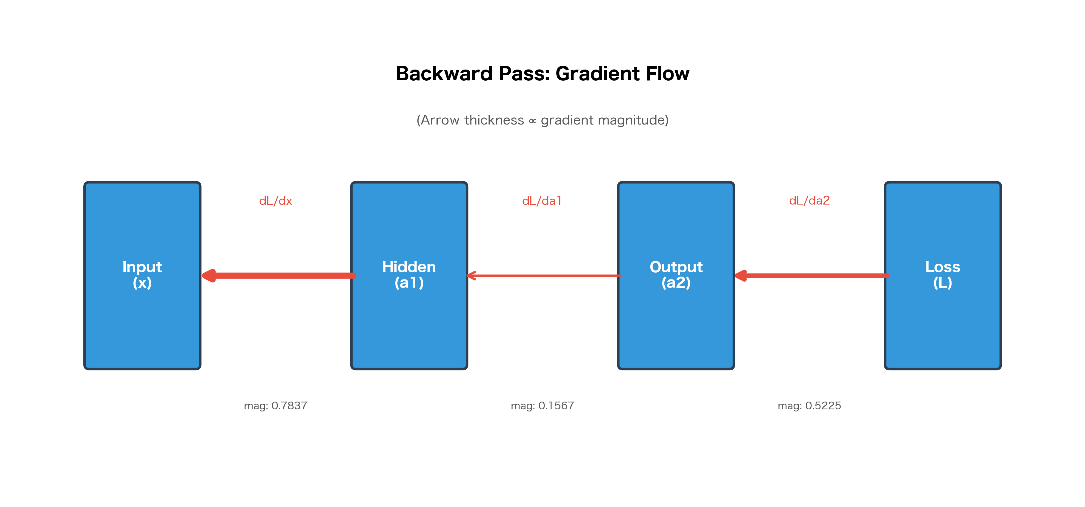
The gradient magnitudes can vary significantly across layers. In deep networks, this can lead to vanishing gradients (gradients become tiny in early layers) or exploding gradients (gradients become huge). Techniques like batch normalization, residual connections, and careful initialization help mitigate these issues.
Tracking Gradients During Training
Let's train a deeper network and monitor how gradient magnitudes evolve across layers and epochs:
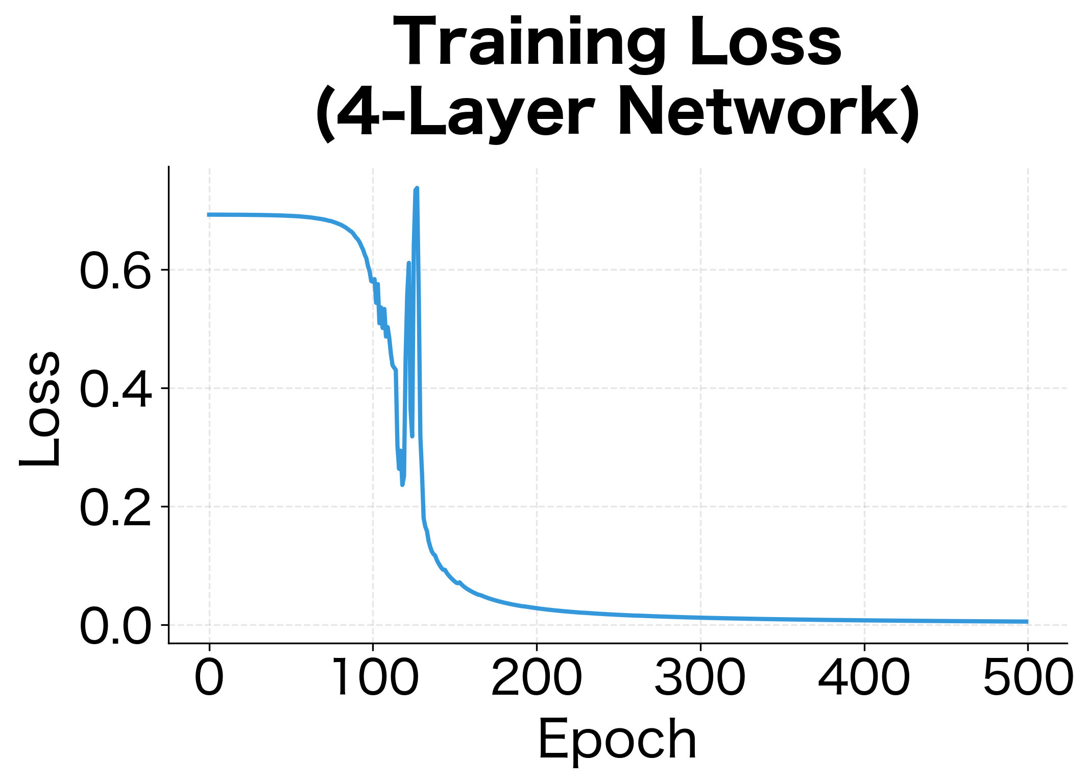
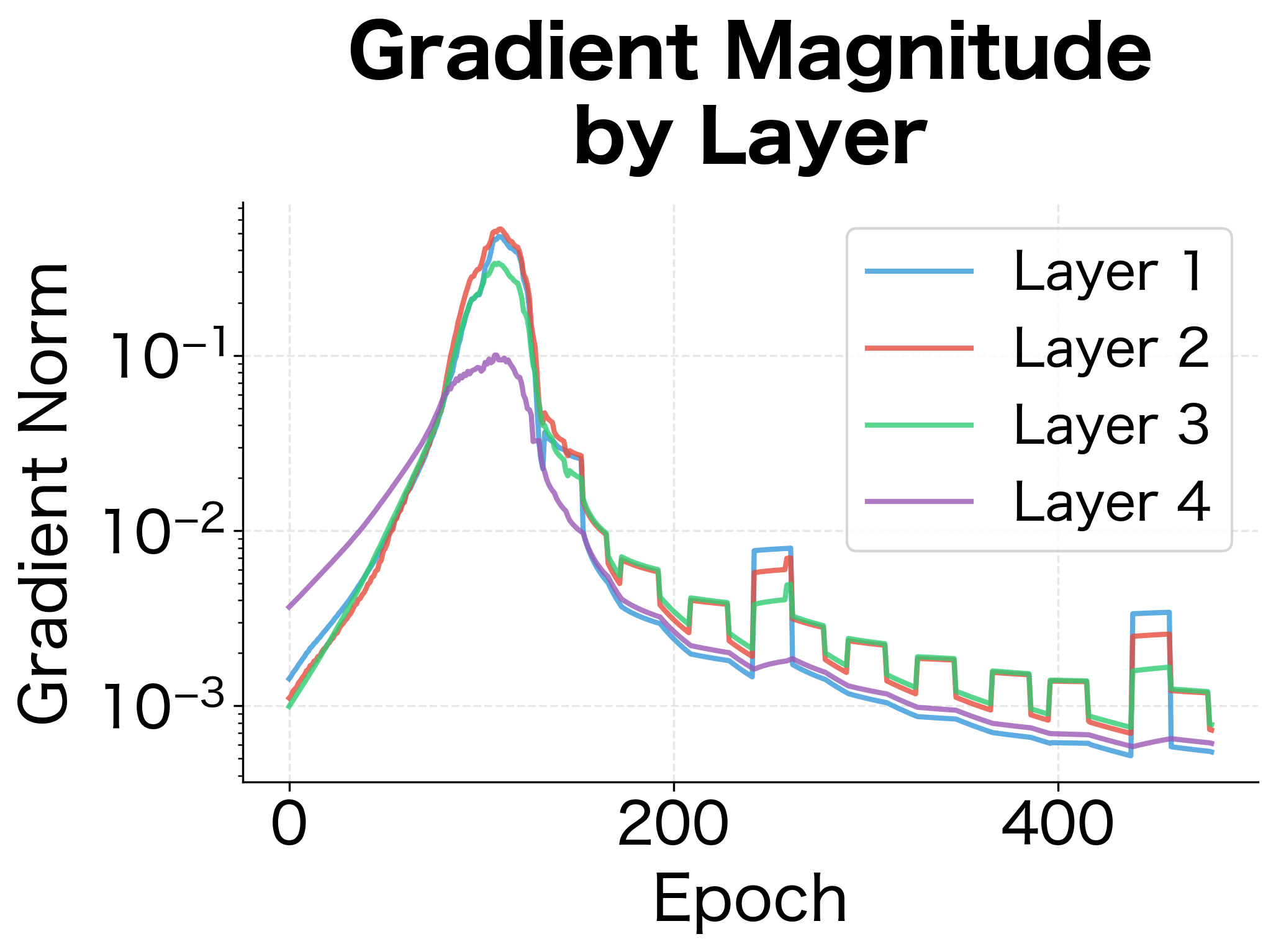
The gradient magnitude plot reveals a key pattern: gradients tend to be smaller in earlier layers (closer to the input). This is the vanishing gradient effect in action. Each layer's backward pass multiplies gradients by weight matrices and activation derivatives, which can compound to shrink gradients exponentially. In this 4-layer network, the effect is modest, but in networks with 50+ layers, it becomes severe without architectural interventions like residual connections.
Complexity Analysis
Understanding the computational cost of backpropagation helps explain why it's so efficient and why training is more expensive than inference.
Time Complexity
For a single layer with inputs and outputs:
| Operation | Forward | Backward |
|---|---|---|
| Matrix multiply | ||
| Bias addition | ||
| Activation | ||
| Total per layer |
The backward pass has the same asymptotic complexity as the forward pass. This is a remarkable property: computing all gradients costs roughly the same as computing the output.
For a network with layers and average layer size , the total time complexity is:
where:
- : number of layers
- : average number of neurons per layer
- : comes from the matrix multiplication at each layer (an weight matrix multiplied by an -dimensional vector)
This holds for both forward and backward passes. The constant factor for backward is typically 2-3× the forward pass due to additional operations (computing gradients for both weights and activations).
Space Complexity
Backpropagation requires storing intermediate activations from the forward pass because these values are needed to compute gradients during the backward pass. For a batch of size through layers with average layer size neurons:
where:
- : batch size (number of examples processed together)
- : number of layers in the network
- : average number of neurons per layer
The total number of stored values is approximately , since we store one activation value per neuron per example. This memory requirement is why:
- Larger batch sizes require more GPU memory
- Deeper networks require more memory
- Techniques like gradient checkpointing trade compute for memory by recomputing activations during the backward pass
For this small network with a batch size of 32, storing activations requires only about 158 KB. However, this scales linearly with both batch size and network depth. A ResNet-50 with 50 layers and batch size 256 would require gigabytes of activation memory. The input layer (784 neurons for MNIST images) dominates the memory footprint here, but in deeper networks, the cumulative storage across many hidden layers becomes the bottleneck.
Why Backpropagation is Efficient
Before backpropagation, computing gradients required either:
-
Numerical differentiation: Perturb each of parameters and measure loss change. Cost: . For networks with millions of parameters, this is prohibitively expensive.
-
Symbolic differentiation: Derive analytical gradient formulas. This produces expressions that grow exponentially with network depth due to repeated subexpressions.
Backpropagation achieves complexity by:
- Computing gradients in a single backward sweep
- Reusing intermediate values computed during the forward pass
- Avoiding redundant computation through dynamic programming
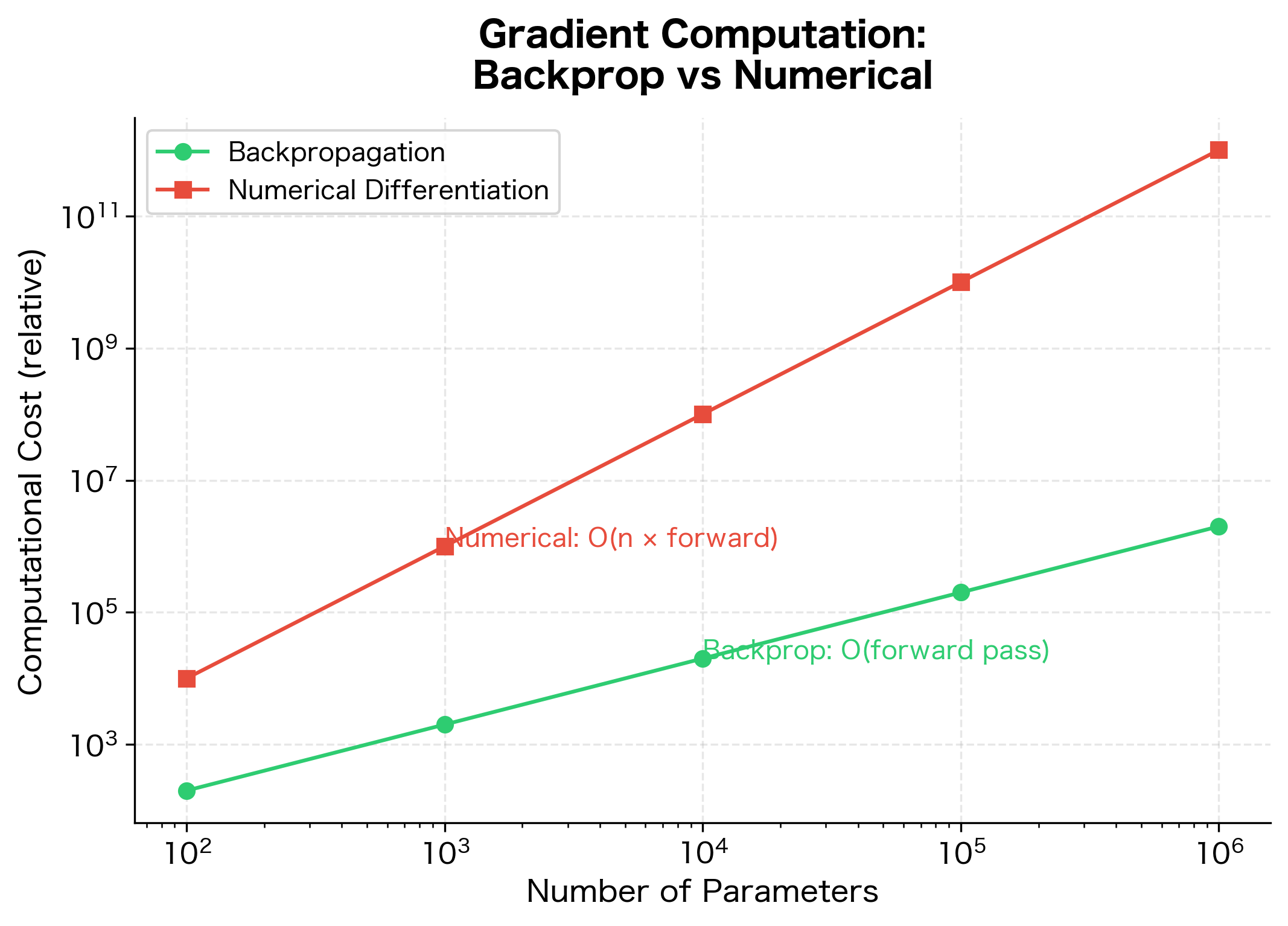
The gap between the two methods grows linearly with network size. For a network with 1 million parameters, numerical differentiation would be roughly 1 million times slower than backpropagation.
Automatic Differentiation
Modern deep learning frameworks like PyTorch and TensorFlow implement automatic differentiation (autodiff), which automates the backpropagation process. Understanding autodiff helps you use these frameworks more effectively.
How Autodiff Works
Autodiff systems build a computational graph during the forward pass, recording every operation. During the backward pass, they traverse this graph in reverse, applying the chain rule at each node.
There are two modes of autodiff:
-
Forward mode: Computes for all outputs with respect to one input . Efficient when there are few inputs and many outputs.
-
Reverse mode: Computes for all inputs with respect to one output . Efficient when there are many inputs and few outputs (like a scalar loss).
Neural network training uses reverse mode because we have many parameters (inputs) and one loss (output).
PyTorch's Autograd
PyTorch implements reverse-mode autodiff through its autograd system. Every tensor operation is recorded, and calling .backward() on a scalar triggers gradient computation.
PyTorch's gradients match our manual implementation exactly. The framework handles all the bookkeeping automatically, tracking operations and computing gradients with a single .backward() call.
The Computational Graph in PyTorch
PyTorch builds a dynamic computational graph, meaning the graph is constructed fresh for each forward pass. This allows for dynamic control flow (if statements, loops) that can change based on input data.
Despite the conditional logic that selects different activation functions at runtime, PyTorch successfully computed gradients by building the computational graph on-the-fly during the forward pass. This dynamic graph capability is what enables models with variable-length inputs (like RNNs processing sentences of different lengths), recursive structures (like tree-structured neural networks), and attention mechanisms where computation paths depend on the data.
Implementing Backpropagation from Scratch
We've traced through backpropagation step by step, derived the key formulas, and verified them numerically. Now let's consolidate everything into a complete, working implementation.
The NeuralNetwork class below encapsulates the full training loop: forward pass, loss computation, backward pass, and parameter updates. This is the same algorithm that powers deep learning frameworks, but we're implementing it explicitly to understand every detail.
Training on a Simple Dataset: The XOR Problem
To verify our implementation works, let's train on the XOR problem, a classic test case that single-layer networks cannot solve. XOR requires learning a nonlinear decision boundary, making it the perfect sanity check for our multi-layer network.
The network successfully learns XOR! All four examples are classified correctly, with predictions very close to the targets. This demonstrates that our backpropagation implementation is working correctly. The gradients are flowing properly and the weights are being updated in the right direction.
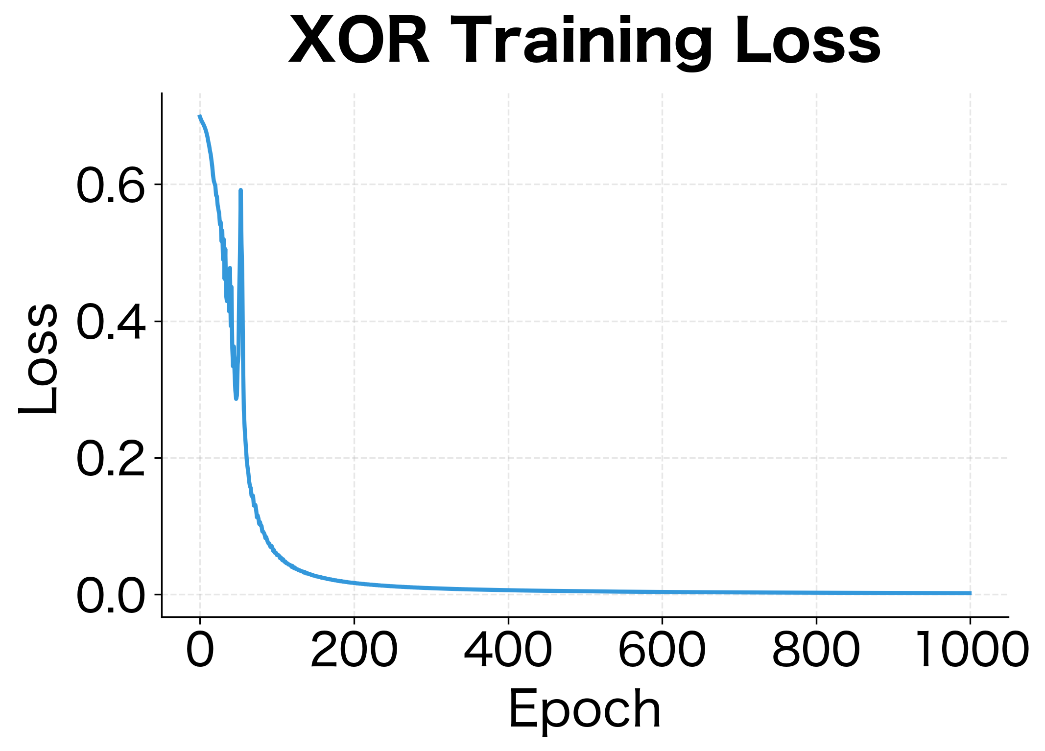
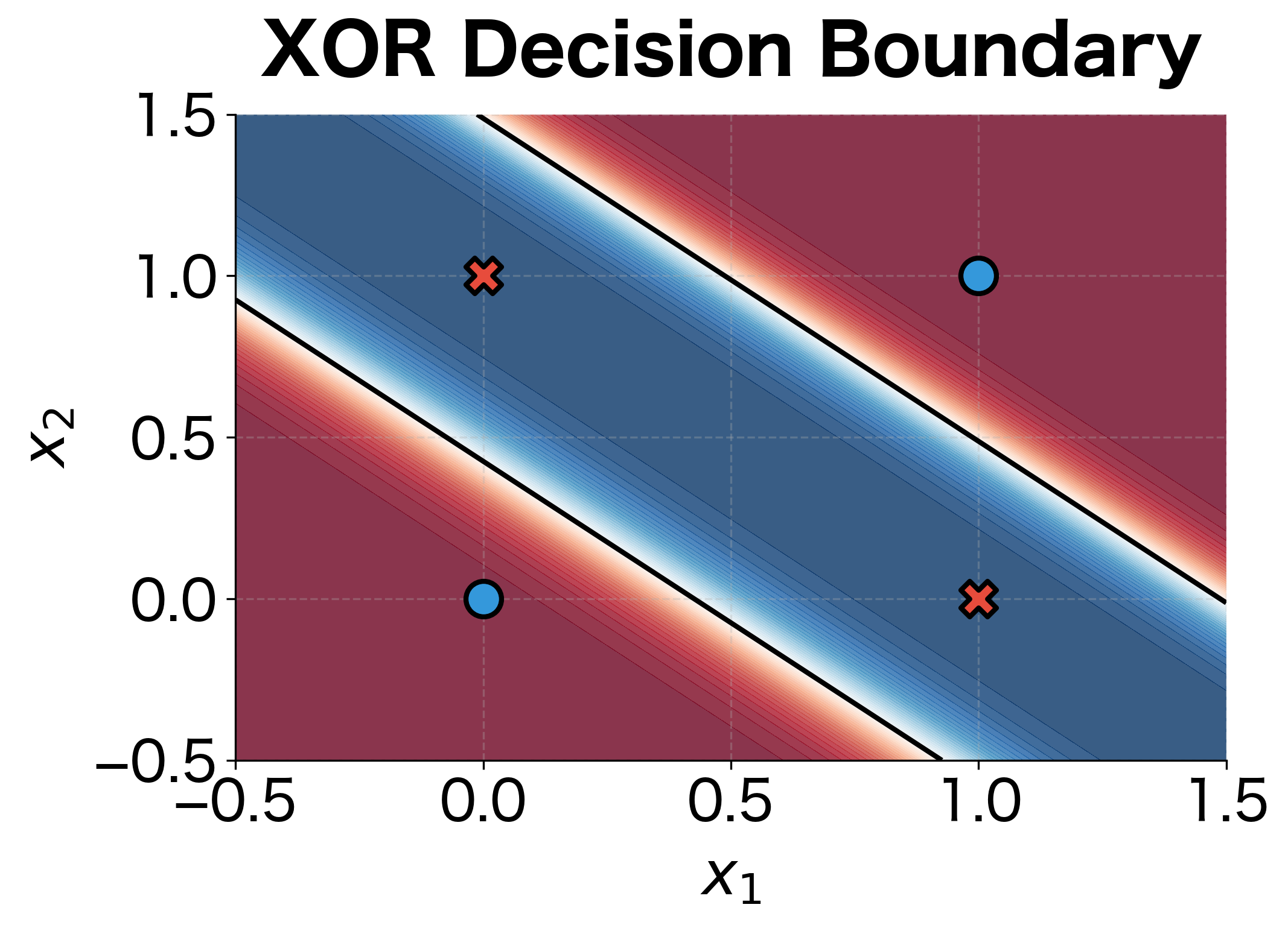
The loss curve shows rapid initial learning followed by gradual refinement, a typical pattern in neural network training. The decision boundary visualization reveals how the network solves XOR: it creates a curved region that separates the (0,1) and (1,0) points (class 1, red) from (0,0) and (1,1) (class 0, blue).
This curved boundary is impossible for a linear classifier to achieve. The hidden layer transforms the input space, making the originally non-linearly-separable problem linearly separable in the hidden representation. This is the power of multi-layer networks with nonlinear activations.
Common Pitfalls and Debugging
Implementing backpropagation correctly requires attention to detail. Here are common issues and how to diagnose them.
Gradient Checking
Always verify your gradients numerically when implementing new layers:
Common Bugs and Symptoms
| Symptom | Possible Cause | Solution |
|---|---|---|
| Loss doesn't decrease | Learning rate too small or gradients wrong | Check gradient numerically; try larger LR |
| Loss explodes to NaN | Learning rate too large or numerical overflow | Reduce LR; add gradient clipping |
| Gradients are all zero | Dead ReLUs or vanishing gradients | Use Leaky ReLU; check initialization |
| Gradients don't match numerical | Shape mismatch or wrong formula | Print shapes; verify math step by step |
Shape Debugging
Shape errors are the most common bugs. Always verify:
The shapes reveal the network's structure: 4 examples (batch size) flow through 2 input features to 4 hidden neurons to 1 output. Notice that dW1 has shape (4, 2), exactly matching W1. This is required because gradient descent subtracts gradients from parameters element-wise. Similarly, dW2 matches W2 at (1, 4). If any gradient shape differs from its parameter shape, there's a bug in the backward pass.
Limitations and Practical Considerations
Backpropagation is powerful but has important limitations that affect how we design and train neural networks.
Vanishing and Exploding Gradients
In deep networks, gradients can become exponentially small (vanishing) or large (exploding) as they propagate backward. To understand why, consider a simplified network with layers where each layer multiplies the gradient by some factor during backpropagation. After passing through all layers, the gradient at the first layer is scaled by:
where:
- : the average gradient scaling factor per layer, determined by the product of weight magnitudes and activation derivatives. For sigmoid activations, this is typically less than 1 since .
- : the number of layers the gradient must traverse
- : the cumulative scaling effect, which grows or shrinks exponentially with depth
If (e.g., ), then shrinks exponentially: for layers, , meaning gradients nearly vanish. If (e.g., ), then grows exponentially: , meaning gradients explode.
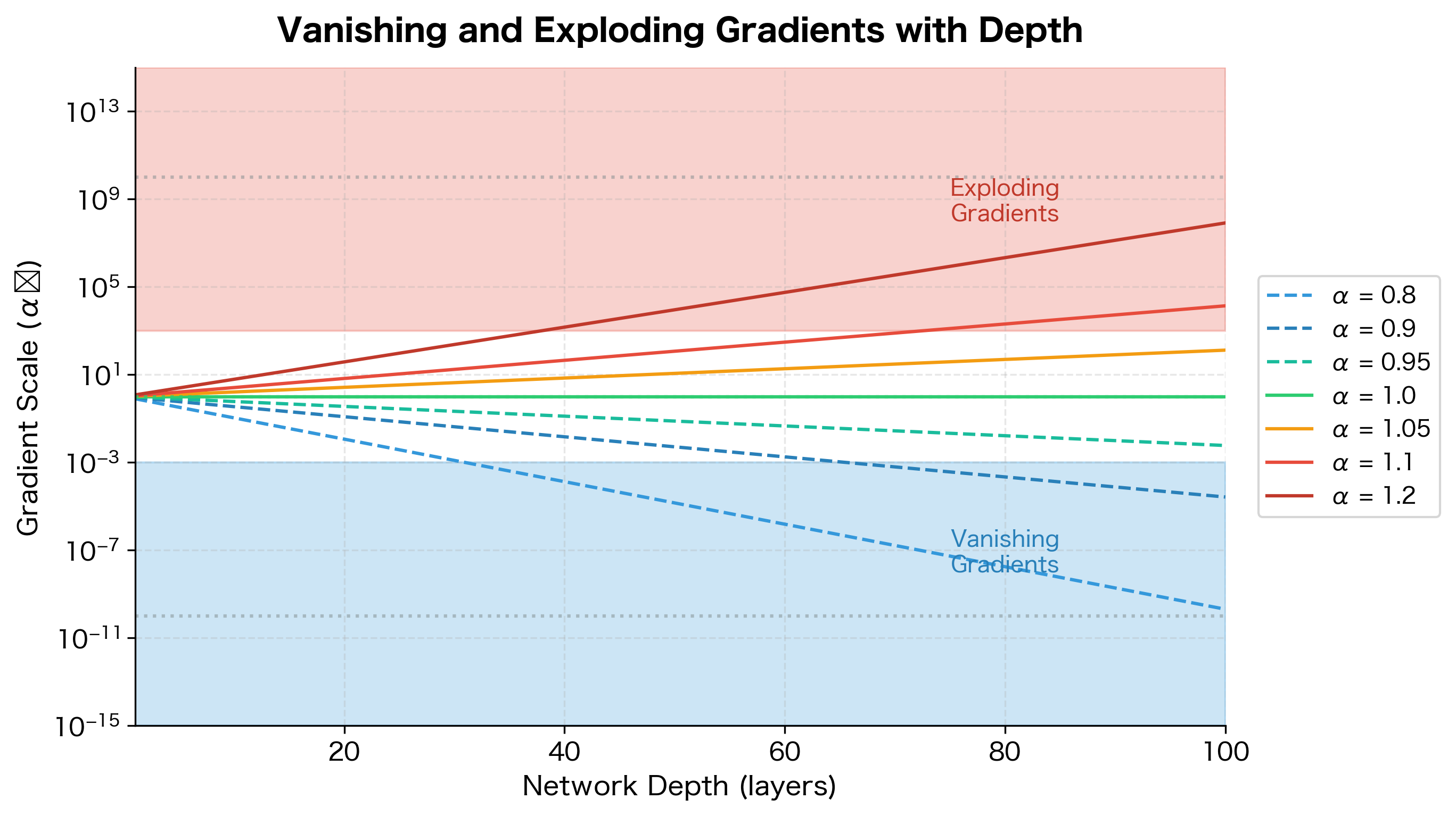
The visualization makes the problem visceral: even a 5% deviation from leads to gradients that are 100× too small or too large after just 100 layers. This is why deep networks were considered untrainable before techniques like residual connections, which allow gradients to bypass layers and maintain .
This problem is particularly severe with sigmoid and tanh activations, whose derivatives are bounded below 1. ReLU helps because its derivative is exactly 1 for positive inputs, but "dead" ReLU neurons (always outputting 0) still block gradient flow entirely.
Modern solutions include:
- Residual connections: Allow gradients to flow directly through skip connections
- Batch normalization: Stabilizes activations and gradients
- Careful initialization: Xavier or He initialization keeps gradients in a healthy range
- Gradient clipping: Caps gradient magnitude to prevent explosions
Memory Requirements
Backpropagation requires storing all intermediate activations from the forward pass. For large models and batch sizes, this memory cost can be prohibitive. A model with 1 billion parameters might need 10-20 GB just for activations during training, on top of the memory for parameters and gradients.
Gradient checkpointing trades compute for memory by recomputing activations during the backward pass instead of storing them all. Instead of storing all layers of activations, we only store activations at every layers (the "checkpoints"). During the backward pass, we recompute the activations between checkpoints as needed. This reduces memory from to stored activation layers, at the cost of roughly doubling compute time (since we recompute most forward activations once during the backward pass).
Local Minima and Saddle Points
Backpropagation finds directions that decrease the loss locally, but it doesn't guarantee finding the global minimum. In high-dimensional spaces, saddle points (where gradients are zero but it's not a minimum) are far more common than local minima. The good news is that most saddle points in neural networks are "escapable" with enough noise from stochastic gradient descent.
To visualize what gradient descent "sees," let's plot a 2D slice of the loss landscape for our XOR network by varying two weights while keeping others fixed:
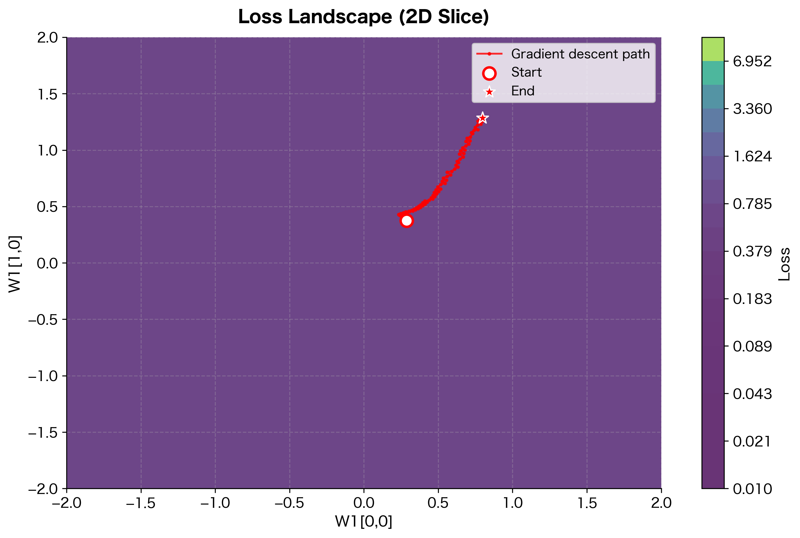
The loss landscape reveals the non-convex nature of neural network optimization. Gradient descent follows the steepest downhill direction at each step, navigating through valleys toward a minimum. The path isn't straight because the gradient direction changes as we move through the landscape. In higher dimensions (where real networks live), the landscape is even more complex, with many saddle points and local minima. Empirically, most local minima in deep networks achieve similar loss values.
Despite these limitations, backpropagation remains the foundation of deep learning. Its efficiency makes training billion-parameter models practical, and its modularity allows researchers to easily experiment with new architectures and loss functions.
Summary
Backpropagation is the algorithm that makes deep learning possible. By systematically applying the chain rule from output to input, it computes gradients for all parameters in time proportional to a single forward pass. We've traced through every step of this algorithm, from mathematical foundations to working implementation.
The Core Ideas:
-
Computational graphs decompose complex neural network computations into simple, modular operations. Each node knows only how to compute its output and its local gradient, with no global knowledge required.
-
The chain rule tells us how to trace influence through compositions. For a single path, we multiply derivatives. For multiple paths, we sum the contributions:
where:
- : the loss function
- : the variable whose gradient we want (e.g., a weight)
- : intermediate variables that depend on
- The sum aggregates contributions from all paths connecting to
-
The forward pass computes values from input to output, storing intermediate results. The backward pass computes gradients from output to input, using those stored values.
-
The BCE + sigmoid simplification shows how careful mathematical design pays off: the complex gradient collapses to the simple form .
Practical Takeaways:
- Gradient checking (comparing analytical gradients to numerical approximations) is essential for verifying implementations
- Gradient accumulation naturally handles batch processing and shared weights
- Time complexity of backward pass matches forward pass:
- Automatic differentiation frameworks like PyTorch implement all of this automatically, building computational graphs on-the-fly
The backward pass produces gradients, but we still need to decide how to use them. The next chapter explores stochastic gradient descent and its variants, which use these gradients to actually update parameters and train the network.
Key Parameters
When implementing or using backpropagation, several parameters affect correctness and numerical stability:
Numerical Stability:
- Epsilon for gradient checking: Use to . Too small causes floating-point errors; too large gives inaccurate approximations.
- Clipping for sigmoid/softmax: Clip inputs to prevent overflow () and outputs to prevent .
Memory Management:
- Batch size: Larger batches require more memory for storing activations. Memory scales as .
- Gradient checkpointing: Trade 2× compute for memory reduction in -layer networks.
Gradient Health:
- Gradient magnitude: Monitor gradient norms during training. Healthy gradients typically have norms between and .
- Gradient clipping threshold: Common values are 1.0 to 5.0 for the maximum gradient norm.
Initialization:
- Xavier/Glorot initialization: Scale weights by for tanh/sigmoid activations, where is the number of input neurons (fan-in) and is the number of output neurons (fan-out). This keeps the variance of activations roughly constant across layers.
- He initialization: Scale weights by for ReLU activations, where is the number of input neurons to the layer. The factor of 2 accounts for ReLU zeroing out half the inputs on average.
Quiz
Ready to test your understanding? Take this quick quiz to reinforce what you've learned about backpropagation and gradient computation in neural networks.

Comments