AdamW Optimizer: Decoupled Weight Decay for Deep Learning

Adam transformed deep learning optimization by combining momentum with adaptive learning rates. Yet researchers noticed something peculiar: the regularization techniques that worked beautifully with SGD seemed less effective with Adam. Models trained with Adam often generalized worse than those trained with vanilla SGD plus weight decay.

The culprit? A subtle but critical difference between L2 regularization and weight decay. For most optimizers, these two techniques are mathematically equivalent. But Adam's adaptive learning rates break this equivalence, causing L2 regularization to behave in unexpected ways. AdamW, introduced by Loshchilov and Hutter in 2017, fixes this problem by decoupling weight decay from the gradient-based update. The result is an optimizer that combines Adam's fast convergence with proper regularization, now the default choice for training transformers and large language models.

Before diving into AdamW, we need to understand the subtle distinction between L2 regularization and weight decay. These terms are often used interchangeably, but they represent different approaches to the same goal: preventing overfitting by penalizing large weights.

L2 regularization adds a penalty term to the loss function based on the squared magnitude of the weights:

where:

• $\mathcal{L}$: the original loss function (such as cross-entropy or mean squared error)
• $\mathcal{L}_{\text{reg}}$: the regularized loss that we actually minimize
• $w$: the weight vector containing all trainable parameters in the network
• $\|w\|^2 = \sum_i w_i^2$: the squared L2 norm of the weights
• $\lambda$: the regularization strength hyperparameter (larger values penalize large weights more heavily)
• $\frac{1}{2}$: a convenience factor that simplifies the gradient calculation

When we compute the gradient of this regularized loss with respect to the weights, the chain rule gives us:

where:

• $\nabla_w \mathcal{L}$: the gradient of the original loss with respect to weights
• $\lambda w$: the regularization gradient, which points in the direction of the current weights

The regularization contributes an additional term $\lambda w$ to the gradient. This means larger weights produce larger gradients, pushing the optimizer to shrink them during training.

Weight decay takes a different approach. Instead of modifying the loss function, it directly modifies the weight update:

where:

• $w_t$: the weight vector at time step $t$
• $w_{t+1}$: the updated weight vector after one optimization step
• $\eta$: the learning rate
• $\nabla_w \mathcal{L}$: the gradient of the loss with respect to weights
• $\lambda$: the weight decay coefficient
• $\eta \lambda w_t$: the decay term that shrinks weights toward zero

We can factor this equation to see the decay more explicitly:

The factor $(1 - \eta \lambda)$ is slightly less than one, so at each step we multiply the weights by this factor before applying the gradient update. This causes weights to "decay" toward zero over time. The hyperparameter $\lambda$ controls how quickly this decay happens.

For standard SGD, these two formulations produce identical updates. With L2 regularization, the SGD update becomes:

The left side shows the update using the regularized gradient $(\nabla_w \mathcal{L} + \lambda w_t)$, while the right side expands to match the weight decay formulation exactly. Because SGD applies the same learning rate $\eta$ uniformly to all gradient components, the regularization strength $\lambda$ has the same effect in both cases. This mathematical equivalence is why practitioners historically treated the terms as synonyms.

Adam's adaptive learning rates fundamentally change the relationship between L2 regularization and weight decay. To see why, recall Adam's update rule:

where:

• $w_t$: the weight vector at time step $t$
• $\eta$: the base learning rate
• $\hat{m}_t$: the bias-corrected first moment estimate (exponential moving average of gradients)
• $\hat{v}_t$: the bias-corrected second moment estimate (exponential moving average of squared gradients)
• $\epsilon$: a small constant for numerical stability (typically $10^{-8}$)
• $\frac{\eta}{\sqrt{\hat{v}_t} + \epsilon}$: the effective learning rate, which adapts per-parameter based on gradient history

The key insight is that each parameter gets divided by $\sqrt{\hat{v}_t}$, which depends on the history of gradients for that parameter. Parameters with consistently large gradients have large $\hat{v}_t$ values, which reduces their effective learning rate.

When we use L2 regularization with Adam, the gradient becomes $\nabla_w \mathcal{L} + \lambda w$. This regularization term enters Adam through both moment estimates:

where:

• $m_t$: the first moment estimate (momentum), now incorporating the regularization term
• $v_t$: the second moment estimate, now incorporating the squared regularization term
• $\beta_1$: the exponential decay rate for the first moment (typically 0.9)
• $\beta_2$: the exponential decay rate for the second moment (typically 0.999)
• $\lambda w$: the L2 regularization gradient added to the loss gradient

The problem lies in the second moment $v_t$. For parameters with large weights, the term $(\nabla_w \mathcal{L} + \lambda w)^2$ increases $v_t$, which in turn decreases the effective learning rate $\frac{\eta}{\sqrt{\hat{v}_t} + \epsilon}$ for those parameters.

This creates a problematic feedback loop: L2 regularization is supposed to push large weights toward zero, but Adam's adaptation reduces the update magnitude for parameters that receive large gradients. The regularization signal gets dampened precisely where it should be strongest.

True weight decay sidesteps Adam's adaptive mechanism entirely. Instead of modifying the gradient, we apply decay directly to the weights after the Adam update:

This equation has two distinct terms after $w_t$:

• $\frac{\eta}{\sqrt{\hat{v}_t} + \epsilon} \hat{m}_t$: the standard Adam update, which adapts to gradient history
• $\eta \lambda w_t$: the weight decay term, applied directly without passing through Adam's moment estimates

The decay term $\eta \lambda w_t$ operates independently of Adam's gradient history. Large weights decay at the expected rate regardless of their gradient patterns, because the decay is not scaled by the adaptive learning rate $\frac{1}{\sqrt{\hat{v}_t} + \epsilon}$.

Now that we understand why L2 regularization fails with Adam and how decoupling weight decay solves this problem, let's formalize the complete AdamW algorithm. The key insight to keep in mind: we want to preserve everything that makes Adam effective, such as momentum, adaptive learning rates, and bias correction, while ensuring that regularization operates independently of the gradient-based updates.

Think of AdamW as running two parallel processes. The first process is pure Adam: it tracks gradient history, adapts learning rates per parameter, and updates weights based on this accumulated knowledge. The second process is pure weight decay: it shrinks all weights toward zero at a constant rate, completely ignoring what the gradients are doing. The magic happens because these two processes don't interfere with each other.

Let's construct AdamW from first principles, understanding what each component contributes.

Step 1: Compute the gradient. We start with the gradient of the unregularized loss. This is the crucial departure from L2 regularization: we don't add any regularization term here.

where $g_t$ is the gradient at time step $t$ and $\mathcal{L}(w_t)$ is the original loss function. By keeping the gradient pure, we ensure that Adam's moment estimates reflect only the loss landscape, not the regularization penalty.

Step 2: Update the first moment estimate. The first moment $m_t$ tracks the exponential moving average of gradients. This is the "momentum" component that helps smooth out noisy gradients and accelerate convergence along consistent directions.

The hyperparameter $\beta_1$ (typically 0.9) controls how much history to retain. With $\beta_1 = 0.9$, each update blends 90% of the previous estimate with 10% of the new gradient. We initialize $m_0 = 0$, which creates a bias we'll correct later.

Step 3: Update the second moment estimate. The second moment $v_t$ tracks the exponential moving average of squared gradients. This is what gives Adam its adaptive learning rate: parameters with historically large gradients get smaller updates.

Here $g_t^2$ denotes element-wise squaring, and $\beta_2$ (typically 0.999) is chosen larger than $\beta_1$ because we want the variance estimate to be more stable. The squaring means $v_t$ is always positive, which allows us to use it for scaling.

Step 4: Apply bias correction. Because we initialize both moment estimates at zero, early estimates are biased toward zero. Bias correction compensates for this:

The correction factors $(1 - \beta_1^t)$ and $(1 - \beta_2^t)$ start small and approach 1 as training progresses. At $t = 1$ with $\beta_1 = 0.9$, we divide by 0.1, effectively scaling up the first estimate by 10x. By $t = 100$, the correction is negligible.

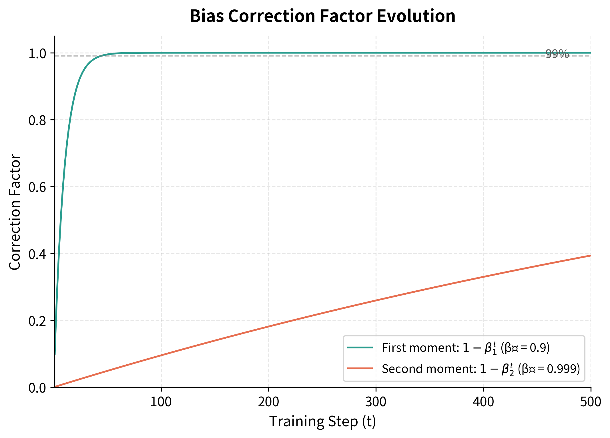
This visualization reveals an important asymmetry. The first moment correction converges rapidly because $\beta_1 = 0.9$ means 90% retention per step. After just 22 steps, $(1 - 0.9^{22}) > 0.9$, so the correction is already small. The second moment correction with $\beta_2 = 0.999$ takes much longer: we need nearly 700 steps before $(1 - 0.999^{700}) > 0.5$. This slower convergence is intentional, as it provides a more stable variance estimate by incorporating more history.

Step 5: Update weights with decoupled decay. Finally, we perform both the Adam update and weight decay in a single step:

This equation combines two independent forces acting on each weight:

1. The adaptive gradient step $\frac{\hat{m}_t}{\sqrt{\hat{v}_t} + \epsilon}$: This is pure Adam. The bias-corrected momentum $\hat{m}_t$ tells us which direction to move, while dividing by $\sqrt{\hat{v}_t}$ scales the step size inversely with gradient magnitude.

2. The decoupled weight decay term $\lambda w_t$: This shrinks weights toward zero at rate $\lambda$, applied directly without any scaling by gradient history.

The small constant $\epsilon$ (typically $10^{-8}$) prevents division by zero when $\hat{v}_t$ is very small.

An equivalent formulation makes the decay mechanism more explicit:

Here you can see weight decay as a multiplicative factor: before applying the gradient update, we shrink all weights by $(1 - \eta \lambda)$. For typical values like $\eta = 10^{-3}$ and $\lambda = 0.01$, this factor equals 0.99999. Each individual step produces barely perceptible decay, but over thousands of steps, the cumulative effect is substantial.

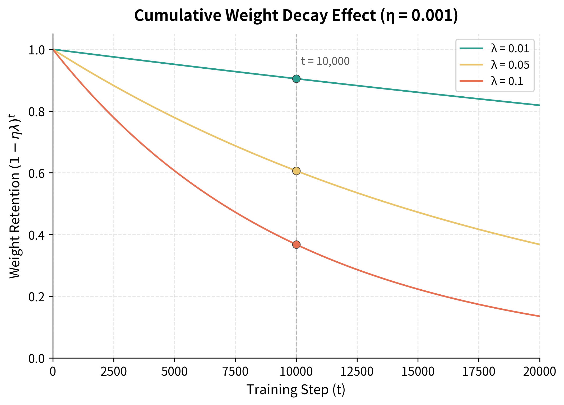
This plot shows why weight decay values in the range 0.01 to 0.1 are typical. With $\lambda = 0.01$, weights decay slowly enough that important features are preserved, but unnecessary weights still shrink over the course of training. With $\lambda = 0.1$, the decay is aggressive, which can help with heavily overparameterized models but may hurt performance if set too high. The key insight is that gradients continually push back against this decay for weights that are important for minimizing the loss, creating a natural equilibrium.

The weight decay coefficient $\lambda$ requires careful tuning. Unlike learning rate, which has relatively universal starting points, optimal weight decay varies significantly across architectures and datasets.

For transformer models, weight decay values typically fall between 0.01 and 0.1:

• BERT and variants: Originally trained with $\lambda = 0.01$
• GPT-2 and GPT-3: Used $\lambda = 0.1$
• Vision Transformers: Often use $\lambda = 0.05$ to $0.3$
• ResNets with AdamW: Commonly use $\lambda = 0.01$ to $0.05$

Larger models often benefit from stronger regularization. This makes intuitive sense: with more parameters comes more capacity for overfitting.

Weight decay and learning rate interact because the effective decay per step is $\eta \lambda$. When tuning learning rate with a learning rate schedule, you have two choices:

• Keep $\lambda$ fixed: The effective decay decreases as learning rate decays. This is the standard approach and generally works well.
• Scale $\lambda$ with learning rate: Maintains constant effective decay throughout training. Some practitioners prefer this for very long training runs.

Most frameworks use fixed $\lambda$, and the decreasing effective decay late in training can actually help the model settle into sharper minima.

Not all parameters should receive weight decay. The standard practice is to exclude:

• Bias terms: These don't contribute to overfitting in the same way as weights
• Layer normalization parameters: Both scale ($\gamma$) and shift ($\beta$) parameters
• Embedding layers: Sometimes excluded, though practices vary

Let's see how to implement this in PyTorch:

The weight matrices contain most of the parameters and receive regularization, while biases and normalization parameters remain unregularized. This split is now standard practice in transformer training.

The best way to internalize an algorithm is to implement it yourself. Let's build AdamW from scratch using only NumPy, translating each mathematical step into code. This exercise will reveal how elegantly simple the algorithm is once you understand the underlying concepts.

Our implementation needs to maintain state across optimization steps: the moment estimates $m$ and $v$ for each parameter, plus a step counter $t$ for bias correction. We'll structure this as a class that mirrors how production optimizers work.

Notice how the implementation follows our five-step algorithm exactly. The constructor initializes moment estimates to zero (creating the bias that we later correct). The step method increments the counter, updates both moments using exponential moving averages, applies bias correction, and finally performs the decoupled update.

The critical line is the final update: m_hat / (np.sqrt(v_hat) + self.eps) + self.weight_decay * param. We add the weight decay term after computing the adaptive gradient step, ensuring that decay operates independently of gradient history. If we had instead modified the gradient before computing moments (as L2 regularization does), the decay would be dampened by the adaptive mechanism.

Let's verify our implementation works correctly on a problem where we can visualize the optimization trajectory. We'll minimize $f(x, y) = x^2 + 10y^2$, an elongated bowl that's a classic test for optimizers. The steeper curvature along $y$ means gradients are larger in that direction, which tests whether our adaptive learning rates work correctly.

Our implementation successfully drives both coordinates toward zero, with the loss decreasing by several orders of magnitude. The $y$ coordinate converges faster initially because its gradients are larger (the derivative $\frac{\partial f}{\partial y} = 20y$ is 10 times the derivative with respect to $x$). However, Adam's adaptive mechanism compensates: larger gradients lead to larger second moment estimates, which reduce the effective learning rate along $y$. This balancing act is precisely what makes Adam so effective on problems with different scales across dimensions.

The weight decay provides an additional gentle pull toward the origin. Even if the loss function had a minimum elsewhere, weight decay would bias the solution toward smaller weights, which is exactly the regularization behavior we want in neural network training.

In practice, you'll use PyTorch's built-in AdamW implementation, which is highly optimized and supports features like gradient scaling for mixed-precision training:

The loss decreases steadily as AdamW optimizes the network. In real applications, you would also track validation loss to monitor generalization.

Theory tells us that L2 regularization and weight decay should behave differently with Adam, but seeing is believing. Let's run both approaches side by side on our elongated bowl problem and plot their optimization trajectories. This visualization will make the abstract mathematical difference concrete.

We'll implement Adam with L2 regularization (where $\lambda w$ is added to the gradient before entering the moment calculations) alongside our AdamW implementation (where weight decay is applied after the adaptive update). Both start from the same point and use identical hyperparameters:

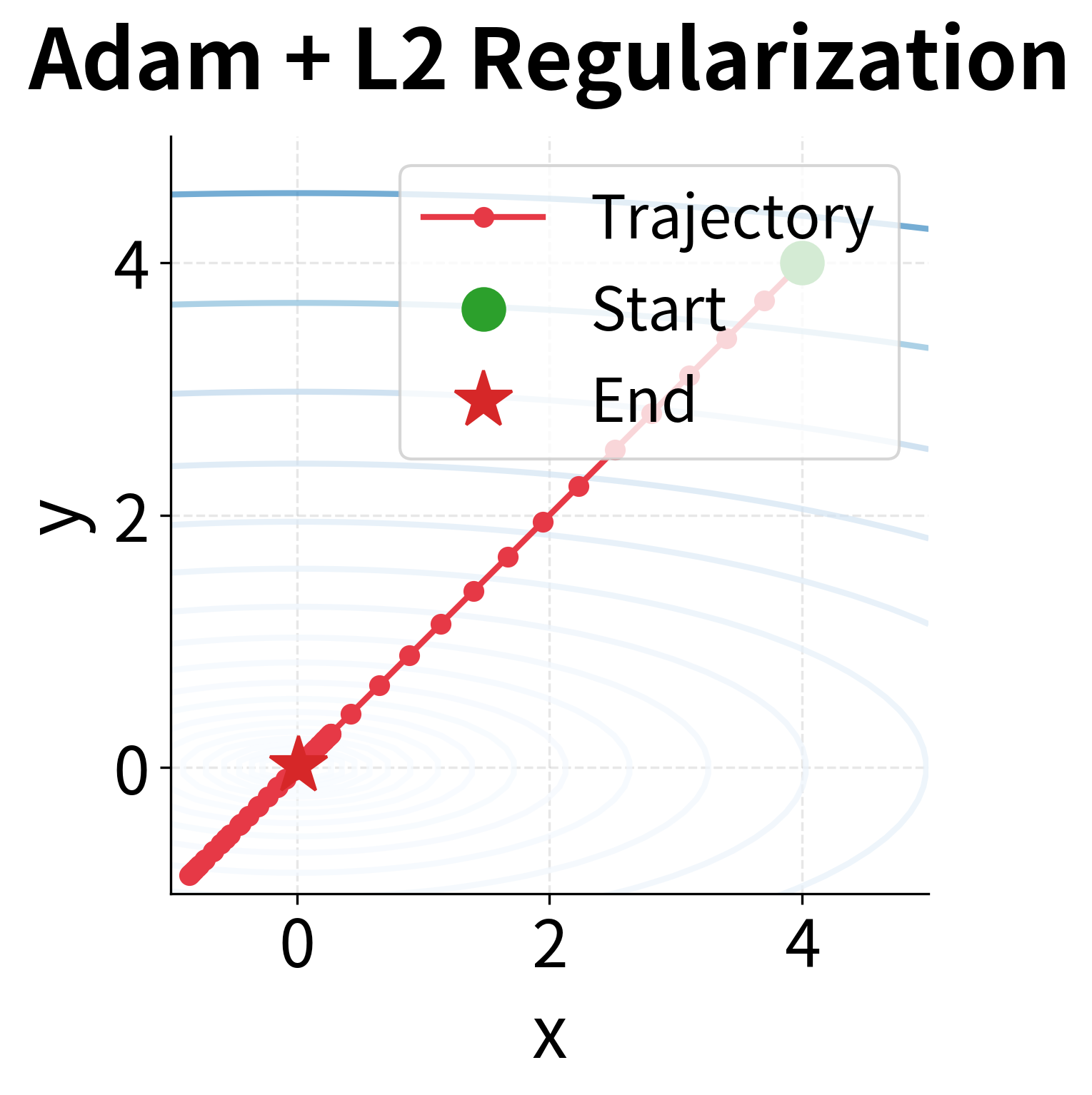
The trajectories tell a striking story. Adam with L2 regularization follows a more wandering path, particularly in the early stages when the regularization gradients are large. Look carefully at the $y$-axis convergence: because the gradient along $y$ is larger (due to the steeper curvature), the L2 term $\lambda w$ gets scaled down more aggressively by Adam's adaptive mechanism. The regularization signal is weakest precisely where weights are largest.

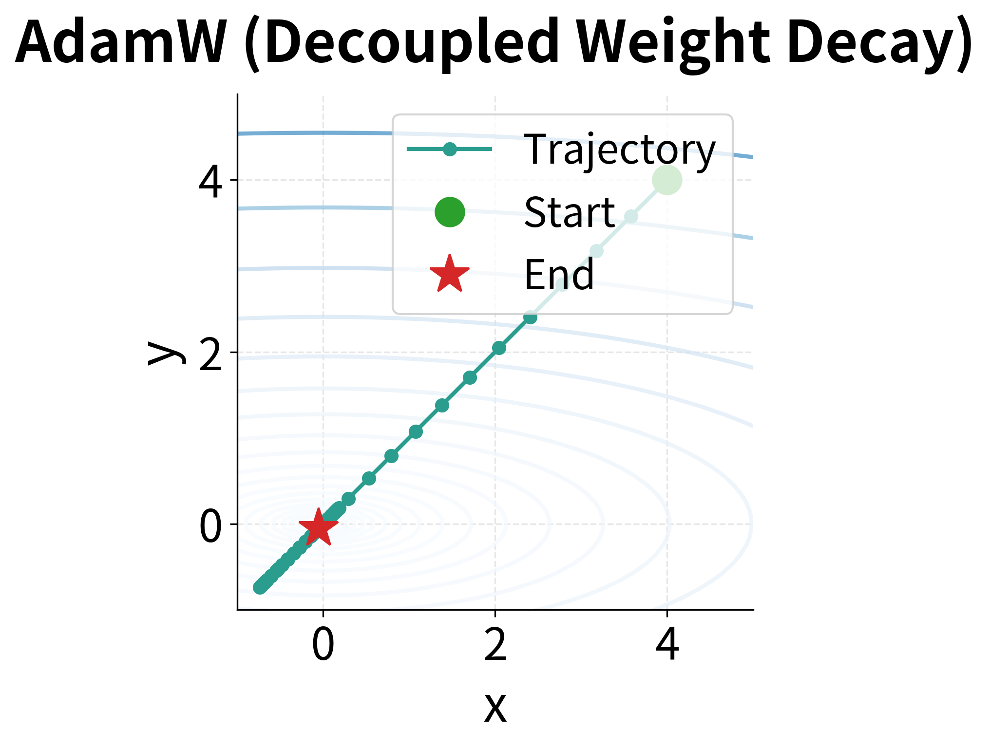
AdamW, by contrast, produces a cleaner, more direct trajectory. The decoupled weight decay shrinks weights uniformly regardless of gradient history. Along the $y$-axis, where curvature is steep, the adaptive learning rate still reduces step size, but weight decay continues operating at full strength. This is exactly what we want: efficient optimization (via adaptation) combined with consistent regularization (via decoupling).

In neural network training, this difference compounds over millions of steps across millions of parameters. The improved regularization consistency translates directly into better generalization, which is why AdamW has become the standard for training large models.

AdamW has become the de facto standard for training transformers and large language models. This wasn't always the case: early language models like the original GPT were trained with Adam plus L2 regularization. The shift to AdamW happened as researchers noticed consistent improvements in generalization.

Several factors make AdamW particularly well-suited for transformers:

• Consistent regularization: Transformers have parameters with vastly different gradient scales. Self-attention weights, feedforward layers, and embeddings all behave differently during training. AdamW's decoupled decay provides uniform regularization regardless of these gradient patterns.

• Better with large batch sizes: Modern language models use large batches for efficiency. AdamW's proper weight decay helps prevent the generalization gap that can emerge with large-batch training.

• Stable with learning rate warmup: Transformer training typically uses linear warmup followed by decay. AdamW behaves predictably throughout this schedule because weight decay doesn't interact with the adaptive learning rate mechanism.

A typical configuration for training transformer models with AdamW includes:

• Learning rate: 1e-4 to 1e-3, with linear warmup over 1-10% of training
• Weight decay: 0.01 to 0.1
• Betas: (0.9, 0.999) or (0.9, 0.98) for stability
• Epsilon: 1e-8 or 1e-6 for numerical stability

Let's see this configuration in action:

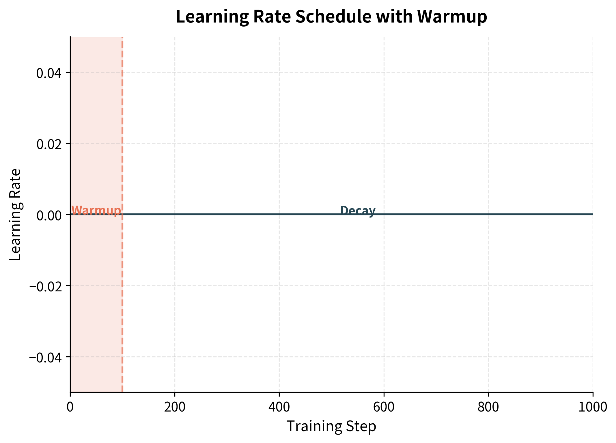
The warmup phase gradually increases the learning rate, preventing early instability when the model's gradients are large and poorly calibrated. Early in training, weights are randomly initialized and gradients can be very large and erratic. Starting with a small learning rate allows the optimizer to build up accurate moment estimates before taking larger steps. After warmup, the learning rate decays linearly, allowing the model to settle into a good minimum with increasingly precise updates.

Let's run a controlled experiment comparing Adam with L2 regularization against AdamW on a classification task:

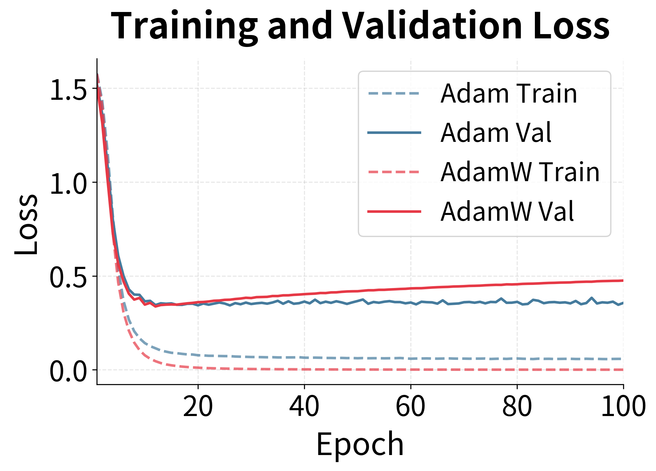
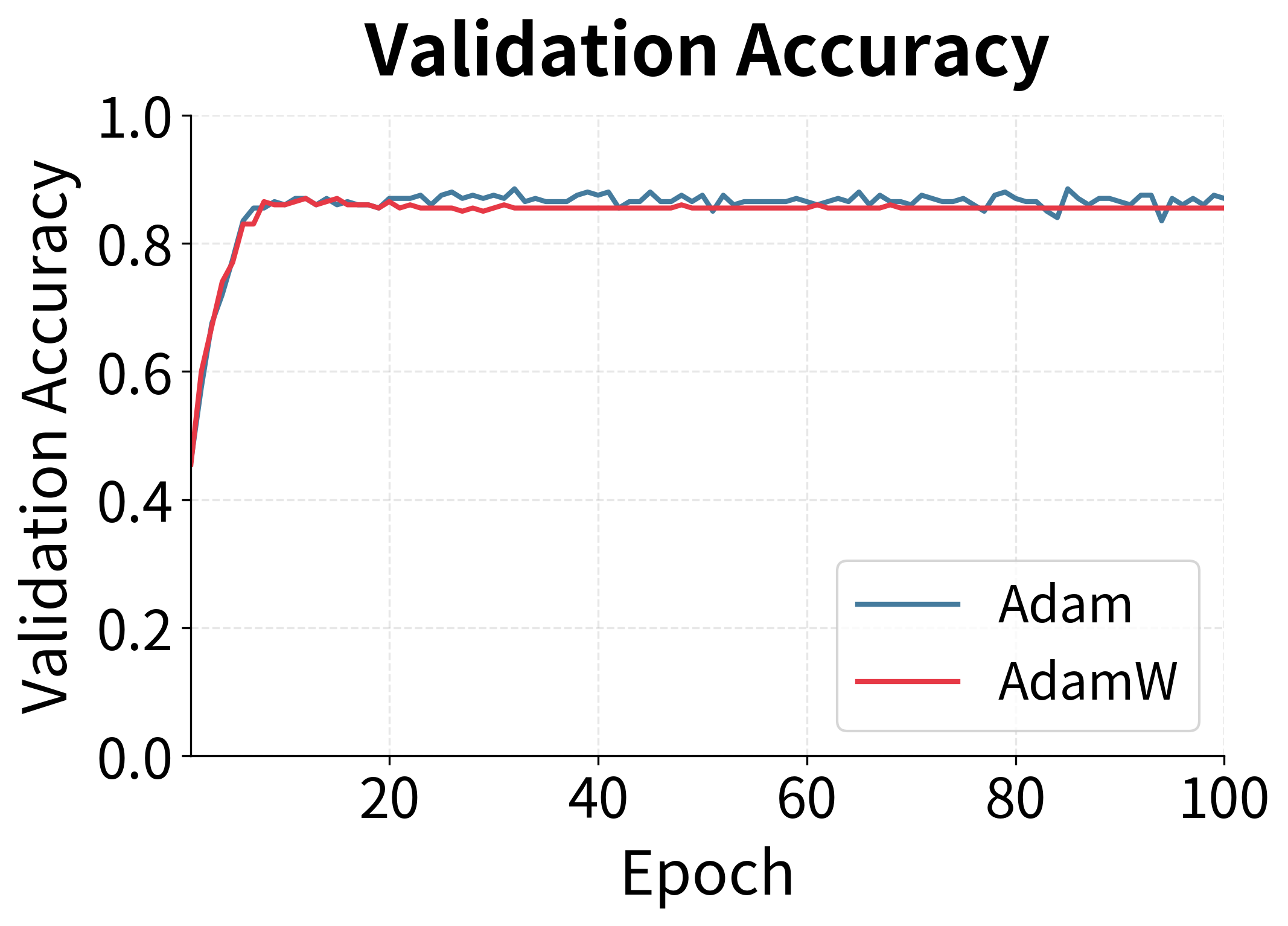
The experiment reveals AdamW's advantage in generalization. While both optimizers reduce training loss similarly, AdamW achieves better validation performance. The gap becomes more pronounced with longer training, as the proper weight decay in AdamW continues to prevent overfitting while L2 regularization's effectiveness diminishes due to Adam's adaptive mechanism.

AdamW is not a universal solution. Understanding its limitations helps you make informed choices about when to use it and how to configure it effectively.

Like Adam, AdamW maintains two moment estimates per parameter, increasing the memory required for optimizer state compared to SGD with momentum. For a model with $n$ parameters, AdamW stores:

• The parameters themselves: $n$ floats
• First moment estimates $m$: $n$ floats
• Second moment estimates $v$: $n$ floats

This totals $3n$ floats, compared to $2n$ for SGD with momentum. For a 7-billion parameter model using 32-bit floats, this means approximately 84 GB for optimizer state alone. Techniques like gradient checkpointing, mixed-precision training (which stores moments in lower precision), and optimizer state offloading help mitigate this cost, but the overhead remains a consideration when memory is constrained.

While AdamW is more robust than Adam with L2 regularization, it still requires careful hyperparameter tuning. The weight decay coefficient interacts with learning rate, batch size, and training duration. What works for BERT may not work for GPT, and vice versa. Start with established recipes from similar architectures and adjust based on validation performance. Pay particular attention to the learning rate schedule: AdamW works best with warmup followed by gradual decay, and the warmup length matters more than with other optimizers.

For some applications, other optimizers may be preferable:

• SGD with momentum: Often achieves better final generalization on vision tasks, despite slower convergence
• Adafactor: Reduces memory by factorizing the second moment estimate, useful for very large models
• LAMB: Designed specifically for large-batch training, can enable faster distributed training

AdamW remains the safe default for language models and transformers, but don't hesitate to experiment with alternatives if your specific application has different constraints.

AdamW fixes a fundamental problem with how Adam handles regularization. The key insights are:

• L2 regularization and weight decay are equivalent for SGD but not for Adam. Adam's adaptive learning rates dampen the L2 regularization signal, reducing its effectiveness precisely where it should be strongest.

• AdamW decouples weight decay from the gradient update. By applying weight decay directly to the parameters rather than through the gradient path, AdamW maintains consistent regularization regardless of gradient history.

• The AdamW update adds an explicit decay term. The formula $w_{t+1} = w_t - \eta(\hat{m}_t / \sqrt{\hat{v}_t} + \lambda w_t)$ separates the gradient-based learning from the regularization, where the decay $\lambda w_t$ is not scaled by the adaptive factor.

• Not all parameters should receive weight decay. Standard practice excludes biases, layer normalization parameters, and sometimes embeddings from weight decay.

• AdamW is the default optimizer for transformers. Its consistent regularization, stability with learning rate schedules, and robustness across different gradient scales make it ideal for modern language models.

The difference between Adam and AdamW may seem subtle, but it has real impact on model generalization. When training neural networks, especially transformers and language models, AdamW should be your starting point.

When configuring AdamW for your models, the following parameters have the most significant impact on training:

• lr (learning rate): Controls the step size for parameter updates. Typical values range from 1e-5 to 1e-3. For transformers, start with 1e-4 and adjust based on validation loss. Use warmup to prevent early training instability.

• weight_decay: The decoupled regularization coefficient. Values between 0.01 and 0.1 work well for most transformer architectures. Larger models often benefit from stronger decay. This parameter should be excluded for biases and layer normalization parameters.

• betas: A tuple (β₁, β₂) controlling the exponential decay rates for the moment estimates. The default (0.9, 0.999) works well in most cases. For transformers, some practitioners use (0.9, 0.98) for slightly faster adaptation to gradient changes.

• eps: A small constant added for numerical stability. The default 1e-8 works for most cases, but 1e-6 can help with mixed-precision training where smaller values may cause overflow.

• amsgrad: When True, uses the maximum of past squared gradients rather than the exponential moving average. This can help with convergence in some cases but is rarely needed in practice.

Ready to test your understanding? Take this quick quiz to reinforce what you've learned about AdamW and decoupled weight decay.