Multilayer Perceptrons: Architecture, Forward Pass & Implementation

In the previous chapters, we explored linear classifiers and activation functions as separate building blocks. Linear classifiers can find decision boundaries, but only straight ones. Activation functions introduce non-linearity, but a single neuron with an activation still has limited representational power. The breakthrough comes when we stack these components together into layers, creating what we call a multilayer perceptron (MLP).

MLPs are the workhorses of deep learning. They can approximate virtually any function given enough neurons and proper training. From sentiment analysis to language modeling, understanding MLPs is essential because they form the building blocks of more complex architectures like transformers. This chapter shows you how to construct, understand, and implement MLPs from the ground up.

A single neuron computes a weighted sum of its inputs, adds a bias, and passes the result through an activation function. Given an input vector $\mathbf{x} = [x_1, x_2, \ldots, x_n]$ with $n$ features, the neuron computes:

where:

• $\mathbf{x}$: the input vector containing $n$ features
• $\mathbf{w}$: the weight vector, where each $w_i$ controls how much input $x_i$ influences the output
• $\mathbf{w}^\top \mathbf{x}$: the dot product $\sum_{i=1}^{n} w_i x_i$, computing a weighted sum of inputs
• $b$: the bias term, which shifts the decision boundary
• $\sigma$: the activation function (e.g., ReLU, sigmoid), which introduces non-linearity
• $y$: the scalar output of the neuron

This single neuron can learn a linear decision boundary (made non-linear by $\sigma$), but it cannot solve problems requiring more complex boundaries.

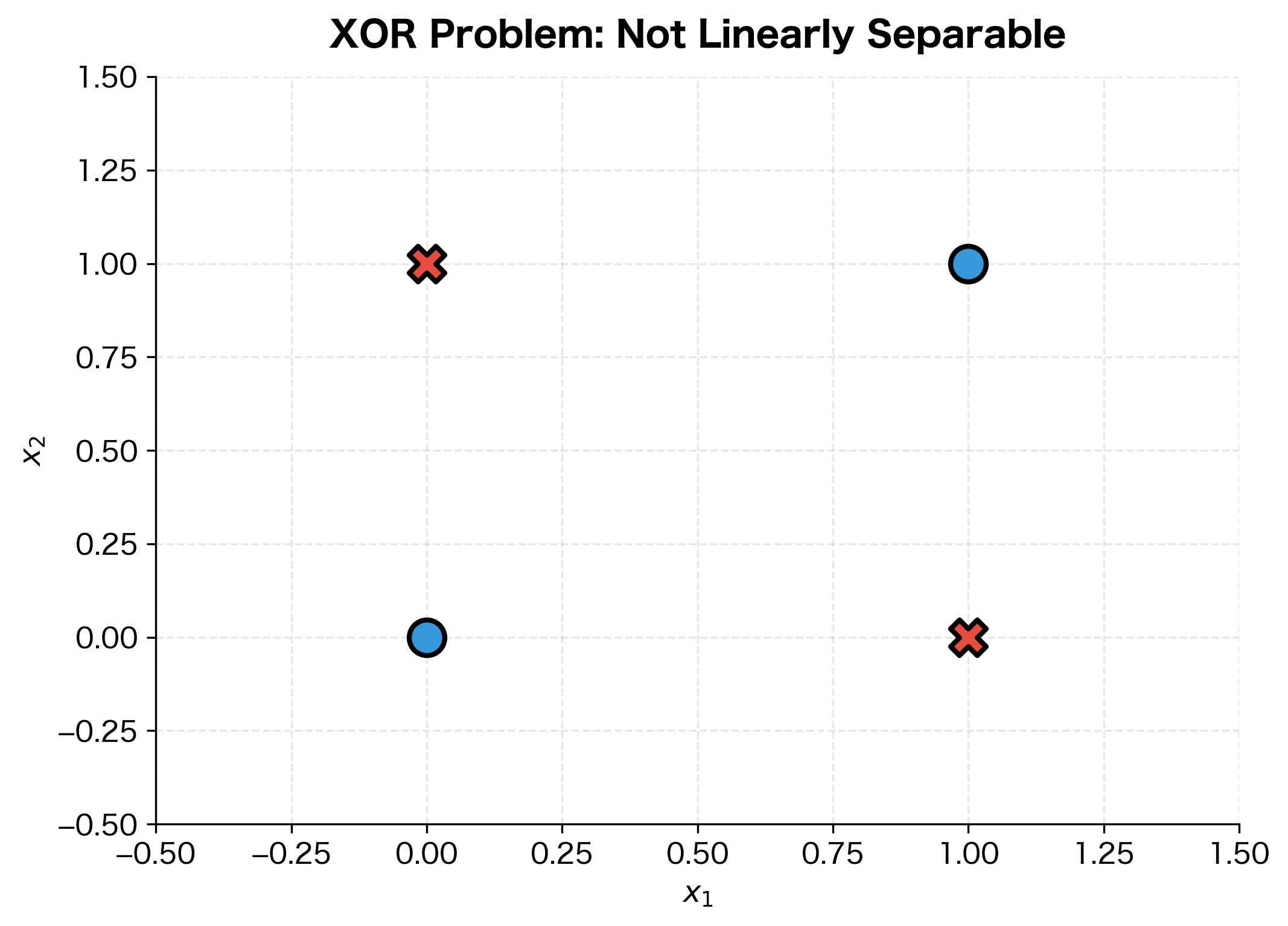
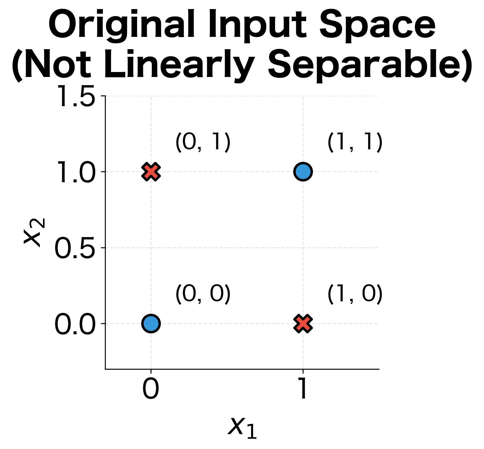
Consider the classic XOR problem: given two binary inputs, output 1 if exactly one input is 1, and 0 otherwise. No single linear boundary can separate the positive from negative examples. But with a hidden layer, we can first transform the inputs into a new representation where the classes become linearly separable.

The magic happens when we add a hidden layer. Each hidden neuron learns to detect a different feature or pattern in the input. The output layer then combines these learned features to make the final prediction.

To see this in action, let's manually construct a hidden layer that solves XOR and visualize how it transforms the input space:

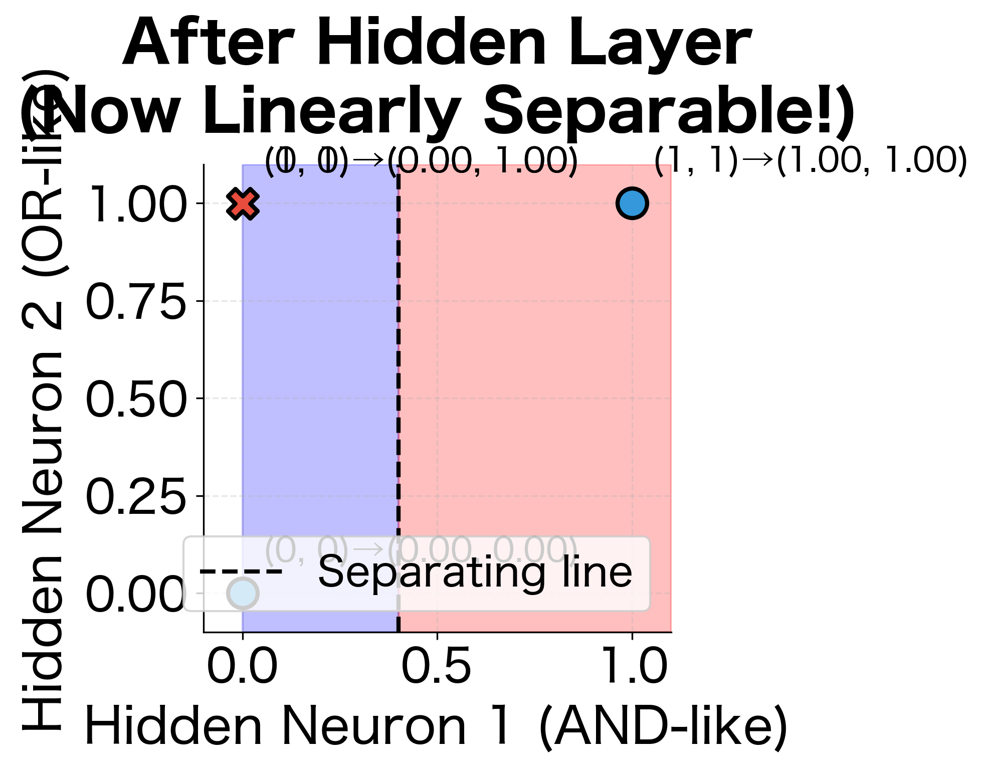
The hidden layer has transformed the input space so that a simple linear classifier can now separate the classes. The first hidden neuron activates only when both inputs are high (AND-like behavior), while the second activates when either input is high (OR-like behavior). In this new coordinate system, the XOR pattern becomes trivially separable.

An MLP consists of an input layer, one or more hidden layers, and an output layer. We describe the architecture by the number of units in each layer. For example, a network with 4 inputs, two hidden layers of 8 and 4 units, and 2 outputs would be written as 4-8-4-2.

Let's establish notation that will serve us throughout this chapter and beyond:

• $L$: Total number of layers (excluding input)
• $n^{[l]}$: Number of neurons in layer $l$
• $\mathbf{W}^{[l]}$: Weight matrix for layer $l$, with shape $(n^{[l]}, n^{[l-1]})$
• $\mathbf{b}^{[l]}$: Bias vector for layer $l$, with shape $(n^{[l]}, 1)$
• $\mathbf{z}^{[l]}$: Pre-activation values at layer $l$
• $\mathbf{a}^{[l]}$: Activations (post-activation values) at layer $l$
• $\mathbf{a}^{[0]} = \mathbf{x}$: The input is treated as the activation of layer 0

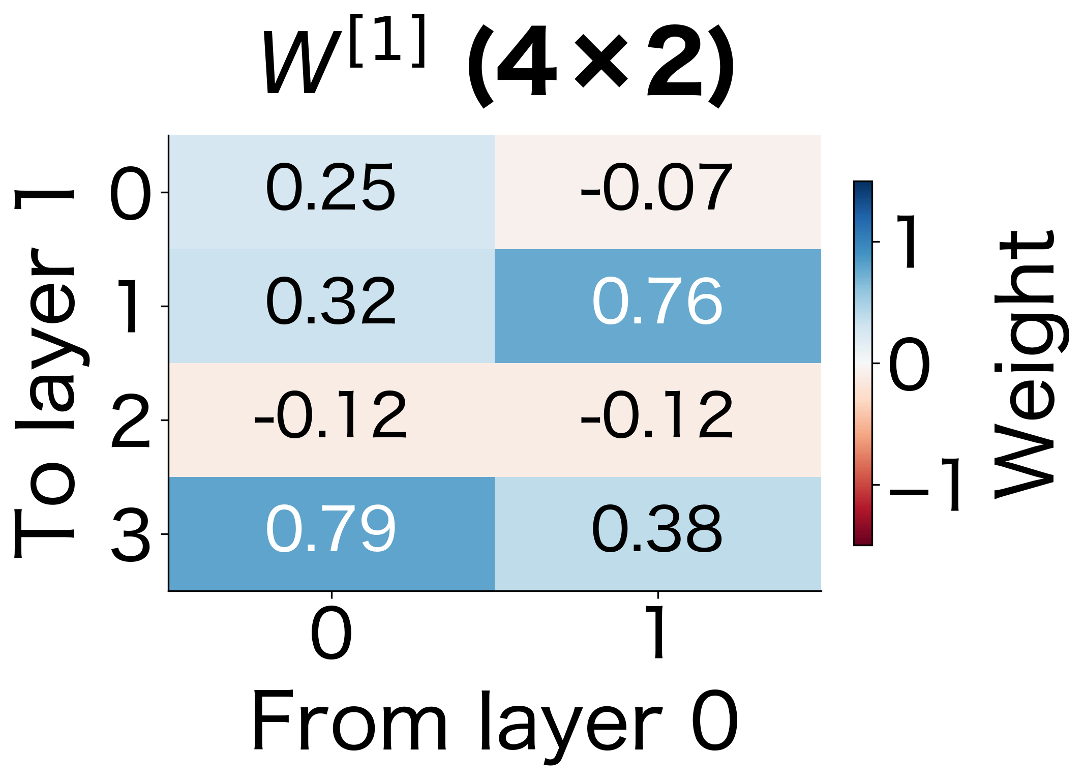
The weight matrix $\mathbf{W}^{[l]}$ connects layer $l-1$ to layer $l$. Each row of $\mathbf{W}^{[l]}$ contains the weights for one neuron in layer $l$. The element $W^{[l]}_{ij}$ represents the weight connecting neuron $j$ in layer $l-1$ to neuron $i$ in layer $l$.

This 3-layer network has a modest parameter count, but the numbers grow quickly. Let's visualize what these weight matrices actually look like:

The weight matrices grow with the product of consecutive layer sizes. A layer connecting 512 neurons to 256 neurons requires $512 \times 256 = 131,072$ parameters just for the weights, plus 256 bias terms. This rapid growth in parameters is why network architecture design requires careful consideration.

With our notation established, we can now understand how an MLP transforms an input into an output. This process, called the forward pass, is the heart of neural network computation. Think of it as a pipeline: data flows in one direction, from input through hidden layers to output, with each layer transforming the representation along the way.

At each layer, the network performs two distinct operations that work together to create expressive transformations:

Step 1: Linear Transformation. First, we compute a weighted combination of inputs from the previous layer. This is where the learnable parameters (weights and biases) come into play:

The weight matrix $\mathbf{W}^{[l]}$ determines how strongly each input neuron influences each output neuron. The bias vector $\mathbf{b}^{[l]}$ shifts the output, allowing neurons to activate even when inputs are zero. Together, they define a linear transformation that can rotate, scale, and translate the input space.

Step 2: Non-linear Activation. Next, we apply an activation function element-wise to introduce non-linearity:

This step is crucial. Without activation functions, stacking multiple linear transformations would collapse into a single linear transformation, no matter how many layers we add. The activation function $\sigma$ bends and warps the space, allowing the network to model complex, non-linear relationships.

For a network with $L$ layers, the forward pass chains these two-step computations together. Starting with the input $\mathbf{x}$ (which we treat as $\mathbf{a}^{[0]}$), we propagate through each layer:

where:

• $\mathbf{z}^{[l]}$: the pre-activation vector at layer $l$, the raw output of the linear transformation before any non-linearity is applied
• $\mathbf{a}^{[l]}$: the activation vector at layer $l$, the output after applying the activation function, which becomes input to the next layer
• $\mathbf{W}^{[l]}$: the weight matrix connecting layer $l-1$ to layer $l$, containing $n^{[l]} \times n^{[l-1]}$ learnable parameters
• $\mathbf{b}^{[l]}$: the bias vector for layer $l$, containing $n^{[l]}$ learnable parameters
• $\sigma$: the activation function applied element-wise (e.g., ReLU, sigmoid, tanh)
• $\hat{\mathbf{y}}$: the network's final output, our prediction

The power of this layered structure comes from composition. Each layer learns to detect increasingly abstract features:

1. Early layers learn simple patterns directly from the input (edges, basic shapes, common word fragments)
2. Middle layers combine these simple patterns into more complex features (textures, object parts, phrases)
3. Later layers assemble these features into high-level concepts (objects, categories, meanings)

The output layer typically uses a different activation than hidden layers, chosen based on the task. For binary classification, sigmoid squashes output to $(0, 1)$ for probability interpretation. For multiclass classification, softmax produces a probability distribution across classes. For regression, we often use no activation (identity function) to allow unbounded predictions.

Let's translate these mathematical concepts into code. We'll build a forward pass function from scratch using NumPy to see exactly how the computation flows.

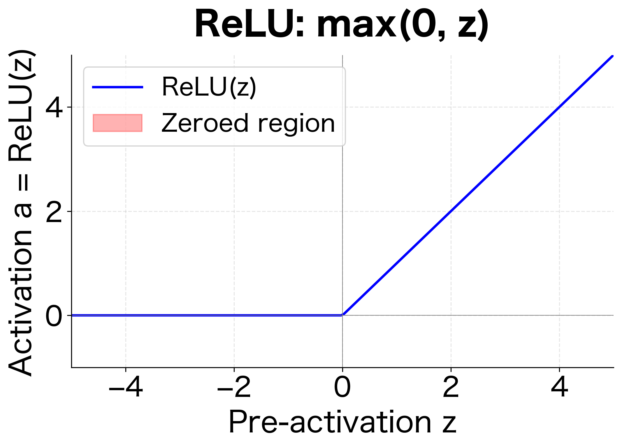
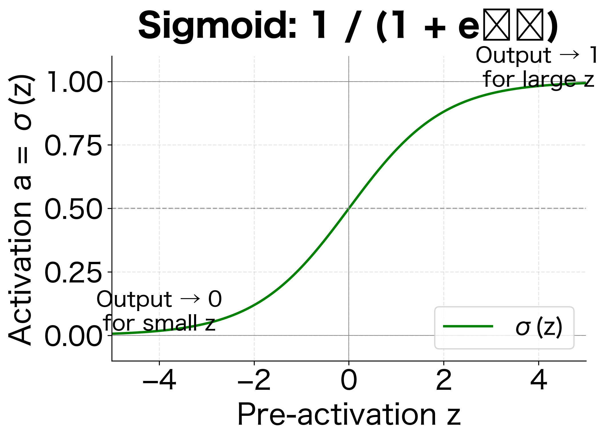
First, we define our activation functions. ReLU (Rectified Linear Unit) is the most common choice for hidden layers because it's simple, computationally efficient, and helps avoid the vanishing gradient problem. Sigmoid is useful for the output layer in binary classification, where we need probabilities between 0 and 1.

Now we implement the forward pass itself. The function iterates through each layer, applying the two-step computation we described: linear transformation followed by activation.

To solidify our understanding, let's trace through the forward pass with actual numbers. We'll use the 2-4-3-1 network we defined earlier and pass a single input through it.

The forward pass transforms our 2D input through three layers, ultimately producing a single scalar output. Several key observations emerge from this trace:

1. ReLU's effect on hidden layers: Notice how negative pre-activation values become zero after ReLU. This sparsity (many zeros) is actually beneficial, making the network more computationally efficient and helping prevent overfitting.

2. Dimensional changes: The representation changes size at each layer, from 2 dimensions (input) to 4, then 3, then finally 1 (output). The network progressively compresses information toward the final prediction.

3. Sigmoid's bounded output: The final layer's sigmoid activation squashes the output to a probability between 0 and 1, suitable for binary classification.

4. Composition creates complexity: Although each individual step is simple (matrix multiply, add bias, apply activation), the composition of many such steps creates a highly non-linear function capable of modeling complex patterns.

The forward pass we implemented processes one example at a time, but this is inefficient in practice. Modern hardware, especially GPUs, is designed for parallel computation. By processing multiple examples simultaneously, we can achieve dramatic speedups.

The key insight is that we can stack multiple input vectors into a matrix, where each column represents one example. Instead of looping through examples one by one, we perform a single matrix multiplication that processes all examples at once.

For a batch of $m$ examples, the input becomes a matrix $\mathbf{X}$ of shape $(n^{[0]}, m)$, where each column represents one example. The forward pass equations generalize elegantly to matrix form:

where:

• $\mathbf{A}^{[l-1]}$: the activation matrix from the previous layer, with shape $(n^{[l-1]}, m)$
• $\mathbf{W}^{[l]}$: the weight matrix with shape $(n^{[l]}, n^{[l-1]})$
• $\mathbf{Z}^{[l]}$: the pre-activation matrix with shape $(n^{[l]}, m)$
• $\mathbf{b}^{[l]}$: the bias vector with shape $(n^{[l]}, 1)$, broadcast across all $m$ columns
• $m$: the batch size (number of examples processed simultaneously)

The matrix multiplication $\mathbf{W}^{[l]} \mathbf{A}^{[l-1]}$ computes the linear transformation for all examples at once. The bias vector $\mathbf{b}^{[l]}$ is broadcast (replicated) across all $m$ columns, adding the same bias to each example. The activation function is then applied element-wise to produce $\mathbf{A}^{[l]}$.

All five examples are processed in a single matrix operation, producing five outputs simultaneously. The varying output values reflect the different input features for each example. Batch processing is not just about efficiency. It also provides more stable gradient estimates during training, as we will see in the backpropagation chapter.

One of the most remarkable properties of MLPs is their ability to approximate any continuous function. The Universal Approximation Theorem states that a feedforward network with a single hidden layer containing a finite number of neurons can approximate any continuous function on a compact subset of $\mathbb{R}^n$, given appropriate weights.

The theorem tells us that MLPs are expressive enough to represent complex functions. However, it says nothing about:

• How many neurons are needed (could be exponentially many)
• Whether training will find good weights
• How well the network will generalize to new data

In practice, we find that deeper networks (more layers) often work better than wider networks (more neurons per layer) for the same total number of parameters. Depth enables hierarchical feature learning, where early layers detect simple patterns and later layers combine them into complex concepts.

The shallow network actually has the most parameters despite having only one hidden layer. The deeper networks distribute their capacity across more layers with fewer neurons each. Let's visualize this trade-off:

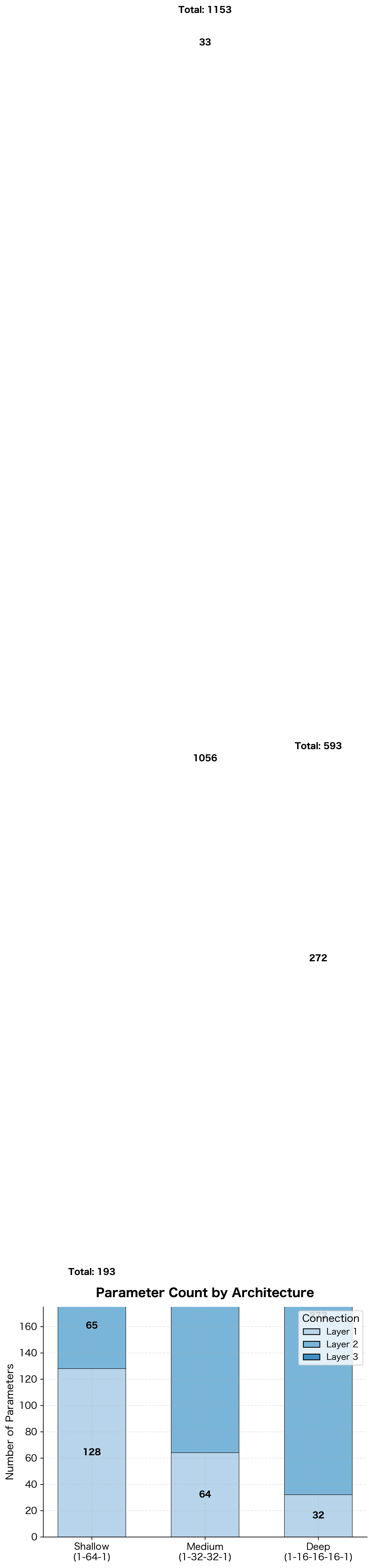
This trade-off matters: deeper networks can represent more complex compositional functions. Think of it like building with LEGO: a few large blocks can cover area, but many small blocks arranged hierarchically can create intricate structures.

Classification is one of the most common tasks for MLPs. The network takes features as input and produces probabilities for each class. For binary classification, we use a single output neuron with sigmoid activation. For multiclass, we use multiple output neurons with softmax activation.

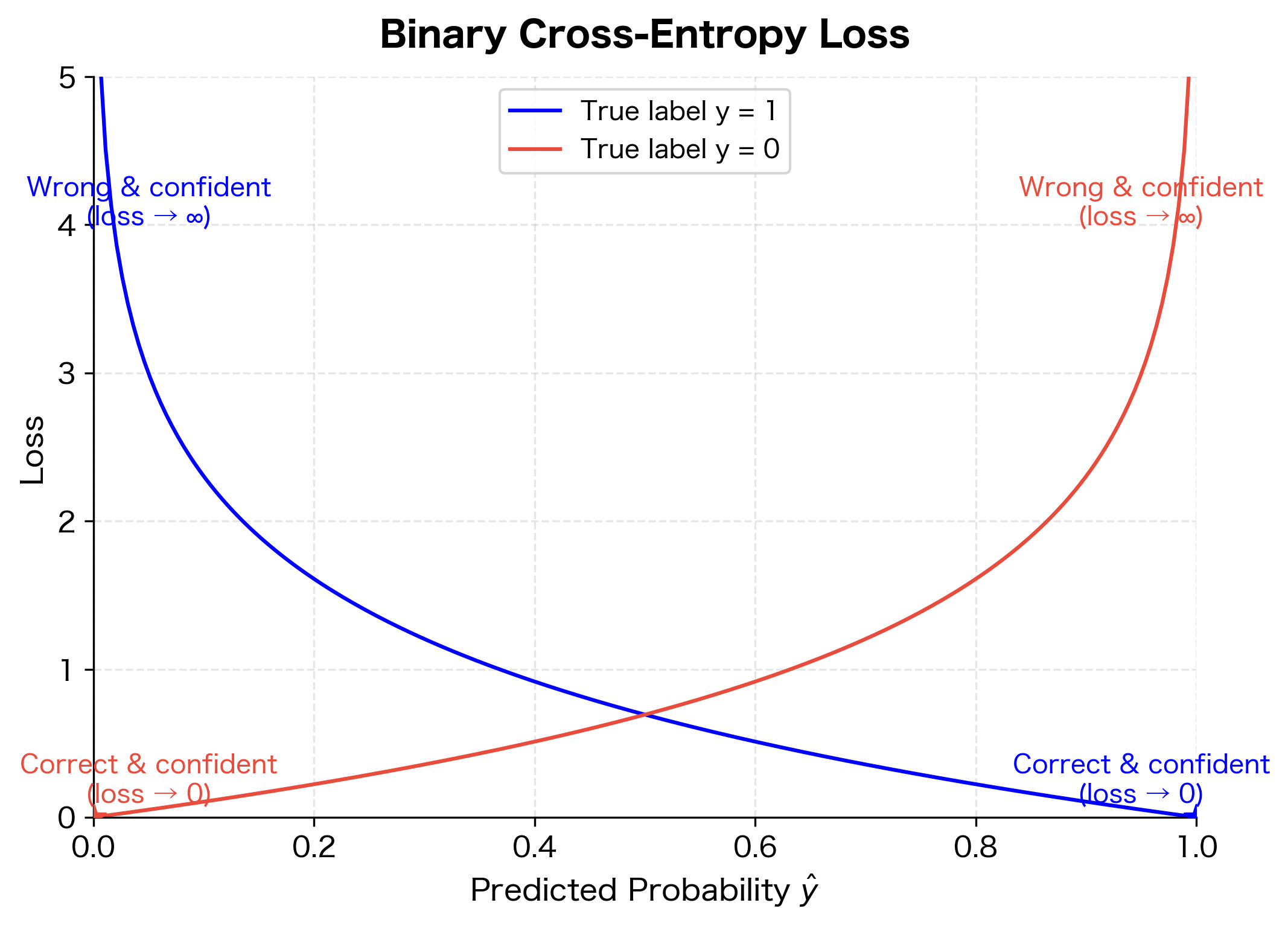
In binary classification, the output $\hat{y} \in (0, 1)$ represents the probability that the input belongs to class 1. We train the network by minimizing the binary cross-entropy loss, which measures how well the predicted probabilities match the true labels:

where:

• $m$: the number of training examples in the batch
• $y^{(i)}$: the true label for example $i$ (either 0 or 1)
• $\hat{y}^{(i)}$: the predicted probability that example $i$ belongs to class 1
• $\log$: the natural logarithm

This loss function has an intuitive interpretation. When the true label is $y^{(i)} = 1$, only the first term $-\log(\hat{y}^{(i)})$ is active, which penalizes low predicted probabilities. When $y^{(i)} = 0$, only the second term $-\log(1 - \hat{y}^{(i)})$ is active, penalizing high predicted probabilities. The loss approaches zero when predictions are confident and correct, and grows large when predictions are wrong.

Let's build a complete binary classifier using PyTorch:

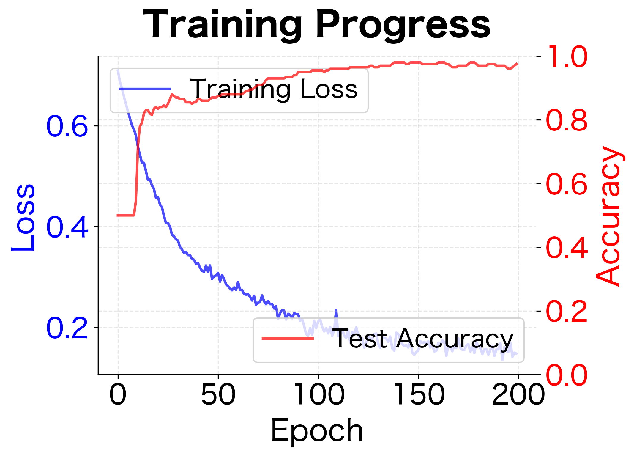
The model achieves strong test accuracy after 200 epochs of training. The significant reduction in loss from start to finish indicates successful learning. A test accuracy above 85% on the two moons dataset suggests the network has learned the non-linear decision boundary effectively.

Let's visualize the decision boundary learned by our classifier:

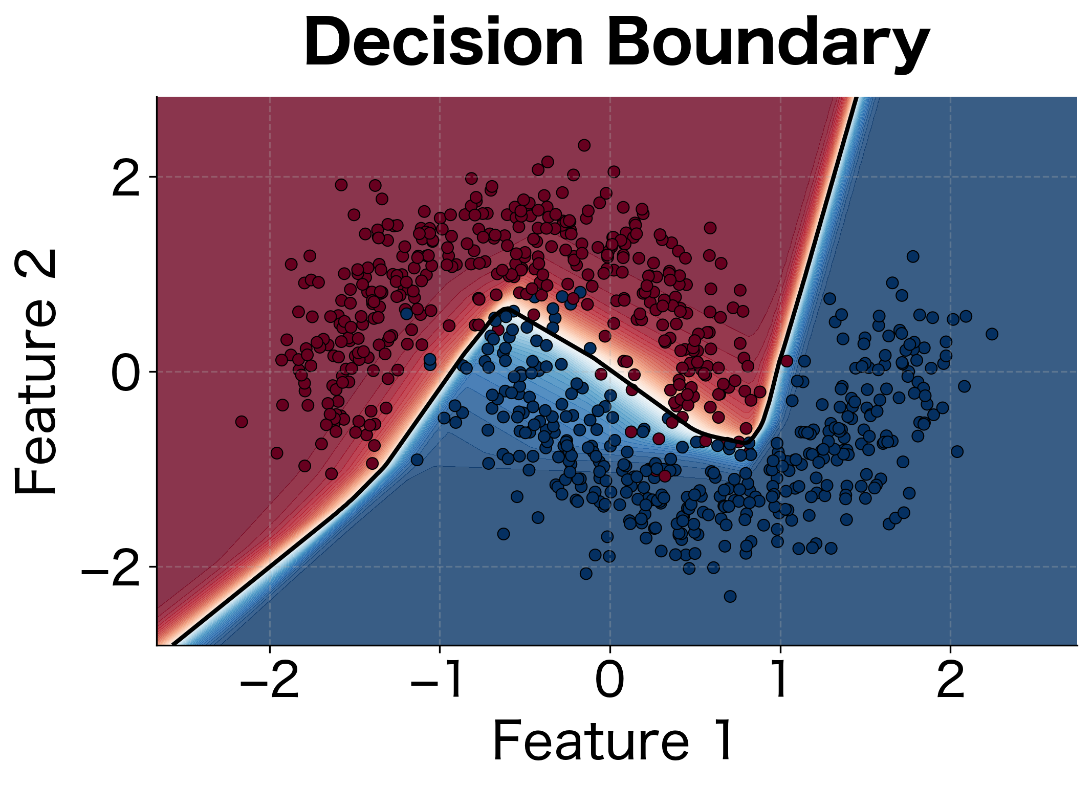
The MLP learns a curved decision boundary that cleanly separates the two moon-shaped clusters. A linear classifier would fail miserably on this task, but the hidden layer transforms the input into a representation where the classes become separable.

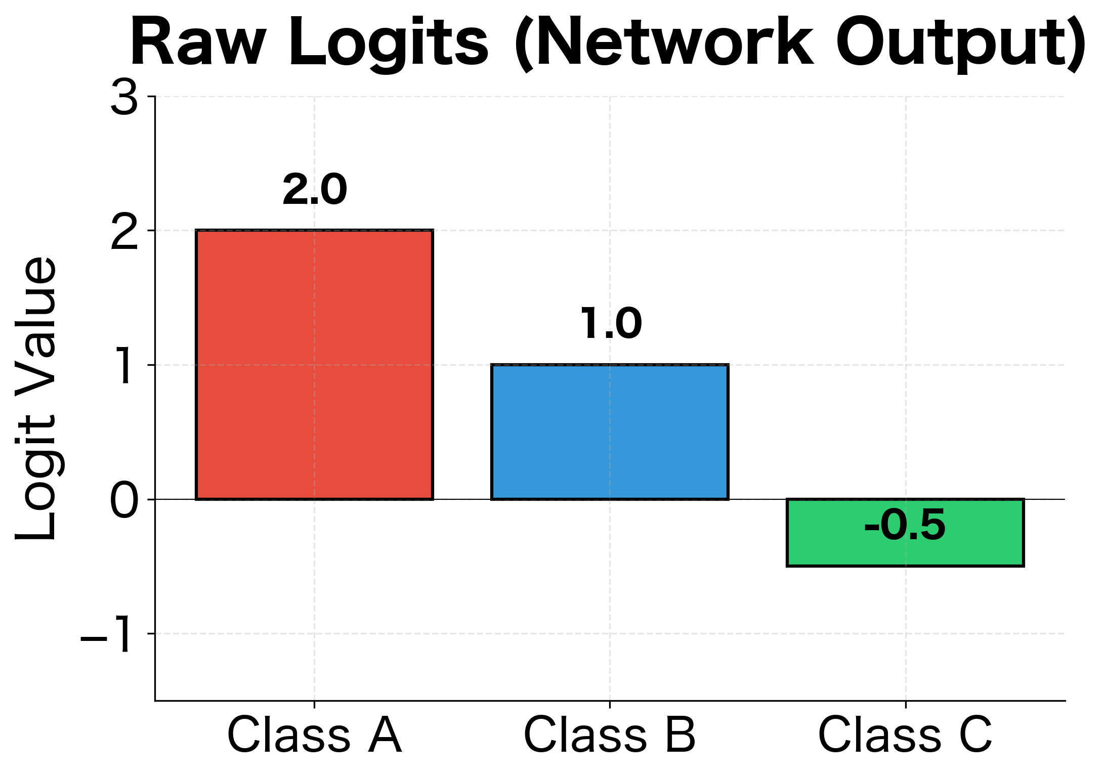
For problems with more than two classes, we use softmax activation in the output layer. Softmax converts a vector of raw scores (called logits) into a probability distribution. Given an output vector $\mathbf{z} = [z_1, z_2, \ldots, z_K]$ from the final layer, softmax computes the probability for each class:

where:

• $K$: the total number of classes
• $z_i$: the logit (raw score) for class $i$
• $e^{z_i}$: the exponential of $z_i$, which ensures all values become positive
• $\sum_{j=1}^{K} e^{z_j}$: the sum of exponentials across all classes, serving as a normalization constant

The exponential function amplifies differences between logits: if one class has a much higher score than others, it will dominate the probability distribution. The denominator ensures all probabilities sum to 1, creating a valid probability distribution where each output represents the predicted probability of the corresponding class.

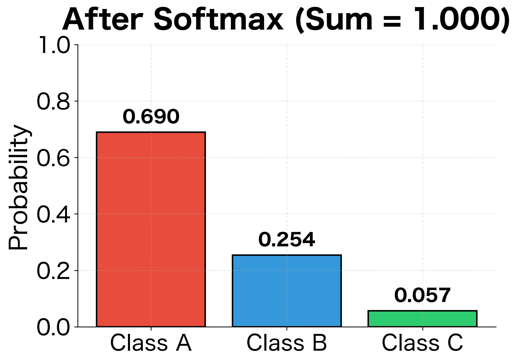
The multiclass model achieves high accuracy on the iris dataset, correctly classifying most test samples. Notice how the softmax outputs sum to 1.0 for each example, creating valid probability distributions. When the model is confident, one class dominates with probability close to 1.0 while others are near zero. The cross-entropy loss encourages this behavior by rewarding confident correct predictions and heavily penalizing confident incorrect ones.

Regression tasks require predicting continuous values rather than class labels. The key differences from classification are:

• No activation function on the output layer (identity function)
• Mean squared error (MSE) or mean absolute error (MAE) as the loss function
• Output layer has one neuron per target variable

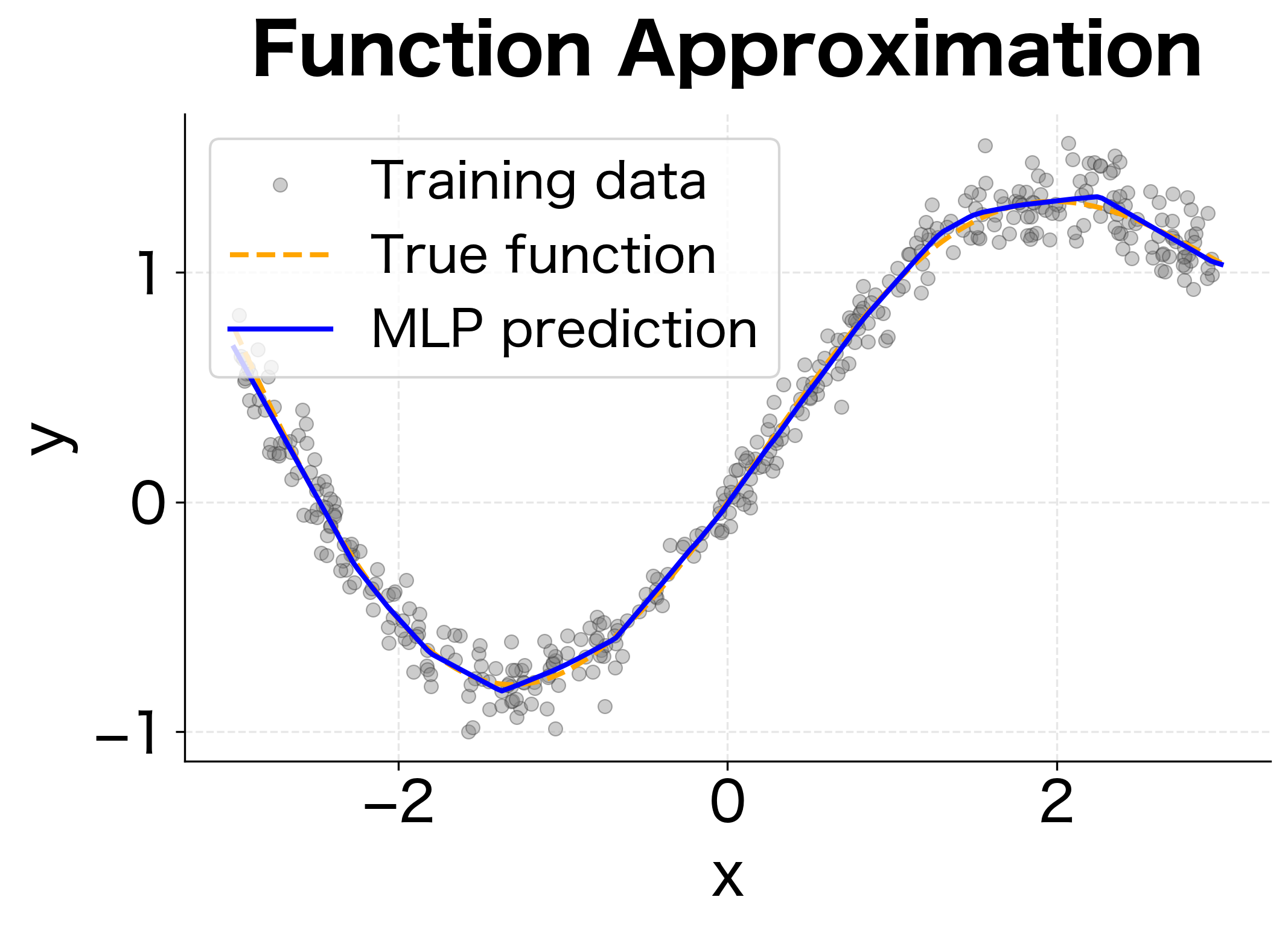
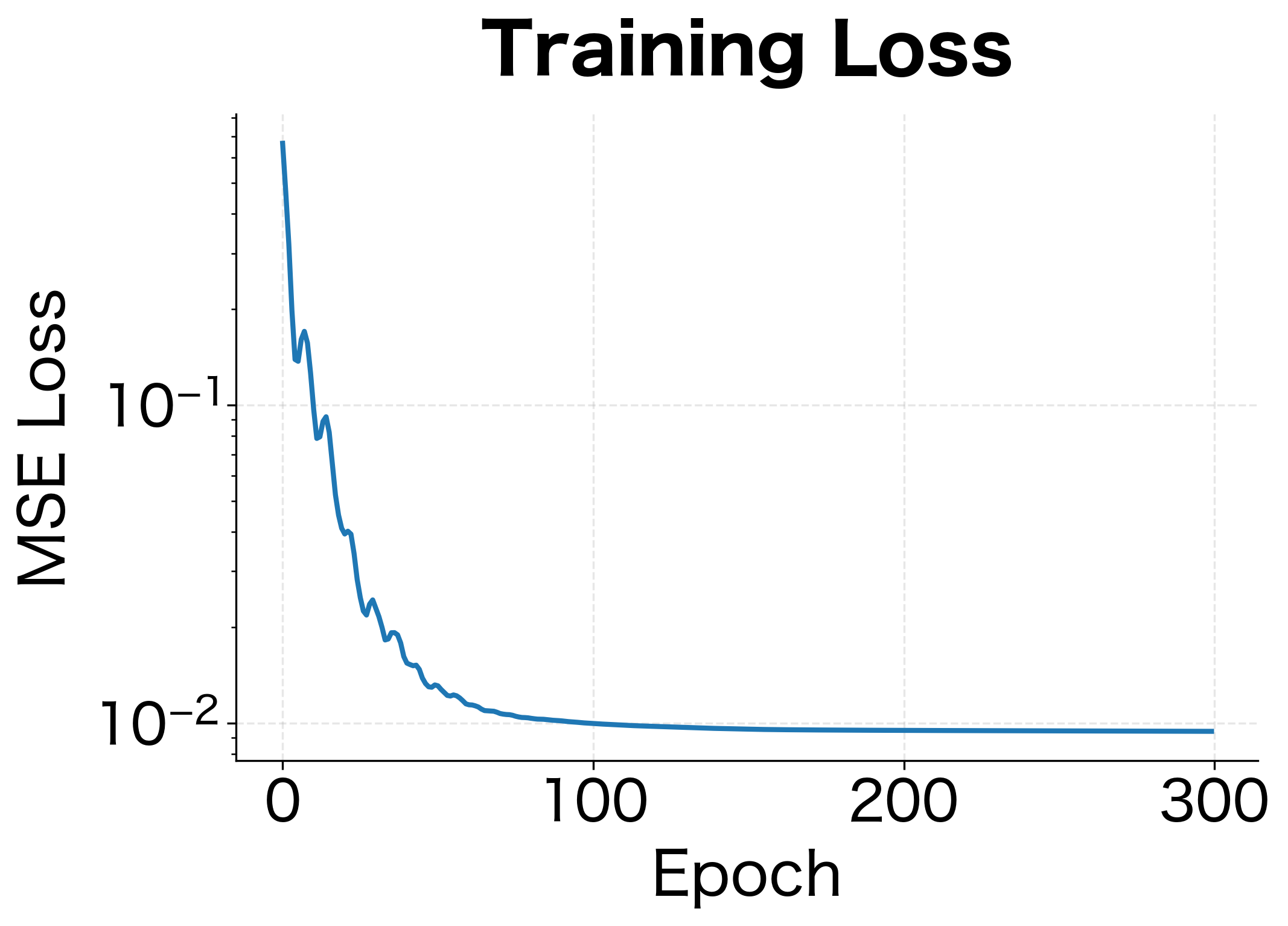
The low test MSE and RMSE indicate the model fits the underlying function well. The RMSE of around 0.1 means predictions are typically within 0.1 units of the true value on average, which matches the noise level we added to the data. The MLP learns to approximate the underlying non-linear function. Unlike polynomial regression where you must choose the degree, the MLP automatically discovers the appropriate level of complexity through its hidden representations.

Designing an MLP architecture involves choosing the number of layers, neurons per layer, activation functions, and regularization techniques. While there is no universal formula, several principles guide these decisions.

Deeper networks can represent more complex hierarchical features. However, they are harder to train due to vanishing or exploding gradients. Wider networks have more parameters per layer but may struggle to learn compositional patterns.

As a starting point:

• For simple problems, 1-2 hidden layers often suffice
• For complex patterns, 3-5 hidden layers may be needed
• Very deep networks (10+ layers) typically require residual connections

Common patterns for hidden layer sizes include:

• Funnel: Decreasing sizes (e.g., 256-128-64) that progressively compress information
• Constant: Same size throughout (e.g., 128-128-128) for uniform capacity
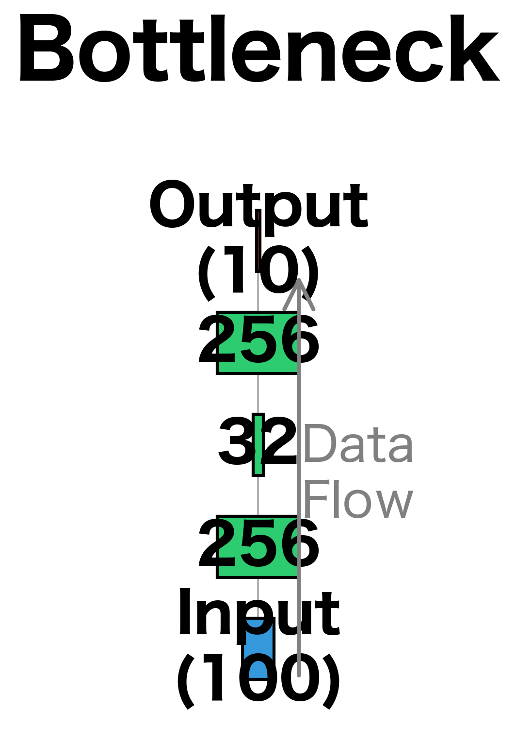
• Bottleneck: Narrow middle layer (e.g., 256-32-256) to force compressed representations

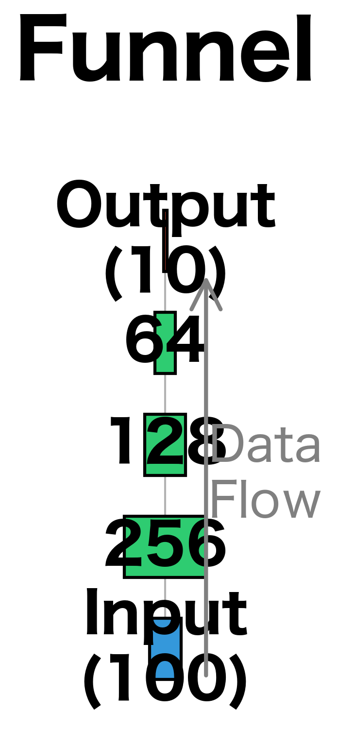
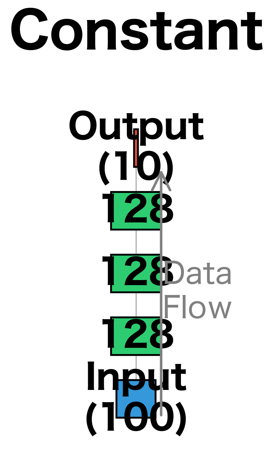
The input and output sizes are determined by your problem. Hidden sizes are hyperparameters to tune.

ReLU is the default choice for hidden layers due to its simplicity and effectiveness. Alternatives like Leaky ReLU or GELU can help in specific situations:

• ReLU: Fast, simple, works well in most cases
• Leaky ReLU/PReLU: Addresses dying ReLU problem
• GELU: Smooth approximation, popular in transformers
• Tanh/Sigmoid: Rarely used in hidden layers now due to saturation

For output layers:

• Sigmoid: Binary classification (outputs probability)
• Softmax: Multiclass classification (outputs probability distribution)
• Identity (none): Regression (outputs unbounded values)

To prevent overfitting, we use regularization techniques:

• Dropout: Randomly zeros neurons during training (typical rates: 0.2-0.5)
• Weight decay: L2 penalty on weights (typical values: 1e-4 to 1e-2)
• Batch normalization: Normalizes layer inputs, also acts as regularizer

This architecture applies batch normalization after each linear layer, followed by ReLU activation and dropout. The pattern Linear $\to$ BatchNorm $\to$ ReLU $\to$ Dropout repeats for each hidden layer, providing a consistent structure that's easy to extend. The funnel shape (256 $\to$ 128 $\to$ 64) progressively compresses the representation, forcing the network to distill the most important features as information flows toward the output.

Despite their power, MLPs have significant limitations that motivated the development of more specialized architectures.

The most fundamental limitation is their treatment of input as a flat vector. When processing images, MLPs ignore spatial structure, treating each pixel as an independent feature. A small shift in the image produces a completely different input vector, yet the semantic content remains the same. This lack of translation invariance means MLPs need to learn the same pattern multiple times for different positions. Convolutional neural networks address this by sharing weights across spatial locations.

Similarly, for sequential data like text, MLPs treat each position independently. The sentence "The cat sat on the mat" becomes a fixed-size vector where position 1 and position 5 have no structural relationship. This makes learning long-range dependencies extremely difficult. The meaning of "it" in "The trophy doesn't fit in the suitcase because it is too big" depends on understanding the full context, something MLPs struggle with. Recurrent networks and transformers were developed specifically to handle sequential dependencies.

MLPs also struggle with variable-length inputs. Every MLP has a fixed input size determined at architecture design time. Processing sentences of different lengths requires padding to a maximum length or using techniques like bag-of-words that lose positional information entirely. This rigidity limits their applicability to many real-world problems.

Despite these limitations, MLPs remain foundational. The feed-forward layers within transformers are MLPs. The classification heads on top of pre-trained language models are MLPs. Understanding how information flows through layers, how weights connect neurons, and how activations transform representations is essential knowledge for working with any modern neural architecture.

The representational power of MLPs demonstrated that neural networks could, in principle, learn complex functions. The universal approximation theorem provided theoretical justification. The practical challenge became not representation but optimization: finding the right weights among billions of possibilities. The techniques developed to train MLPs (gradient descent, backpropagation, and regularization) form the foundation of all deep learning.

Multilayer perceptrons extend single neurons into networks capable of learning complex, non-linear functions. By stacking layers with non-linear activations, MLPs can approximate virtually any function, a property formalized in the universal approximation theorem.

Key takeaways from this chapter:

• Hidden layers transform inputs into new representations where patterns become easier to detect
• Weight matrices connect layers, with shape $(n^{[l]}, n^{[l-1]})$ for the matrix connecting layer $l-1$ to layer $l$
• Forward pass propagates information through linear transformations and activations: $\mathbf{a}^{[l]} = \sigma(\mathbf{W}^{[l]} \mathbf{a}^{[l-1]} + \mathbf{b}^{[l]})$
• Batch processing uses matrix operations for efficiency, stacking examples as columns
• Classification uses sigmoid (binary) or softmax (multiclass) output activations with cross-entropy loss
• Regression uses identity (no) output activation with MSE loss
• Architecture design involves balancing depth, width, activation functions, and regularization

The next chapter explores loss functions in detail, examining how different choices affect learning and what happens when we optimize various objectives. Understanding loss functions is crucial because they define what "good" means for our network.

When building MLPs in PyTorch, several parameters significantly impact model performance:

Architecture Parameters:

• hidden_sizes: List of neurons per hidden layer (e.g., [256, 128, 64]). Larger sizes increase capacity but also parameter count and risk of overfitting. Start with powers of 2 for computational efficiency.
• input_size: Number of input features, determined by your data.
• num_classes / output_size: Number of output neurons. Use 1 for binary classification or regression, $K$ for $K$-class classification.

Regularization Parameters:

• dropout_rate: Probability of zeroing neurons during training (typically 0.1-0.5). Higher values provide stronger regularization but may slow convergence. Use 0.2-0.3 as a starting point.
• weight_decay: L2 regularization strength in the optimizer (typically 1e-4 to 1e-2). Penalizes large weights to reduce overfitting.

Training Parameters:

• lr (learning rate): Step size for gradient updates (typically 1e-4 to 1e-1). Too high causes instability; too low causes slow convergence. Adam optimizer often works well with lr=0.001.
• epochs: Number of complete passes through the training data. Monitor validation loss to avoid overfitting.
• batch_size: Number of examples per gradient update (typically 32-256). Larger batches provide more stable gradients but require more memory.

Activation Choices:

• Hidden layers: ReLU is the default choice. Consider Leaky ReLU if many neurons "die" (output constant zero).
• Output layer: Sigmoid for binary classification, Softmax (via CrossEntropyLoss) for multiclass, Identity (none) for regression.

Loss Functions:

• nn.BCELoss(): Binary cross-entropy for binary classification with sigmoid output.
• nn.CrossEntropyLoss(): Combines softmax and negative log-likelihood for multiclass classification. Expects raw logits, not probabilities.
• nn.MSELoss(): Mean squared error for regression tasks.

Ready to test your understanding of multilayer perceptrons? Take this quick quiz to reinforce what you've learned about hidden layers, forward pass computation, and network architecture.