

Learn how momentum transforms gradient descent by accumulating velocity to dampen oscillations and accelerate convergence. Covers intuition, math, Nesterov, and PyTorch implementation.

This article is part of the free-to-read Language AI Handbook
Choose your expertise level to adjust how many terms are explained. Beginners see more tooltips, experts see fewer to maintain reading flow. Hover over underlined terms for instant definitions.
Momentum
Gradient descent updates weights by stepping in the direction of steepest descent. But this greedy approach has a problem: it treats every step independently, ignoring the history of previous gradients. When the loss landscape is steep in some directions and shallow in others, vanilla gradient descent oscillates back and forth, making slow progress toward the minimum.
Momentum fixes this by adding memory to the optimization process. Instead of following only the current gradient, the optimizer accumulates a velocity that builds up over time. Like a ball rolling downhill, momentum carries the optimization past small bumps and narrow ravines, accelerating convergence in consistent directions while dampening oscillations in noisy ones.
This chapter develops momentum from intuition to implementation. You'll understand why the ball-rolling metaphor captures the core idea, derive the update equations, learn to choose the momentum coefficient, and see how momentum dramatically outperforms vanilla SGD on challenging loss surfaces.
The Ball Rolling Intuition
Imagine a ball rolling down a curved surface toward the lowest point. Two forces govern its motion: gravity pulls it downhill (the gradient), and its current velocity carries it forward even through flat regions or small upward slopes.
In physics, momentum is mass times velocity: , where is momentum, is mass, and is velocity. An object with momentum resists changes to its motion. The heavier and faster an object, the harder it is to stop or redirect.
This physical intuition maps directly to optimization. The gradient tells us the local direction of steepest descent, like gravity acting on the ball. But the ball doesn't instantly respond to every bump in the terrain. Its accumulated velocity smooths out the small-scale irregularities.
For neural network optimization, this smoothing effect is crucial. Loss surfaces are rarely simple bowls. They're riddled with narrow valleys, saddle points, and regions where the curvature differs wildly across dimensions. A ball with momentum can:
- Roll through flat regions without getting stuck
- Build up speed along consistent downhill directions
- Resist oscillations when the gradient keeps changing direction
- Escape shallow local minima by using built-up velocity
The key insight is that past gradients contain useful information. If the gradient has been pointing in the same direction for many steps, we should move faster in that direction. If it keeps alternating, we should slow down and average out the oscillations.
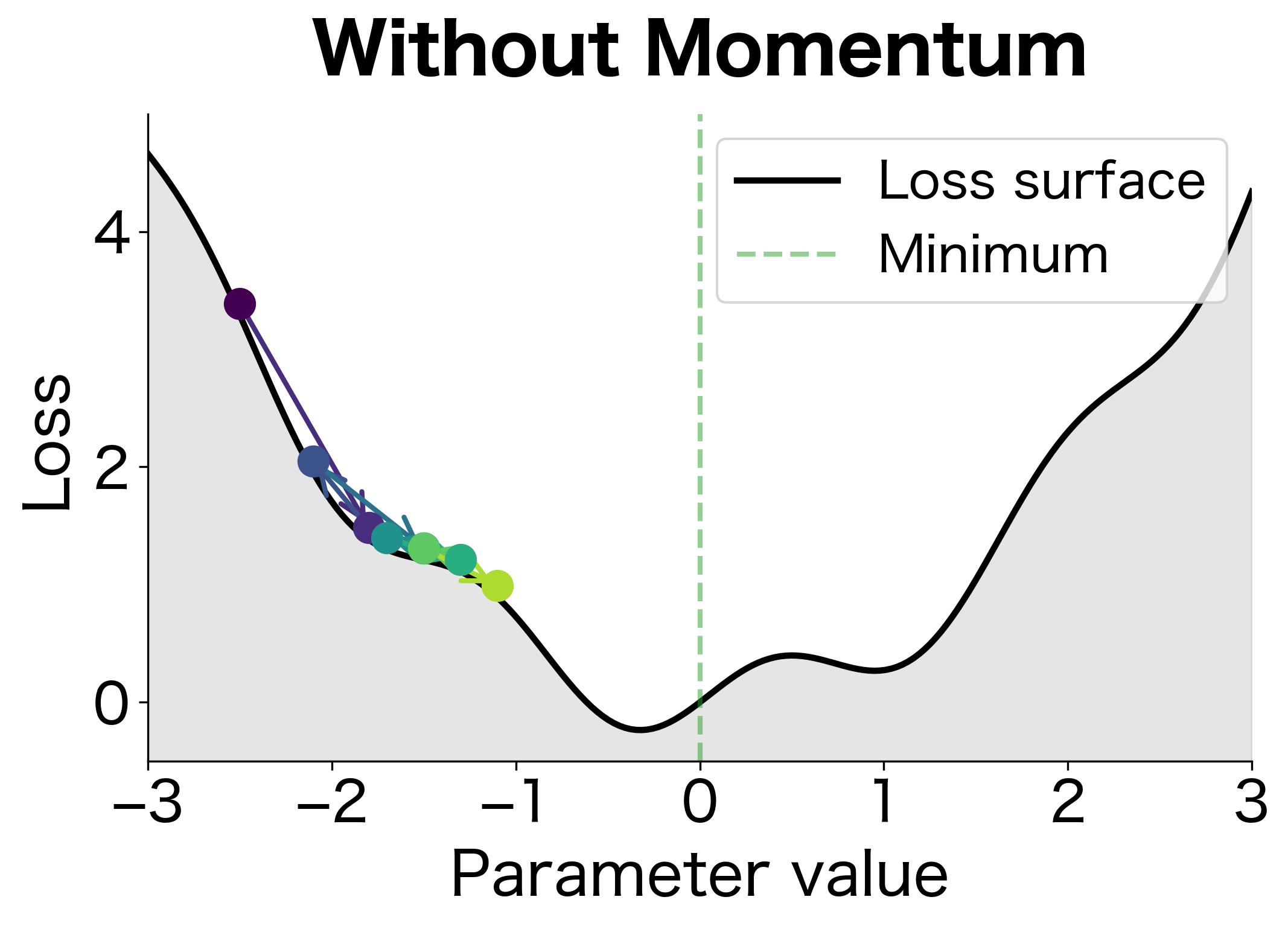
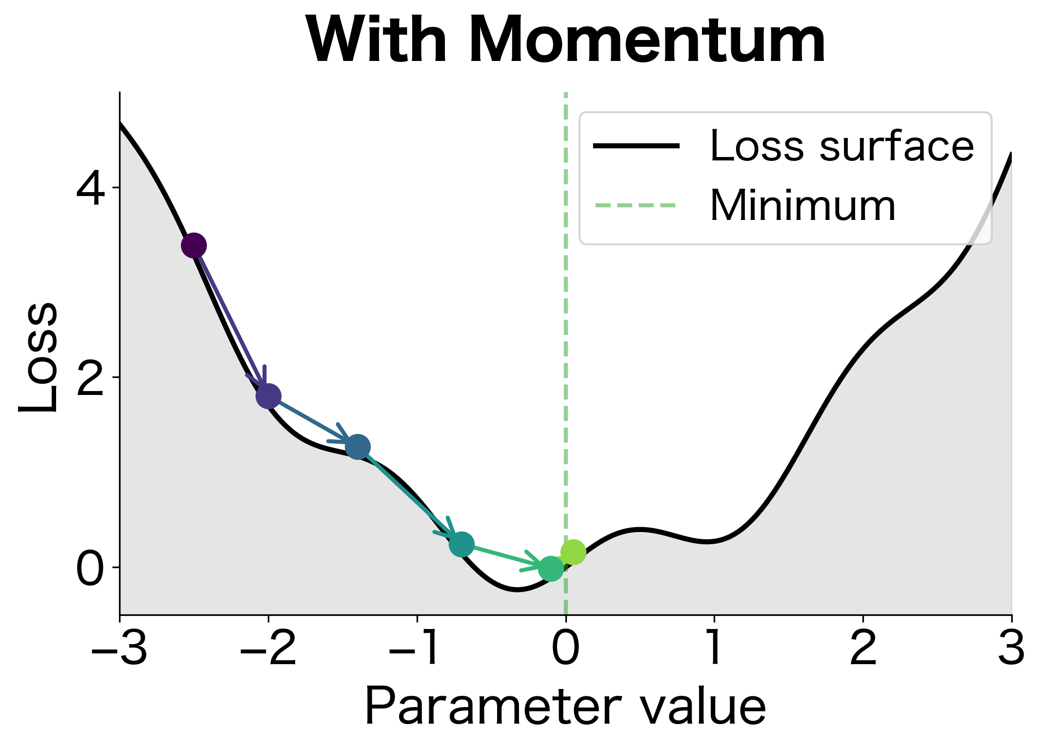
The first figure shows optimization without momentum. Each step follows only the current gradient, causing the ball to oscillate back and forth in the rippled valley. It makes progress but wastes energy reversing direction. The second figure shows momentum in action. The ball builds up velocity in the consistent downhill direction and smoothly rolls through the small bumps, reaching the minimum in fewer steps.
The Momentum Update Equations
To transform the ball-rolling intuition into a working algorithm, we need to formalize what "velocity" and "accumulation" mean mathematically. Let's build up the momentum update equations step by step, starting from vanilla gradient descent and showing exactly how momentum extends it.
Starting Point: Vanilla Gradient Descent
Standard gradient descent updates parameters by stepping in the direction opposite to the gradient:
where:
- : the parameter vector at time step (the current position on the loss surface)
- : the learning rate, controlling how large each step is
- : the gradient of the loss function at the current position (points uphill, so we subtract it to go downhill)
- : the updated parameters after taking one step
This update has a critical limitation: each step depends only on the current gradient. The optimizer has no memory of where it came from or how it got there. Every step is independent, as if the ball resets to zero velocity before each movement.
Introducing Velocity: The Key Insight
To give our optimizer memory, we introduce a velocity term that persists across time steps. Think of velocity as "where the optimizer wants to go based on everything it has seen so far." The update now splits into two parts:
Step 1: Update the velocity by blending the previous velocity with the new gradient:
Step 2: Update the parameters using the accumulated velocity:
Let's examine each component of the velocity update:
- : the velocity from the previous step, representing accumulated gradient history
- : the momentum coefficient (typically 0.9), determining how much of the old velocity to retain
- : the new gradient at the current position, adding fresh directional information
- : the updated velocity, a weighted combination of past and present
The parameter is the crucial control knob. It determines the balance between inertia (following the old direction) and responsiveness (following the new gradient).
The momentum coefficient determines how much of the previous velocity carries forward. A value of 0.9 means 90% of the old velocity is retained, blended with the new gradient. Higher values create more inertia (the ball is "heavier" and harder to redirect); lower values respond faster to new gradient information (the ball is "lighter" and more agile).
What Does Velocity Actually Compute?
The velocity equation (using for brevity) looks simple, but its recursive structure reveals something important. To understand what velocity really represents, let's unroll the recursion step by step.
Starting from rest: Assume the optimizer begins with zero velocity, . Now trace through the first few updates:
Step 1: The velocity is just the first gradient:
Step 2: The velocity blends the previous velocity (scaled by ) with the new gradient:
Step 3: Substituting and expanding:
The pattern emerges: At step , the velocity is a weighted sum of all past gradients, with exponentially decaying weights:
Each term in this sum tells us something important:
- : the most recent gradient, with weight 1 (full contribution)
- : the gradient from one step ago, with weight
- : the gradient from two steps ago, with weight
- And so on, with older gradients contributing exponentially less
This is an exponentially weighted moving average (EWMA) of gradients. Recent gradients dominate because they have smaller exponents, while distant gradients fade away. The result is a velocity that reflects the recent history of the loss landscape, not just a single point estimate.
Visualizing the Exponential Decay
How quickly do past gradients fade? With , let's compute the weights explicitly:
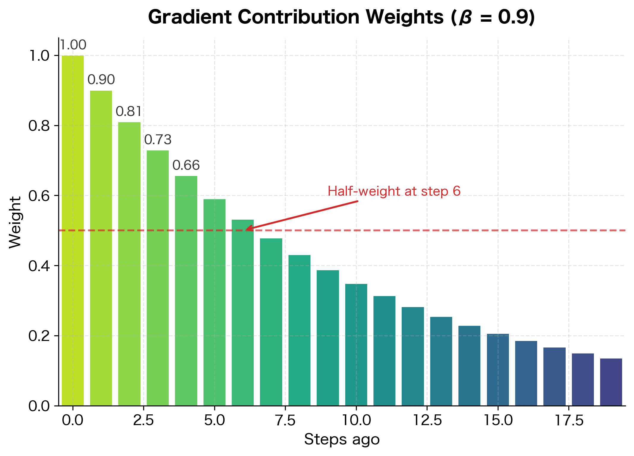
The most recent gradient contributes fully, but influence drops off quickly: after 10 steps, a gradient's weight has decayed to , and after 20 steps to just .
The Effective Window: How Many Gradients Matter?
The sum of all weights forms a geometric series. As we include more terms, the sum approaches a limit:
This formula tells us the effective window size of momentum. With :
Momentum effectively averages over approximately 10 recent gradients. This window size provides substantial smoothing while remaining responsive to gradient changes. Increasing to 0.99 expands the window to 100 gradients; decreasing to 0.5 shrinks it to just 2.
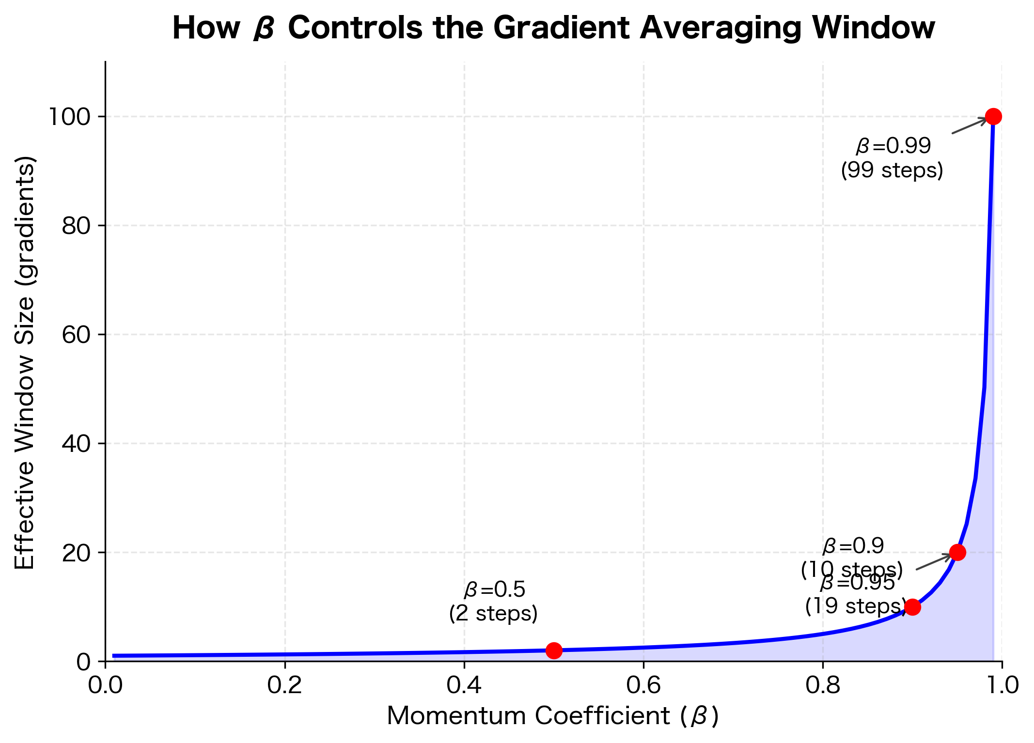
The hyperbolic relationship between and window size has practical implications: the difference between and is just 0.05, but it doubles the effective window from 10 to 20 gradients. Near , even tiny changes have dramatic effects.
Why Momentum Dampens Oscillations
Now we can explain precisely why momentum suppresses oscillations. The exponential averaging amplifies consistent signals while canceling out alternating ones.
The Mathematical Mechanism
Consider an optimizer navigating a narrow valley where the gradient alternates direction across the valley (steep walls) but points consistently along the valley floor. Let's trace through what happens.
Without momentum (equivalent to ), the optimizer responds to each gradient independently:
- Step 1: gradient is , move by
- Step 2: gradient is , move by
- Net displacement after 2 steps: zero
The optimizer bounces back and forth, making no progress.
With momentum (), the velocity accumulates history:
- Step 1: , move by
- Step 2: , move by
- Step 3: , move by
Notice what happens: the oscillating component shrinks from to to near-cancellation. After many steps, the alternating gradients average to nearly zero, and only the consistent component (if any) accumulates in the velocity.
Two Contrasting Cases
To see this cancellation effect clearly, compare two scenarios:
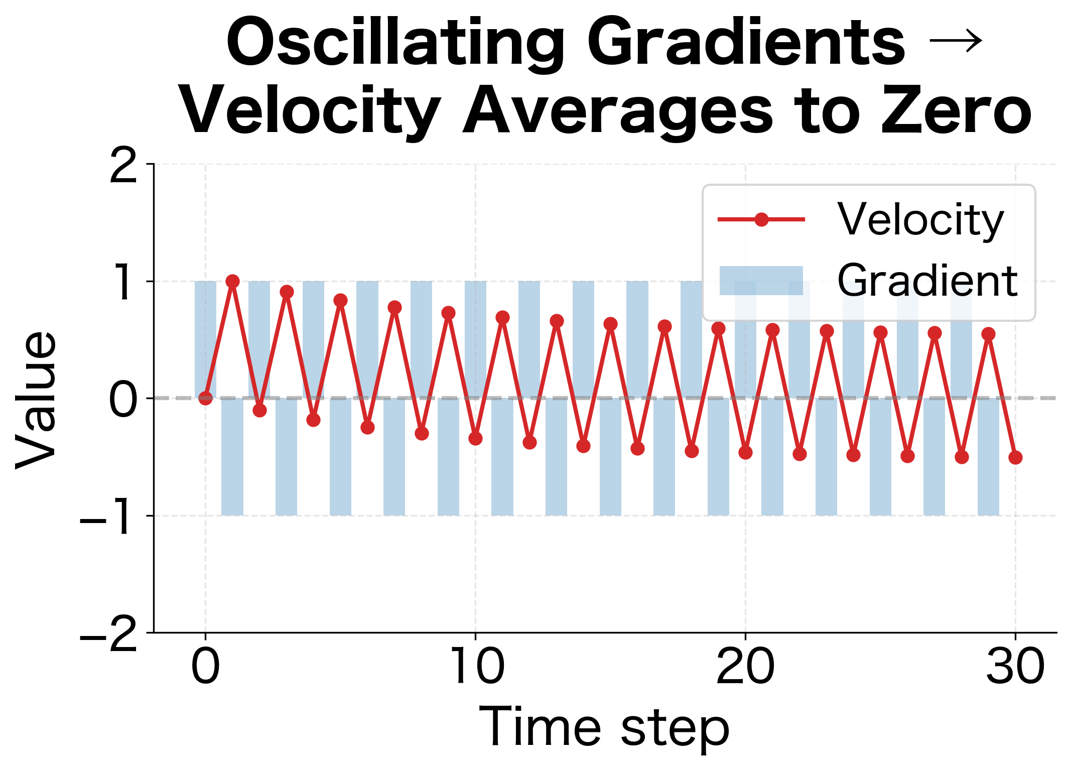
- Oscillating gradients: If gradients alternate , the velocity quickly stabilizes near zero
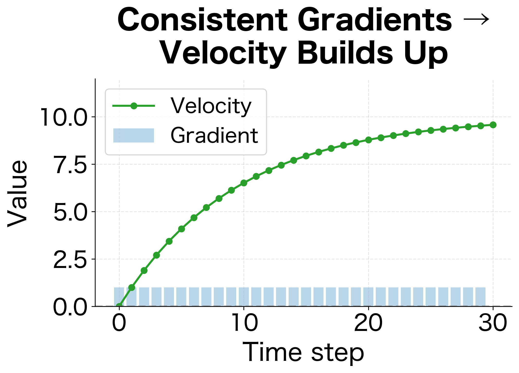
- Consistent gradients: If gradients are always , the velocity builds up toward
Let's simulate both cases to see the velocity evolution:
The visualization reveals the stark contrast:
-
Oscillating gradients (first figure): Despite gradients alternating between +1 and -1 with full magnitude, the velocity (red line) quickly settles near zero. The exponential averaging causes opposing gradients to cancel, preventing wasted motion across the valley.
-
Consistent gradients (second figure): With gradients always pointing the same direction, velocity (green line) grows steadily toward the theoretical limit of . The optimizer accelerates along the consistent direction, taking steps up to 10x larger than vanilla SGD.
The Signal-Noise Interpretation
This asymmetric behavior reveals momentum's core capability: it acts as a filter that separates signal from noise in the gradient stream.
- Signal: Gradient components that consistently point in the same direction represent the true direction toward the minimum. Momentum amplifies these.
- Noise: Gradient components that oscillate back and forth represent either stochasticity (mini-batch variance) or curvature mismatch (narrow valleys). Momentum suppresses these.
This automatic filtering is why momentum works so well in practice. The optimizer doesn't need to know which directions are "signal" and which are "noise." The mathematical structure of exponential averaging naturally makes that distinction.
Choosing the Momentum Coefficient
The momentum coefficient controls the trade-off between stability and responsiveness:
- Higher (0.95-0.99): More smoothing, stronger acceleration in consistent directions, but slower adaptation to changing gradients
- Lower (0.8-0.9): Faster response to new gradient information, but less accumulation and dampening
- : Equivalent to vanilla SGD (no momentum)
The standard choice is , which works well across most problems. This value provides substantial smoothing (averaging roughly 10 recent gradients) while still adapting reasonably quickly to loss landscape changes.
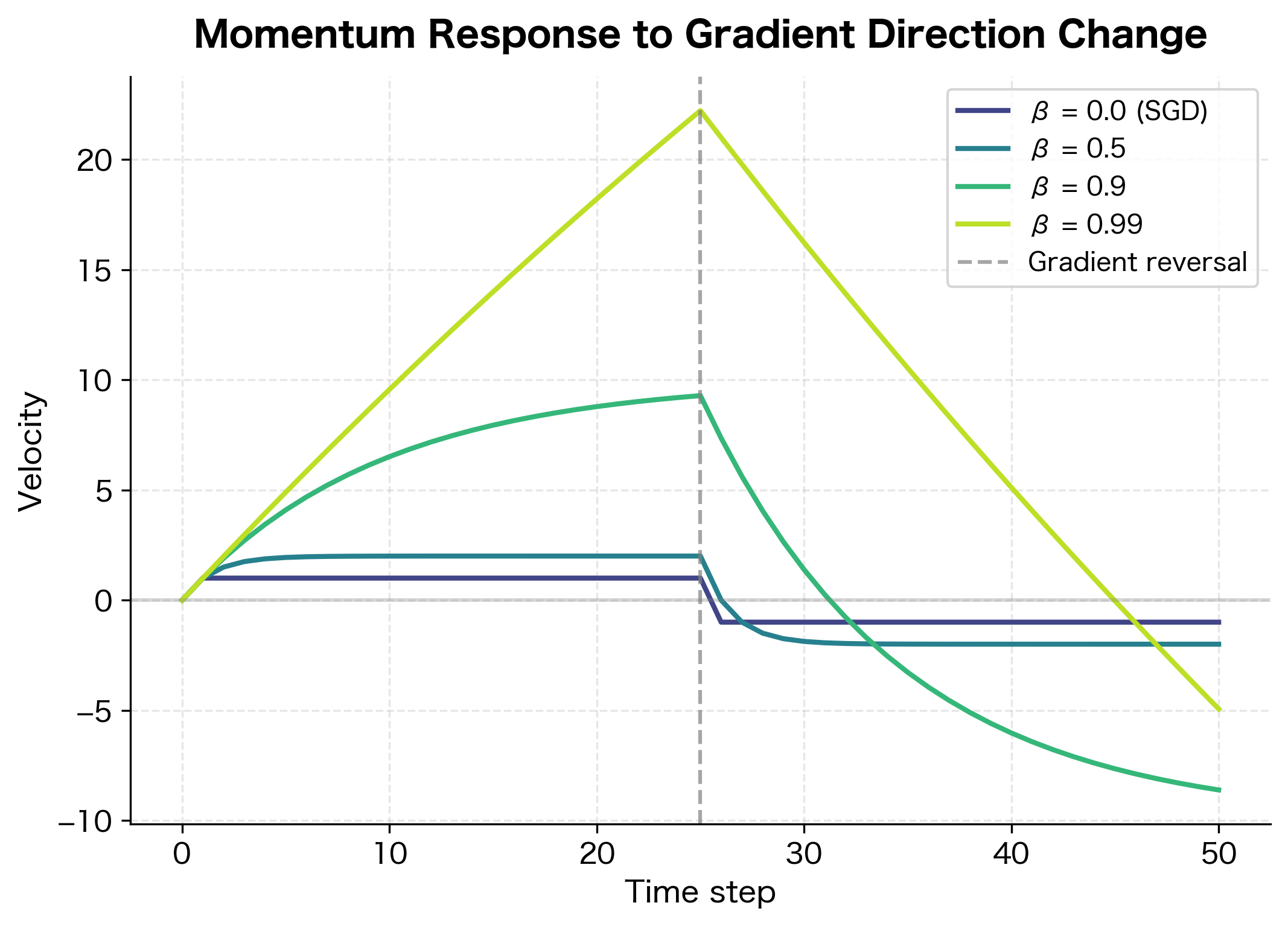
The plot reveals the trade-off clearly. With (vanilla SGD), velocity instantly tracks the gradient. With , velocity builds to nearly 100 but takes many steps to reverse after the gradient flips. The standard offers a balance: substantial acceleration during consistent phases, yet reasonable response time when the landscape changes.
For problems with noisy gradients (small batch sizes), higher momentum helps smooth out the noise. For problems requiring rapid adaptation (non-stationary objectives), lower momentum is preferred.
Momentum vs Vanilla SGD
Let's compare momentum and vanilla SGD on a challenging optimization problem: a narrow valley where the gradient is steep across the valley (causing oscillations) but shallow along the valley floor (requiring many steps to reach the minimum).
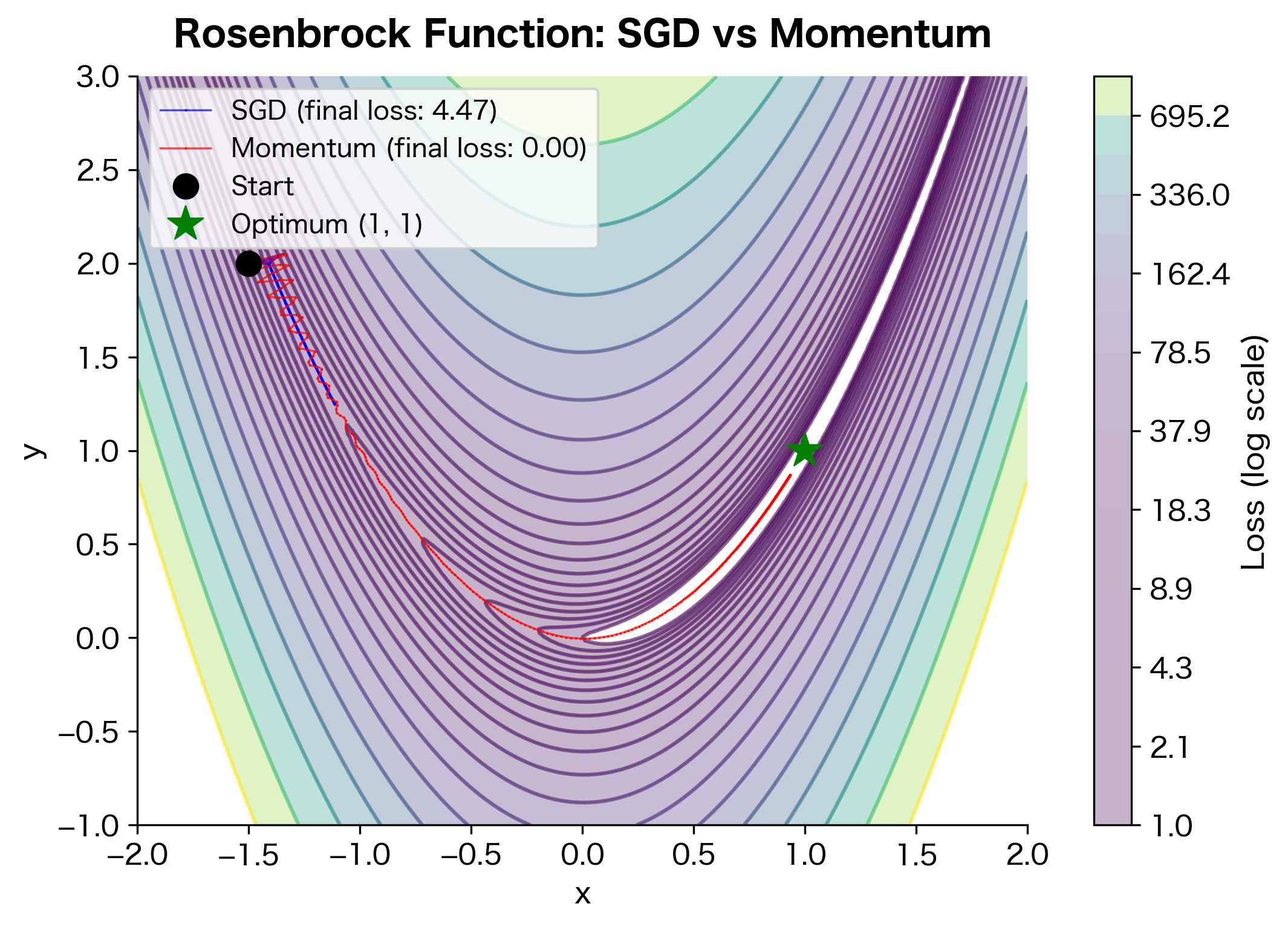
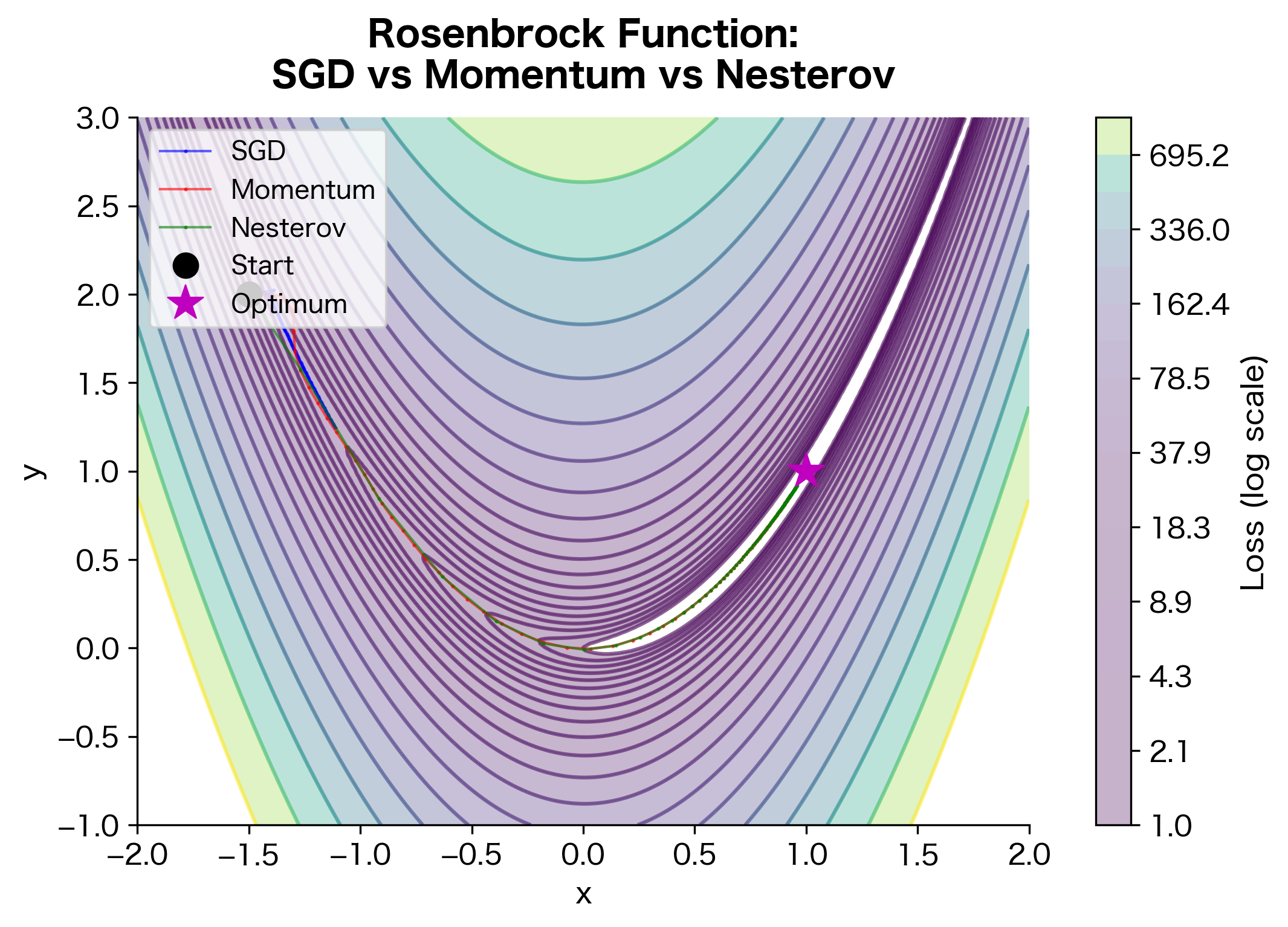
The Rosenbrock function has a narrow curved valley leading to the minimum at (1, 1). Vanilla SGD struggles because the steep valley walls create large gradients that push the optimizer back and forth across the valley. Meanwhile, the shallow gradient along the valley floor means slow progress toward the minimum.
Momentum solves both problems. The oscillating component of the gradient (across the valley) averages out, while the consistent component (along the valley) accumulates. The result: smoother, faster convergence.
The improvement factor quantifies momentum's advantage on this problem. A factor greater than 1 means momentum reached a lower loss than vanilla SGD in the same number of steps. On the Rosenbrock function, momentum's ability to dampen cross-valley oscillations while accelerating along-valley progress results in substantially faster convergence.
Nesterov Momentum
Standard momentum computes the gradient at the current position before taking a step. But since we know we're about to move in the direction of the current velocity, why not compute the gradient at the anticipated future position instead? This is the key insight behind Nesterov accelerated gradient (NAG).
Nesterov momentum, also called Nesterov accelerated gradient (NAG), computes the gradient at the "look-ahead" position rather than the current position. This provides a form of correction: if the velocity is pointing in the wrong direction, the gradient at the look-ahead position helps correct course before committing to the full step.
The Nesterov update equations modify the velocity update to use a "look-ahead" gradient:
where:
- : the velocity at time step
- : the momentum coefficient (same as standard momentum)
- : the "look-ahead" position, approximating where the velocity would carry us
- : the gradient evaluated at the look-ahead position rather than the current position
- : the learning rate
The key difference from standard momentum is in the first equation: instead of computing at the current position, we compute at the anticipated future position. This allows the optimizer to "peek ahead" and adjust course before committing to the full step.
Why Look Ahead?
Consider what happens when the optimizer is approaching a minimum at high velocity. Standard momentum computes the gradient at the current position and adds it to the velocity, potentially overshooting. Nesterov momentum looks ahead to see where the velocity is taking us, then computes the gradient there.
If we're about to overshoot, the look-ahead gradient points back toward the minimum, helping brake before it's too late. If we're on track, the look-ahead gradient reinforces the current direction.
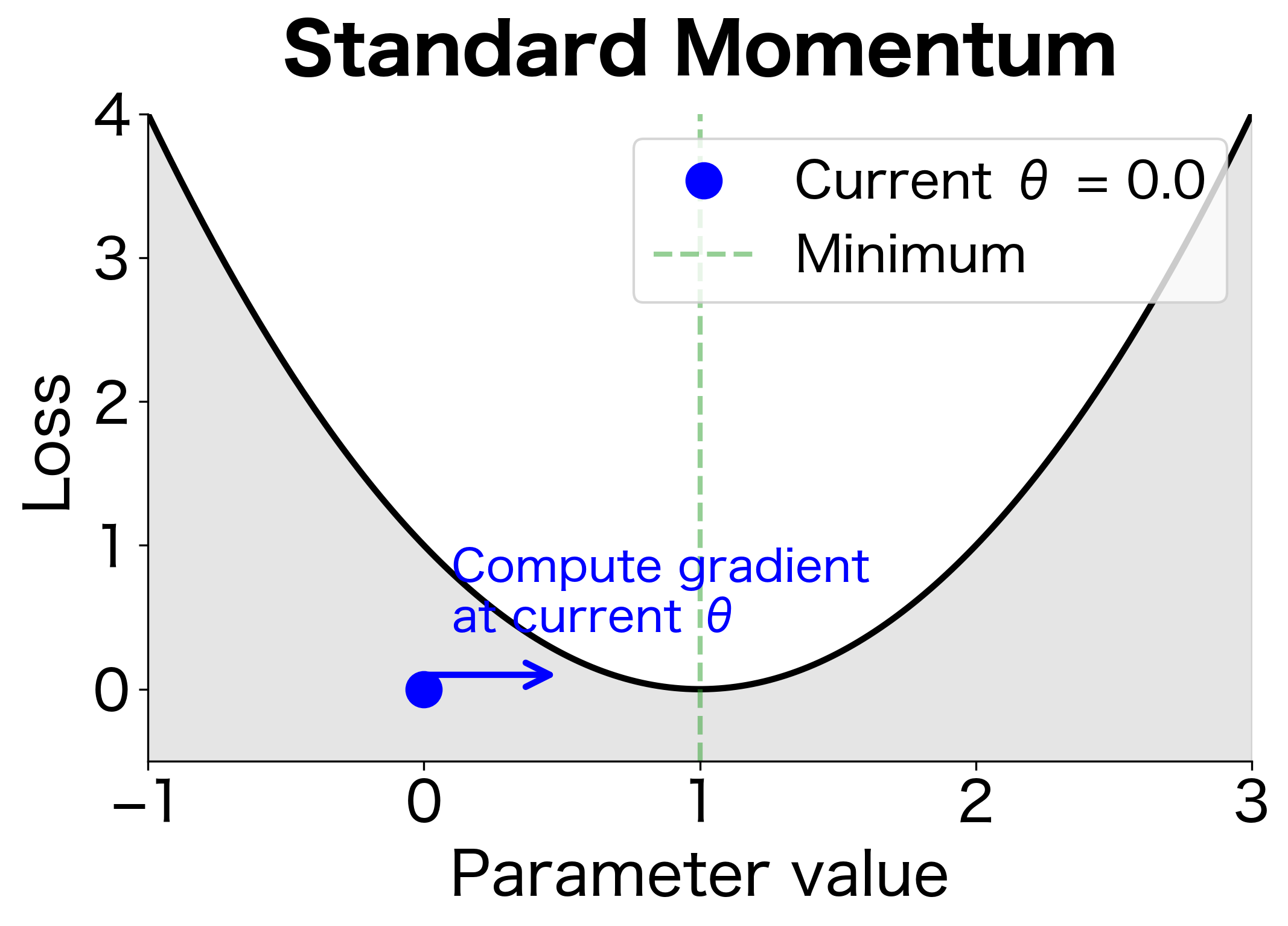
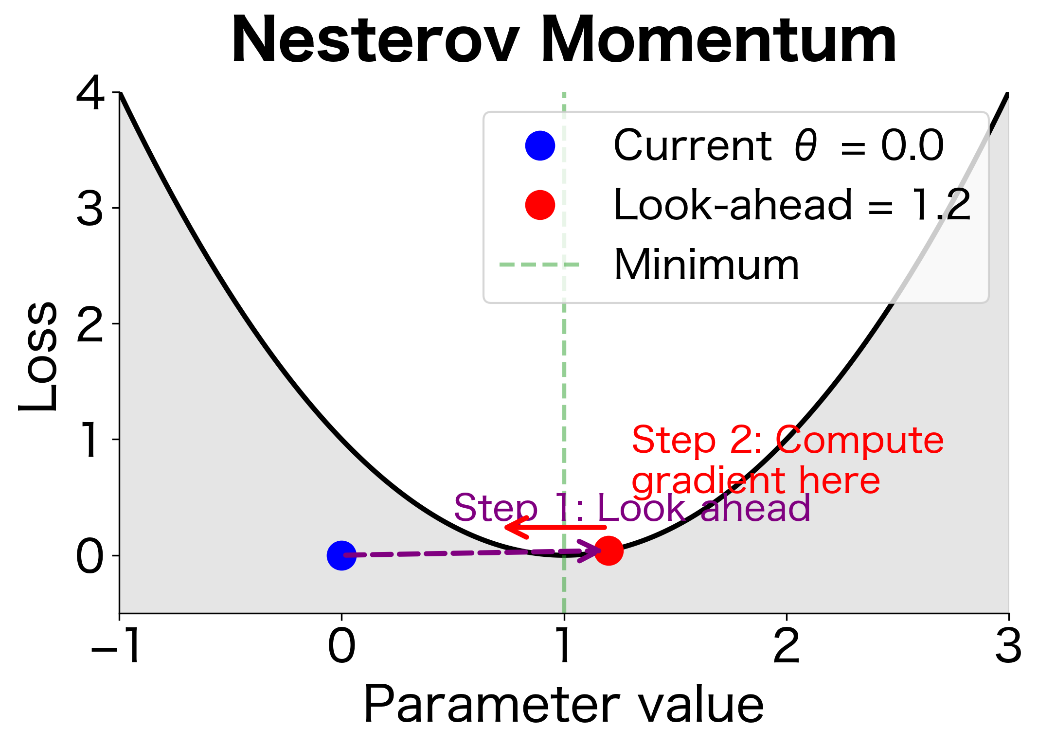
The diagram shows why Nesterov helps near minima. With standard momentum, we compute the gradient at , which still points toward the minimum. But the velocity is carrying us past it. With Nesterov, we look ahead to , where the gradient points back, signaling that we're about to overshoot. This allows earlier correction.
Implementing Nesterov Momentum
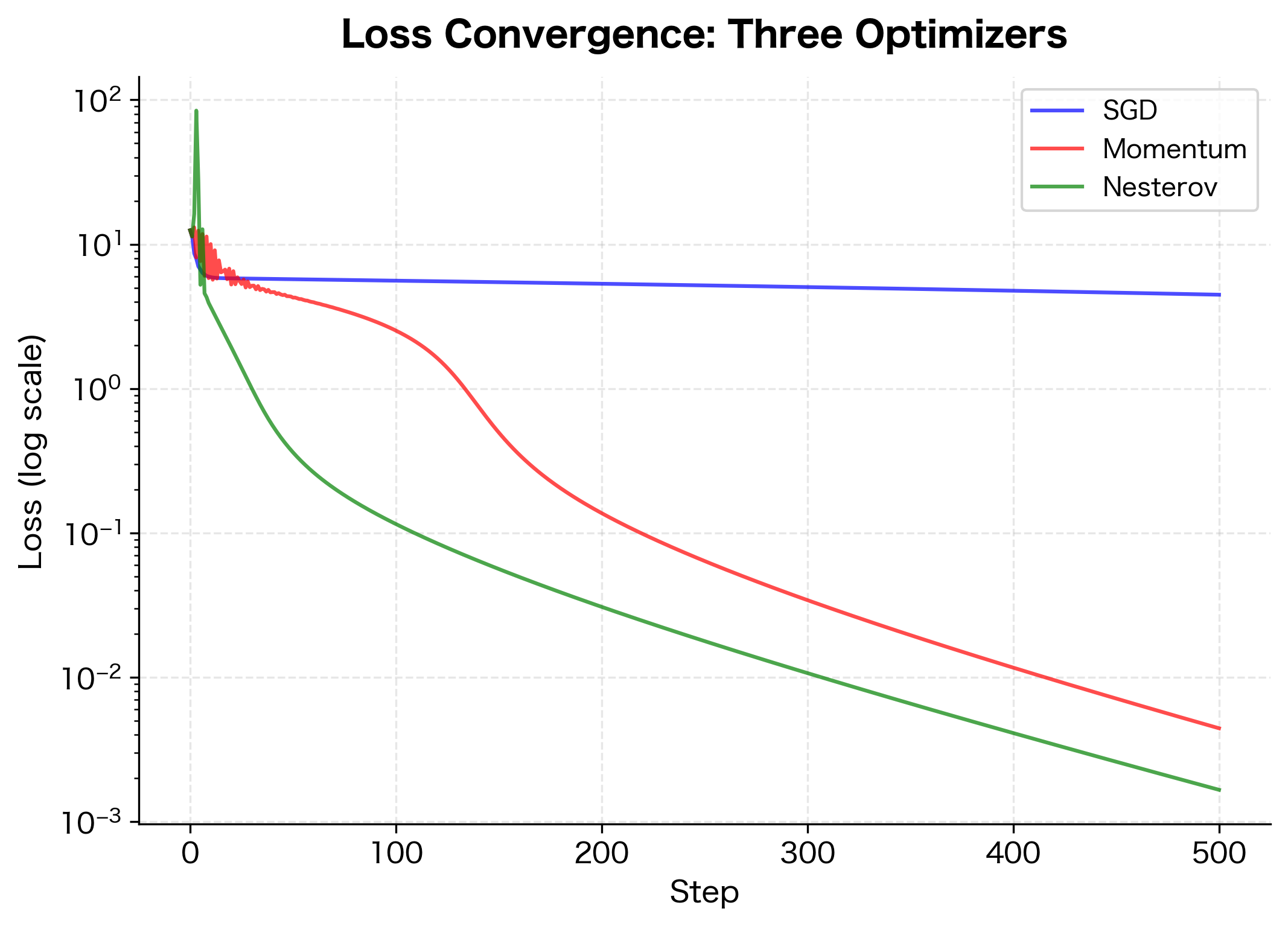
The final loss values show the ranking: Nesterov reaches the lowest loss, followed by standard momentum, with vanilla SGD trailing behind. The gap between momentum and Nesterov is typically smaller than the gap between SGD and momentum, reflecting that the look-ahead correction provides incremental rather than transformative improvement.
Nesterov momentum typically converges faster than standard momentum, especially on convex problems. The theoretical convergence rate for Nesterov on smooth convex functions is , compared to for vanilla gradient descent.
Here, means the optimization error decreases proportionally to after iterations. In practical terms:
- Vanilla gradient descent: After 100 steps, error is roughly proportional to
- Nesterov momentum: After 100 steps, error is roughly proportional to
This quadratic improvement is significant: Nesterov reaches the same accuracy in roughly steps compared to vanilla gradient descent. In practice, Nesterov often provides a modest but consistent improvement over standard momentum.
Implementing Momentum in PyTorch
PyTorch's SGD optimizer includes momentum as a built-in option. Let's see how to use it and verify our understanding:
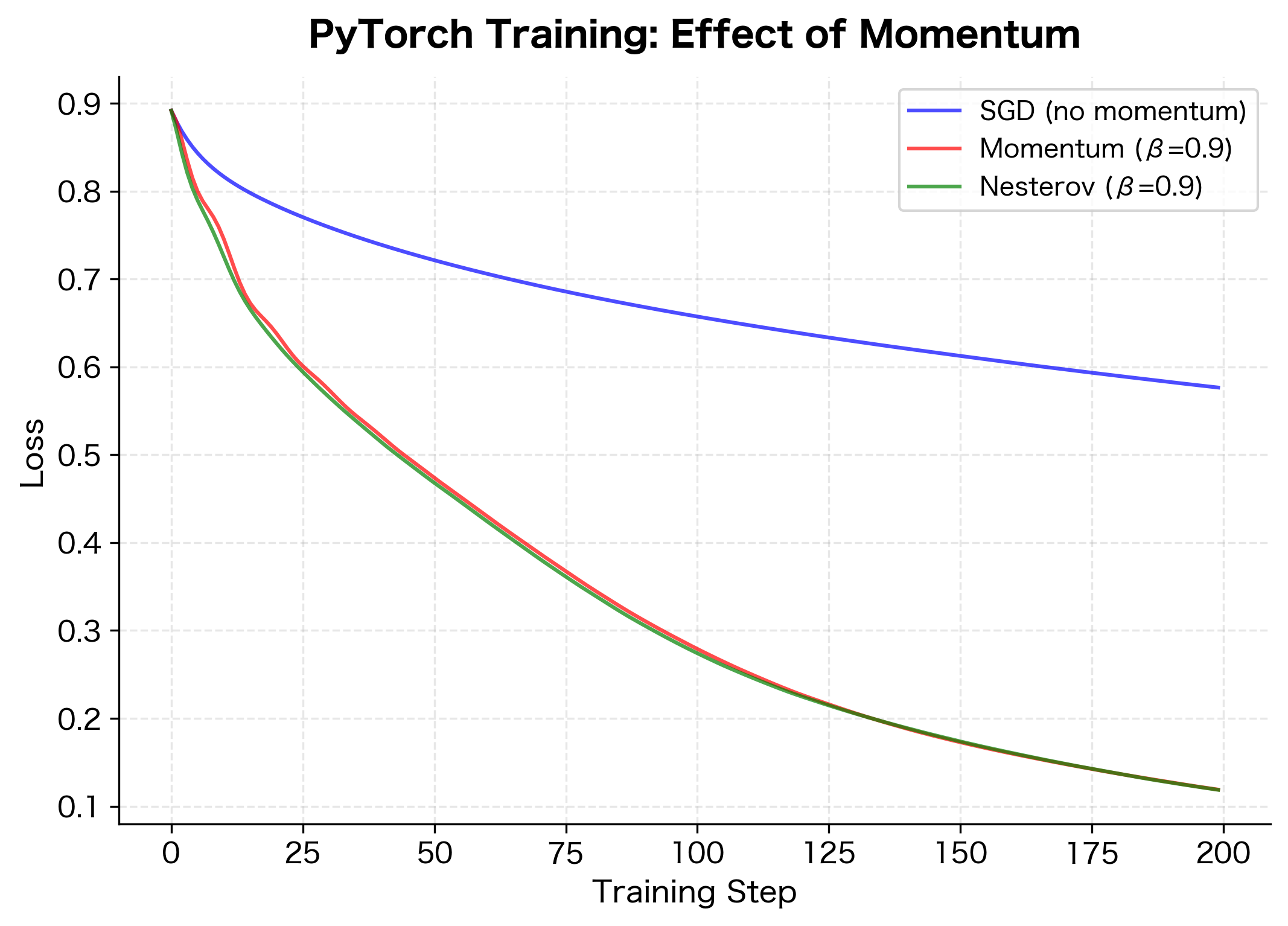
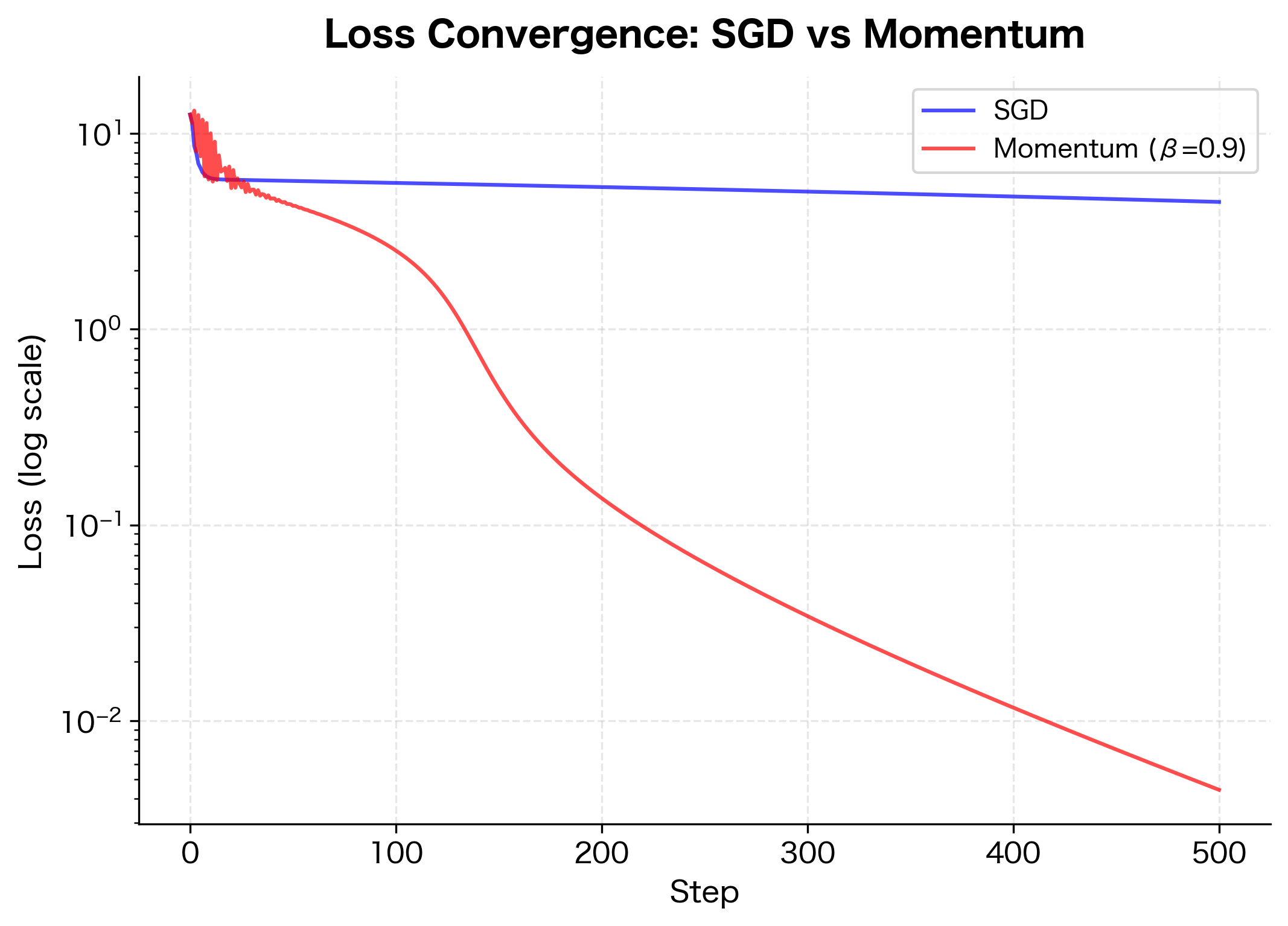
The training curves demonstrate momentum's practical benefit. With no momentum, training shows more oscillation and slower convergence. Both standard and Nesterov momentum smooth out the training and reach lower loss values faster.
Implementing Momentum from Scratch
To solidify understanding, let's implement momentum manually and verify it matches PyTorch's behavior:
A small difference between the implementations is expected due to floating-point precision, but the values should be nearly identical. If the max difference is on the order of or smaller, our manual implementation correctly replicates PyTorch's momentum algorithm. Larger discrepancies would indicate a bug in the implementation logic.
Momentum Hyperparameter Guidelines
Choosing appropriate momentum settings depends on your problem and other hyperparameters:
Momentum Coefficient ()
- 0.9: The default choice for most problems. Provides good balance between acceleration and responsiveness.
- 0.95-0.99: Use for very noisy gradients (small batch sizes) or when you want stronger smoothing.
- 0.8-0.85: Use when the loss landscape changes rapidly or you need faster adaptation.
Interaction with Learning Rate
Momentum effectively amplifies the learning rate. When the gradient points consistently in the same direction, velocity accumulates toward a steady-state value. For a constant gradient , the velocity converges to:
where:
- : the steady-state velocity after many steps of consistent gradient
- : the constant gradient value
- : the momentum coefficient
- : the "leak" factor that prevents velocity from growing unboundedly
With , the effective step size becomes , which is 10x larger than vanilla SGD's step of . You may need to reduce the learning rate when adding momentum to prevent overshooting.
| Momentum β | Amplification Factor |
|---|---|
| 0.0 | 1.0× |
| 0.5 | 2.0× |
| 0.9 | 10.0× |
| 0.99 | 100.0× |
As approaches 1, the amplification factor grows without bound. With , the effective step size is 100x larger than vanilla SGD. This is why practitioners often reduce the learning rate when switching from vanilla SGD to momentum, or when increasing the momentum coefficient.
When adding momentum to vanilla SGD, consider reducing the learning rate by a factor of to maintain similar step sizes.
Batch Size Interaction
Larger batch sizes produce more stable gradient estimates, reducing the need for momentum's smoothing effect. With very large batches, you might reduce momentum slightly. With small batches, higher momentum helps average out the noise.
Limitations and When Not to Use Momentum
Momentum isn't always beneficial:
- Highly non-convex landscapes: Momentum can carry the optimizer past good local minima into worse regions.
- Rapidly changing objectives: In reinforcement learning or meta-learning, the optimal direction changes frequently, and momentum's memory becomes a liability.
- Very noisy gradients: While momentum helps with moderate noise, extremely noisy gradients can corrupt the velocity estimate.
Modern optimizers like Adam combine momentum with adaptive learning rates, often outperforming pure momentum SGD. However, momentum remains a fundamental technique, and understanding it is essential for grasping how Adam and similar optimizers work.
Momentum's impact on deep learning has been substantial. Before momentum became standard practice, training deep networks was notoriously difficult. The dampening of oscillations and acceleration of convergence made previously intractable problems solvable. Today, momentum is baked into nearly every optimizer used in practice, from SGD with momentum to Adam's first moment estimate.
Key Parameters
When configuring momentum-based optimizers, the following parameters have the greatest impact on training dynamics:
-
momentum(β): The momentum coefficient controls how much of the previous velocity carries forward to the next step. Range: 0.0 to 0.99 (values ≥ 1.0 cause divergence). Default: 0.9. Higher values provide more smoothing and acceleration but slower adaptation to gradient changes. Start with 0.9, increase to 0.95-0.99 for noisy gradients (small batches), or decrease to 0.8-0.85 if the loss landscape changes rapidly. -
lr(learning rate): The step size for parameter updates. With momentum, the effective step size is amplified by up to . When adding momentum to vanilla SGD, consider reducing the learning rate by a factor of to maintain similar step magnitudes. Example: if vanilla SGD useslr=0.1and you addmomentum=0.9, trylr=0.01as a starting point. -
nesterov: Boolean flag to enable Nesterov accelerated gradient instead of standard momentum. Default:Falsein PyTorch. Computes gradients at a look-ahead position, providing earlier feedback about overshooting. Generally safe to enable; provides modest but consistent improvement, especially on convex problems. -
dampening(PyTorch-specific): Reduces the contribution of the current gradient to the velocity update. Default: 0 (no dampening). Withdampening=d, the update becomes . Rarely modified; leave at 0 unless you have specific reasons to dampen gradient contributions.
Summary
Momentum enhances gradient descent by accumulating a velocity that smooths optimization trajectories and accelerates convergence in consistent directions.
Key takeaways:
- Velocity accumulation creates an exponentially weighted average of past gradients
- Dampening effect cancels out oscillating gradient components
- Acceleration amplifies consistent gradient directions by up to (e.g., 10x when )
- Momentum coefficient is the standard choice, balancing smoothing and responsiveness
- Nesterov momentum looks ahead before computing gradients, providing earlier feedback about overshooting
- Learning rate interaction means you may need to reduce learning rate when adding momentum
- PyTorch integration is straightforward via
torch.optim.SGD(momentum=0.9, nesterov=True)
Momentum transforms the greedy, memoryless nature of vanilla gradient descent into a more intelligent optimization process that learns from the history of gradients. This simple idea, inspired by physical intuition, remains one of the most important techniques in neural network optimization.
Quiz
Ready to test your understanding? Take this quick quiz to reinforce what you've learned about momentum in neural network optimization.

Comments