Search

Search articles

Part-of-Speech Tagging: Tag Sets, Algorithms & Implementation

Michael BrenndoerferDecember 15, 202535 min read

Learn POS tagging from tag sets to statistical taggers. Covers Penn Treebank, Universal Dependencies, emission and transition probabilities, and practical implementation with NLTK and spaCy.

Reading Level

Choose your expertise level to adjust how many terms are explained. Beginners see more tooltips, experts see fewer to maintain reading flow. Hover over underlined terms for instant definitions.

Part-of-Speech Tagging

Every word in a sentence plays a role. Nouns name things, verbs describe actions, adjectives modify nouns, and adverbs modify verbs. Part-of-speech tagging is the task of automatically labeling each word with its grammatical category. Given the sentence "The quick brown fox jumps over the lazy dog," a POS tagger produces labels like DET, ADJ, ADJ, NOUN, VERB, ADP, DET, ADJ, NOUN.

Why does this matter? Part-of-speech information forms the backbone of deeper linguistic analysis. Syntactic parsers use POS tags to constrain the possible parse trees. Named entity recognizers rely on POS patterns to identify entity boundaries. Information extraction systems use verb-noun sequences to find relations. Even modern neural systems, despite learning representations end-to-end, often benefit from POS features as auxiliary inputs.

This chapter introduces the fundamental concepts of POS tagging. You'll learn the major tag sets used in NLP, understand why context matters for disambiguation, implement taggers using both rules and statistical methods, and evaluate their performance on real text.

What Is a Part of Speech?

Parts of speech, also called lexical categories or word classes, group words by their grammatical function and syntactic behavior. Linguists have debated these categories for millennia, dating back to Pāṇini's grammar of Sanskrit around 500 BCE.

Part of Speech

A part of speech (POS) is a category of words that share similar grammatical properties and syntactic roles. Examples include nouns, verbs, adjectives, adverbs, prepositions, and conjunctions.

Traditional grammar identifies eight parts of speech in English: noun, verb, adjective, adverb, pronoun, preposition, conjunction, and interjection. Computational linguistics uses finer distinctions. Instead of just "verb," we might distinguish between base verbs (VB), third-person singular present verbs (VBZ), past tense verbs (VBD), and past participles (VBN).

Consider how the word "run" behaves differently in these sentences:

  • "I run every morning." (base verb, VB)
  • "She runs every morning." (third-person singular, VBZ)
  • "He ran yesterday." (past tense, VBD)
  • "I have run marathons before." (past participle, VBN)
  • "That was a good run." (noun, NN)

The same word form can have different tags depending on context. This ambiguity is what makes POS tagging challenging and interesting.

Tag Sets

A tag set defines the inventory of labels a tagger can assign. Different tag sets make different distinctions, trading off between granularity and simplicity.

The Penn Treebank Tag Set

The Penn Treebank tag set, developed at the University of Pennsylvania in the 1990s, became the de facto standard for English POS tagging. It contains 36 POS tags plus 12 punctuation and symbol tags.

In[2]:
Code
# Penn Treebank tag set (core POS tags)
penn_tags = {
    # Nouns
    "NN": "Noun, singular or mass",
    "NNS": "Noun, plural",
    "NNP": "Proper noun, singular",
    "NNPS": "Proper noun, plural",
    # Verbs
    "VB": "Verb, base form",
    "VBD": "Verb, past tense",
    "VBG": "Verb, gerund or present participle",
    "VBN": "Verb, past participle",
    "VBP": "Verb, non-3rd person singular present",
    "VBZ": "Verb, 3rd person singular present",
    # Adjectives
    "JJ": "Adjective",
    "JJR": "Adjective, comparative",
    "JJS": "Adjective, superlative",
    # Adverbs
    "RB": "Adverb",
    "RBR": "Adverb, comparative",
    "RBS": "Adverb, superlative",
    # Pronouns
    "PRP": "Personal pronoun",
    "PRP$": "Possessive pronoun",
    "WP": "Wh-pronoun",
    "WP$": "Possessive wh-pronoun",
    # Determiners
    "DT": "Determiner",
    "PDT": "Predeterminer",
    "WDT": "Wh-determiner",
    # Prepositions and conjunctions
    "IN": "Preposition or subordinating conjunction",
    "CC": "Coordinating conjunction",
    "TO": "to",
    # Others
    "CD": "Cardinal number",
    "EX": "Existential there",
    "FW": "Foreign word",
    "MD": "Modal",
    "POS": "Possessive ending",
    "RP": "Particle",
    "UH": "Interjection",
}
Out[3]:
Console
Penn Treebank Tag Set (36 core tags)
============================================================

Nouns:
  NN     - Noun, singular or mass
  NNS    - Noun, plural
  NNP    - Proper noun, singular
  NNPS   - Proper noun, plural

Verbs:
  VB     - Verb, base form
  VBD    - Verb, past tense
  VBG    - Verb, gerund or present participle
  VBN    - Verb, past participle
  VBP    - Verb, non-3rd person singular present
  VBZ    - Verb, 3rd person singular present

Adjectives:
  JJ     - Adjective
  JJR    - Adjective, comparative
  JJS    - Adjective, superlative

Adverbs:
  RB     - Adverb
  RBR    - Adverb, comparative
  RBS    - Adverb, superlative

The fine-grained distinctions serve specific purposes. Distinguishing singular nouns (NN) from plural nouns (NNS) helps identify subject-verb agreement errors. Separating proper nouns (NNP) from common nouns (NN) aids named entity recognition. The six verb tags capture tense and aspect, crucial for temporal reasoning.

The Universal POS Tag Set

The Penn Treebank tag set works well for English but doesn't transfer to other languages. German has different case markings, Chinese lacks inflectional morphology, and Arabic has complex verb forms. The Universal Dependencies project introduced a cross-linguistic tag set with 17 tags designed to work across languages.

In[4]:
Code
# Universal POS tag set
universal_tags = {
    "ADJ": "Adjective",
    "ADP": "Adposition (preposition, postposition)",
    "ADV": "Adverb",
    "AUX": "Auxiliary verb",
    "CCONJ": "Coordinating conjunction",
    "DET": "Determiner",
    "INTJ": "Interjection",
    "NOUN": "Noun",
    "NUM": "Numeral",
    "PART": "Particle",
    "PRON": "Pronoun",
    "PROPN": "Proper noun",
    "PUNCT": "Punctuation",
    "SCONJ": "Subordinating conjunction",
    "SYM": "Symbol",
    "VERB": "Verb",
    "X": "Other",
}
Out[5]:
Console
Universal POS Tag Set (17 tags)
==================================================
  ADJ    - Adjective
  ADP    - Adposition (preposition, postposition)
  ADV    - Adverb
  AUX    - Auxiliary verb
  CCONJ  - Coordinating conjunction
  DET    - Determiner
  INTJ   - Interjection
  NOUN   - Noun
  NUM    - Numeral
  PART   - Particle
  PRON   - Pronoun
  PROPN  - Proper noun
  PUNCT  - Punctuation
  SCONJ  - Subordinating conjunction
  SYM    - Symbol
  VERB   - Verb
  X      - Other

The Universal tag set collapses fine-grained distinctions. All Penn Treebank verb tags (VB, VBD, VBG, VBN, VBP, VBZ) map to VERB. The tradeoff is reduced expressiveness for increased cross-linguistic compatibility.

Mapping Between Tag Sets

Converting between tag sets is common when combining resources annotated with different conventions:

In[6]:
Code
# Mapping from Penn Treebank to Universal tags
ptb_to_universal = {
    # Nouns
    "NN": "NOUN",
    "NNS": "NOUN",
    "NNP": "PROPN",
    "NNPS": "PROPN",
    # Verbs
    "VB": "VERB",
    "VBD": "VERB",
    "VBG": "VERB",
    "VBN": "VERB",
    "VBP": "VERB",
    "VBZ": "VERB",
    "MD": "AUX",
    # Adjectives and adverbs
    "JJ": "ADJ",
    "JJR": "ADJ",
    "JJS": "ADJ",
    "RB": "ADV",
    "RBR": "ADV",
    "RBS": "ADV",
    # Pronouns
    "PRP": "PRON",
    "PRP$": "PRON",
    "WP": "PRON",
    "WP$": "PRON",
    # Determiners
    "DT": "DET",
    "PDT": "DET",
    "WDT": "DET",
    # Prepositions and conjunctions
    "IN": "ADP",  # Simplification; IN can also be SCONJ
    "CC": "CCONJ",
    "TO": "PART",
    # Others
    "CD": "NUM",
    "UH": "INTJ",
}


def convert_tags(tagged_sentence, mapping):
    """Convert POS tags using a mapping dictionary."""
    return [(word, mapping.get(tag, "X")) for word, tag in tagged_sentence]
Out[7]:
Console
Tag Conversion Example:
--------------------------------------------------

Penn Treebank tags:
  The/DT quick/JJ fox/NN jumps/VBZ over/IN the/DT lazy/JJ dog/NN

Universal tags:
  The/DET quick/ADJ fox/NOUN jumps/VERB over/ADP the/DET lazy/ADJ dog/NOUN

The mapping loses information. Both "quick" (JJ) and "quicker" (JJR) become ADJ, erasing the comparative distinction. This loss may or may not matter depending on your application.

The Challenge of Ambiguity

Many words can function as multiple parts of speech. The word "light" can be an adjective ("a light meal"), noun ("the light is bright"), or verb ("please light the candle"). Determining the correct tag requires examining context.

In[8]:
Code
# Words with multiple possible POS tags
ambiguous_examples = {
    "run": {
        "VB": "I run every day.",
        "NN": "That was a good run.",
        "VBP": "They run marathons.",
    },
    "can": {
        "MD": "She can swim.",
        "NN": "Open the can.",
        "VB": "They can vegetables for winter.",
    },
    "book": {
        "NN": "Read the book.",
        "VB": "Please book a flight.",
    },
    "light": {
        "JJ": "A light meal.",
        "NN": "Turn on the light.",
        "VB": "Light the candle.",
    },
    "back": {
        "RB": "Step back.",
        "NN": "My back hurts.",
        "JJ": "The back door.",
        "VB": "I back your proposal.",
    },
}
Out[9]:
Console
Ambiguous Words and Their POS Tags
============================================================

'run' can be:
  VB   - "I run every day."
  NN   - "That was a good run."
  VBP  - "They run marathons."

'can' can be:
  MD   - "She can swim."
  NN   - "Open the can."
  VB   - "They can vegetables for winter."

'book' can be:
  NN   - "Read the book."
  VB   - "Please book a flight."

'light' can be:
  JJ   - "A light meal."
  NN   - "Turn on the light."
  VB   - "Light the candle."

'back' can be:
  RB   - "Step back."
  NN   - "My back hurts."
  JJ   - "The back door."
  VB   - "I back your proposal."

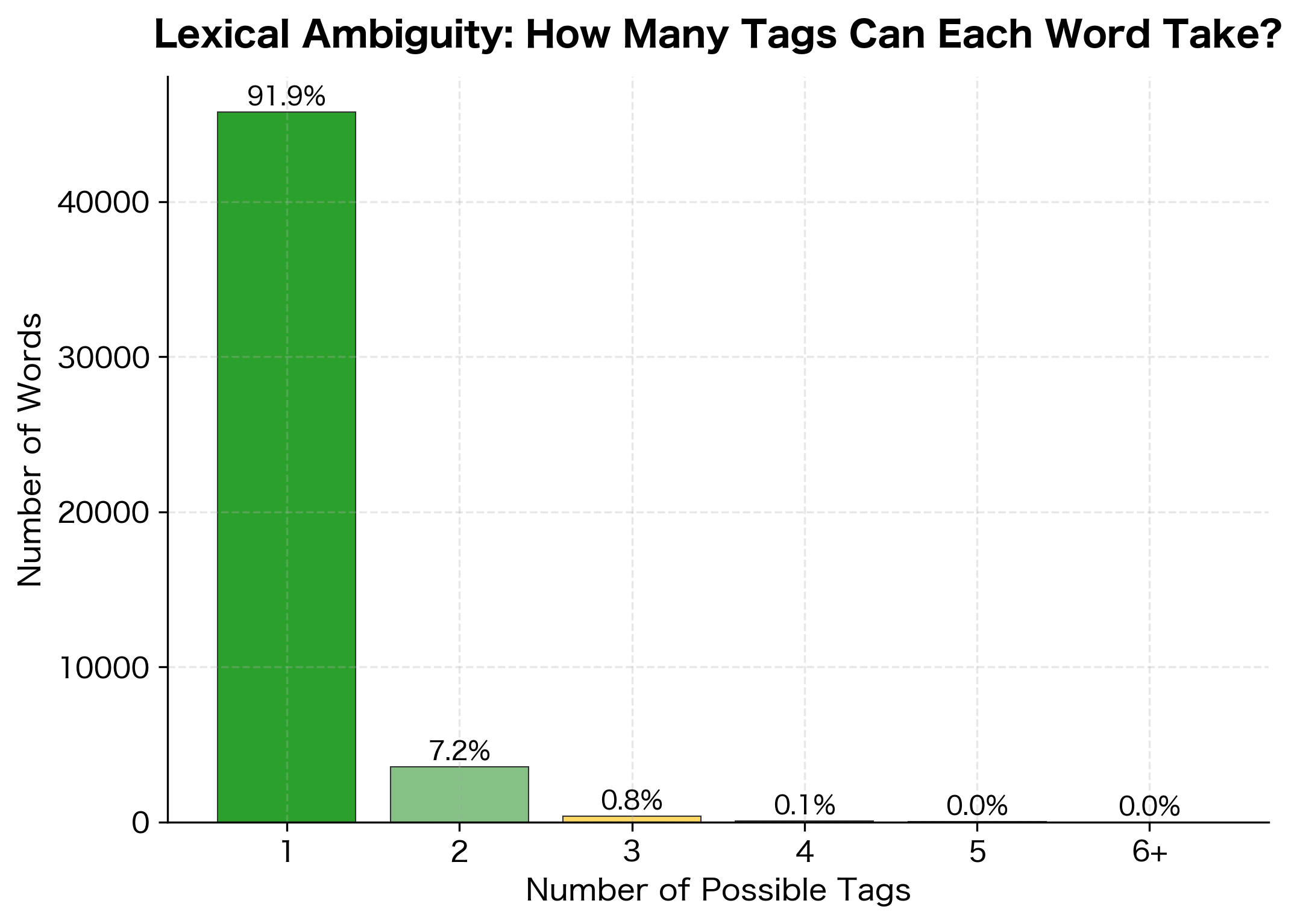
Studies of the Penn Treebank show that about 40% of word tokens are ambiguous, having multiple possible tags. However, context usually resolves the ambiguity. After seeing "the," we expect a noun or adjective, not a verb. After seeing "can," if the next word is a verb, then "can" is likely a modal.

Quantifying Ambiguity

Let's measure how much ambiguity exists in English text using the Brown corpus:

In[10]:
Code
import nltk
from collections import defaultdict

# Download required data
try:
    nltk.data.find("corpora/brown")
except LookupError:
    nltk.download("brown", quiet=True)

from nltk.corpus import brown

# Count tags for each word
word_tags = defaultdict(set)

for word, tag in brown.tagged_words():
    # Normalize: lowercase word, take first two chars of tag
    word_lower = word.lower()
    tag_simple = tag[:2] if len(tag) >= 2 else tag
    word_tags[word_lower].add(tag_simple)

# Analyze ambiguity
total_words = len(word_tags)
ambiguous_words = sum(1 for tags in word_tags.values() if len(tags) > 1)
highly_ambiguous = sum(1 for tags in word_tags.values() if len(tags) >= 3)
Out[11]:
Console
Ambiguity Analysis (Brown Corpus)
==================================================

Total unique words:       49,815
Ambiguous words (2+ tags): 4,029 (8.1%)
Highly ambiguous (3+ tags): 465 (0.9%)

Most ambiguous words:
  ':': 8 tags - ,, ., .-, :, :-, IN, NI, NP
  'down': 7 tags - IN, JJ, NN, NP, RB, RP, VB
  'well': 6 tags - JJ, NN, QL, RB, UH, VB
  'still': 6 tags - JJ, NN, NP, QL, RB, VB
  'that': 5 tags - CS, DT, NI, QL, WP
  'in': 5 tags - FW, IN, NI, NN, RP
  'to': 5 tags - IN, NI, NP, QL, TO
  'a': 5 tags - AT, FW, NI, NN, NP
  'best': 5 tags - JJ, NP, QL, RB, VB
  'as': 5 tags - CS, IN, NI, QL, RB

The analysis reveals that a significant portion of words can take multiple tags. However, frequency matters. Common words like "the" are unambiguous (always DT), while rarer words show more variation. The most ambiguous words often include function words and common verbs that double as nouns.

Out[12]:
Visualization
Bar chart showing the number of possible POS tags per word, with most words having 1 tag and decreasing counts for 2, 3, 4+ tags.
Distribution of lexical ambiguity in the Brown corpus. Most words are unambiguous (only one tag), but a substantial portion can take 2-3 tags depending on context. A small number of highly ambiguous words can take 4 or more tags.

Rule-Based POS Tagging

Before statistical methods dominated, researchers built rule-based taggers using hand-crafted patterns. While largely superseded, understanding these approaches provides intuition for what makes tagging difficult.

A Simple Pattern-Based Tagger

The simplest approach assigns tags based on word endings and patterns:

In[13]:
Code
import re


class PatternTagger:
    """A simple rule-based POS tagger using word patterns."""

    def __init__(self):
        # Default tag for unknown patterns
        self.default_tag = "NN"

        # Ordered list of (pattern, tag) rules
        self.rules = [
            # Punctuation
            (r"^[.!?]$", "."),
            (r"^[,;:]$", ","),
            (r"^[$]$", "$"),
            # Numbers
            (r"^-?\d+\.?\d*$", "CD"),
            (r"^\d+(?:st|nd|rd|th)$", "JJ"),
            # Verb endings
            (r".*ing$", "VBG"),  # running, eating
            (r".*ed$", "VBD"),  # walked, played
            (r".*es$", "VBZ"),  # goes, does
            (r".*ly$", "RB"),  # quickly, slowly
            # Adjective endings
            (r".*ful$", "JJ"),  # beautiful, helpful
            (r".*less$", "JJ"),  # careless, hopeless
            (r".*ous$", "JJ"),  # dangerous, famous
            (r".*ive$", "JJ"),  # active, creative
            (r".*able$", "JJ"),  # readable, capable
            (r".*ible$", "JJ"),  # visible, possible
            (r".*al$", "JJ"),  # natural, musical
            # Noun endings
            (r".*ness$", "NN"),  # happiness, darkness
            (r".*ment$", "NN"),  # movement, agreement
            (r".*tion$", "NN"),  # action, creation
            (r".*sion$", "NN"),  # decision, tension
            (r".*er$", "NN"),  # teacher, worker
            (r".*or$", "NN"),  # actor, director
        ]

        # Compile patterns
        self.compiled_rules = [(re.compile(p), t) for p, t in self.rules]

        # High-frequency word lookup
        self.lexicon = {
            "the": "DT",
            "a": "DT",
            "an": "DT",
            "is": "VBZ",
            "are": "VBP",
            "was": "VBD",
            "were": "VBD",
            "be": "VB",
            "been": "VBN",
            "being": "VBG",
            "have": "VBP",
            "has": "VBZ",
            "had": "VBD",
            "do": "VBP",
            "does": "VBZ",
            "did": "VBD",
            "will": "MD",
            "would": "MD",
            "could": "MD",
            "should": "MD",
            "may": "MD",
            "might": "MD",
            "must": "MD",
            "can": "MD",
            "i": "PRP",
            "you": "PRP",
            "he": "PRP",
            "she": "PRP",
            "it": "PRP",
            "we": "PRP",
            "they": "PRP",
            "this": "DT",
            "that": "DT",
            "these": "DT",
            "those": "DT",
            "and": "CC",
            "or": "CC",
            "but": "CC",
            "in": "IN",
            "on": "IN",
            "at": "IN",
            "to": "TO",
            "of": "IN",
            "for": "IN",
            "with": "IN",
            "by": "IN",
            "not": "RB",
            "very": "RB",
            "also": "RB",
        }

    def tag_word(self, word):
        """Tag a single word."""
        word_lower = word.lower()

        # Check lexicon first
        if word_lower in self.lexicon:
            return self.lexicon[word_lower]

        # Try pattern rules
        for pattern, tag in self.compiled_rules:
            if pattern.match(word_lower):
                return tag

        # Capitalized words might be proper nouns
        if word[0].isupper():
            return "NNP"

        return self.default_tag

    def tag(self, sentence):
        """Tag a sentence (list of words)."""
        return [(word, self.tag_word(word)) for word in sentence]

The PatternTagger applies rules in order: first checking a lexicon of common words with known tags, then matching suffix patterns, and finally falling back to defaults. This approach captures obvious cases but ignores context entirely.

In[14]:
Code
# Test the pattern tagger
tagger = PatternTagger()

test_sentences = [
    "The quick brown fox jumps over the lazy dog".split(),
    "She is running quickly through the beautiful garden".split(),
    "The teacher explained the confusing problem carefully".split(),
]

pattern_results = [tagger.tag(sent) for sent in test_sentences]
Out[15]:
Console
Pattern Tagger Results
============================================================

Input: The quick brown fox jumps over the lazy dog
Tagged: The/DT quick/NN brown/NN fox/NN jumps/NN over/NN the/DT lazy/NN dog/NN

Input: She is running quickly through the beautiful garden
Tagged: She/PRP is/VBZ running/VBG quickly/RB through/NN the/DT beautiful/JJ garden/NN

Input: The teacher explained the confusing problem carefully
Tagged: The/DT teacher/NN explained/VBD the/DT confusing/VBG problem/NN carefully/RB

The pattern tagger handles clear cases well: "quickly" gets RB due to the "-ly" suffix, "running" gets VBG due to "-ing", and "beautiful" gets JJ due to "-ful". However, it fails on ambiguous words where context matters.

Limitations of Patterns

Pattern-based taggers break down on contextual ambiguity:

In[16]:
Code
# Cases where patterns fail
failure_cases = [
    "I can fish".split(),  # can = MD, fish = VB
    "Open the can of fish".split(),  # can = NN, fish = NN
    "The fish can swim".split(),  # fish = NN, can = MD
]

pattern_failures = [tagger.tag(sent) for sent in failure_cases]
Out[17]:
Console
Pattern Tagger Failures
============================================================

Input: I can fish
Pattern: I/PRP can/MD fish/NN
Correct: I/PRP can/MD fish/VB
Errors: 1

Input: Open the can of fish
Pattern: Open/NNP the/DT can/MD of/IN fish/NN
Correct: Open/VB the/DT can/NN of/IN fish/NN
Errors: 2

Input: The fish can swim
Pattern: The/DT fish/NN can/MD swim/NN
Correct: The/DT fish/NN can/MD swim/VB
Errors: 1

The pattern tagger assigns "can" as MD (modal) in all cases because that's in its lexicon, but "can" should be NN when it's a container. Similarly, "fish" gets tagged as NN by default, but it's a verb in "I can fish." Resolving these cases requires examining surrounding words.

Using NLTK's Taggers

NLTK provides several pre-trained taggers that handle context and ambiguity:

In[18]:
Code
import nltk
from nltk import pos_tag, word_tokenize

# Download required resources
try:
    nltk.data.find("taggers/averaged_perceptron_tagger_eng")
except LookupError:
    nltk.download("averaged_perceptron_tagger_eng", quiet=True)

try:
    nltk.data.find("tokenizers/punkt_tab")
except LookupError:
    nltk.download("punkt_tab", quiet=True)

# Tag sentences
sentences_text = [
    "The quick brown fox jumps over the lazy dog.",
    "I can fish in the lake.",
    "Open the can of fish.",
    "The fish can swim fast.",
]

nltk_results = []
for sent in sentences_text:
    tokens = word_tokenize(sent)
    tagged = pos_tag(tokens)
    nltk_results.append((sent, tagged))
Out[19]:
Console
NLTK POS Tagger Results
============================================================

Input: The quick brown fox jumps over the lazy dog.
Tagged: The/DT quick/JJ brown/NN fox/NN jumps/VBZ over/IN the/DT lazy/JJ dog/NN ./.

Input: I can fish in the lake.
Tagged: I/PRP can/MD fish/VB in/IN the/DT lake/NN ./.

Input: Open the can of fish.
Tagged: Open/VB the/DT can/MD of/IN fish/NN ./.

Input: The fish can swim fast.
Tagged: The/DT fish/NN can/MD swim/VB fast/RB ./.

NLTK's default tagger is an averaged perceptron model trained on the Penn Treebank. It uses features from the current word, surrounding words, and previously predicted tags to make contextually informed decisions. Notice how it correctly handles "can" as both a modal verb and a noun depending on context.

Tagset Conversion with NLTK

NLTK can also convert to Universal tags:

In[20]:
Code
from nltk.tag import map_tag


def tag_with_universal(sentence):
    """Tag with Penn Treebank and convert to Universal."""
    tokens = word_tokenize(sentence)
    ptb_tagged = pos_tag(tokens)

    universal_tagged = [
        (word, map_tag("en-ptb", "universal", tag)) for word, tag in ptb_tagged
    ]
    return ptb_tagged, universal_tagged


sample = "The quick brown fox jumps over the lazy dog."
ptb_tags, universal_tags = tag_with_universal(sample)
Out[21]:
Console
Tagset Comparison
============================================================

Sentence: The quick brown fox jumps over the lazy dog.

Penn Treebank tags:
  The/DT quick/JJ brown/NN fox/NN jumps/VBZ over/IN the/DT lazy/JJ dog/NN ./.

Universal tags:
  The/DET quick/ADJ brown/NOUN fox/NOUN jumps/VERB over/ADP the/DET lazy/ADJ dog/NOUN ./.

Using spaCy's Tagger

spaCy provides fast, accurate tagging with both fine-grained and coarse tags:

In[22]:
Code
import spacy

# Load the English model
try:
    nlp = spacy.load("en_core_web_sm")
except OSError:
    # If model not installed, download it
    import subprocess

    subprocess.run(
        ["python", "-m", "spacy", "download", "en_core_web_sm"],
        capture_output=True,
    )
    nlp = spacy.load("en_core_web_sm")

# Process sentences
spacy_sentences = [
    "The quick brown fox jumps over the lazy dog.",
    "She can run faster than he can.",
    "Time flies like an arrow; fruit flies like a banana.",
]

spacy_results = []
for sent in spacy_sentences:
    doc = nlp(sent)
    tokens = [(token.text, token.tag_, token.pos_) for token in doc]
    spacy_results.append((sent, tokens))
Out[23]:
Console
spaCy POS Tagging
============================================================

Input: The quick brown fox jumps over the lazy dog.

  Token        Fine     Coarse
  -----------------------------------
  The          DT       DET
  quick        JJ       ADJ
  brown        JJ       ADJ
  fox          NN       NOUN
  jumps        VBZ      VERB
  over         IN       ADP
  the          DT       DET
  lazy         JJ       ADJ
  dog          NN       NOUN
  .            .        PUNCT

Input: She can run faster than he can.

  Token        Fine     Coarse
  -----------------------------------
  She          PRP      PRON
  can          MD       AUX
  run          VB       VERB
  faster       RBR      ADV
  than         IN       SCONJ
  he           PRP      PRON
  can          MD       AUX
  .            .        PUNCT

Input: Time flies like an arrow; fruit flies like a banana.

  Token        Fine     Coarse
  -----------------------------------
  Time         NN       NOUN
  flies        VBZ      VERB
  like         IN       ADP
  an           DT       DET
  arrow        NN       NOUN
  ;            :        PUNCT
  fruit        NN       NOUN
  flies        NNS      NOUN
  like         IN       ADP
  a            DT       DET
  banana       NN       NOUN
  .            .        PUNCT

spaCy provides both fine-grained tags (like Penn Treebank's VBZ) and coarse Universal tags. The token.tag_ attribute gives fine-grained tags while token.pos_ gives Universal tags. This dual annotation is convenient when you need different levels of granularity.

Explaining Tags

spaCy includes explanations for each tag:

In[24]:
Code
# Get explanations for tags
common_tags = [
    "NN",
    "NNS",
    "NNP",
    "VB",
    "VBD",
    "VBG",
    "VBZ",
    "JJ",
    "RB",
    "DT",
    "IN",
]
tag_explanations = {tag: spacy.explain(tag) for tag in common_tags}
Out[25]:
Console
Tag Explanations (spaCy)
==================================================
  NN    - noun, singular or mass
  NNS   - noun, plural
  NNP   - noun, proper singular
  VB    - verb, base form
  VBD   - verb, past tense
  VBG   - verb, gerund or present participle
  VBZ   - verb, 3rd person singular present
  JJ    - adjective (English), other noun-modifier (Chinese)
  RB    - adverb
  DT    - determiner
  IN    - conjunction, subordinating or preposition

Building a Statistical Tagger

The pattern-based tagger we built earlier fails on ambiguous words because it ignores context. To do better, we need a tagger that learns from data which tags are likely for each word and, crucially, which tags tend to follow other tags. This section walks through building such a tagger from scratch, developing the mathematical intuition step by step.

The Core Insight: Words and Sequences Both Matter

Imagine you encounter the word "can" in a sentence. How do you decide if it's a modal verb ("She can swim") or a noun ("Open the can")? You use two types of evidence:

  1. Word-level evidence: Some words strongly prefer certain tags. "Quickly" is almost always an adverb. "The" is always a determiner. But "can" is genuinely ambiguous.

  2. Sequence-level evidence: Tags follow patterns. After "the," you expect a noun or adjective. After a modal verb like "can," you expect another verb. These grammatical regularities help disambiguate.

A statistical tagger captures both types of evidence as probability distributions learned from annotated training data.

Emission Probabilities: Linking Words to Tags

The first distribution answers: "Given that I know the tag, how likely is this particular word?" This is called the emission probability because we think of the tag as "emitting" or generating the word we observe.

Emission Probability

The emission probability P(wordtag)P(\text{word} | \text{tag}) measures how likely a specific word is to appear with a given part-of-speech tag. High emission probability means the word is typical for that tag.

Consider the tag NOUN. Words like "cat," "dog," "table," and "government" frequently appear as nouns, so they have high emission probability given the NOUN tag. The word "quickly," by contrast, almost never appears as a noun, so P(quicklyNOUN)P(\text{quickly} | \text{NOUN}) is nearly zero.

We estimate emission probabilities by counting how often each word appears with each tag in our training corpus, then normalizing:

P(wordtag)=C(word,tag)C(tag)P(\text{word} | \text{tag}) = \frac{C(\text{word}, \text{tag})}{C(\text{tag})}

where:

  • C(word,tag)C(\text{word}, \text{tag}): the count of times this word appeared with this tag in training
  • C(tag)C(\text{tag}): the total count of this tag across all words

For example, if "dog" appears 50 times with the NN tag in training, and NN appears 10,000 times total, then P(dogNN)=50/10000=0.005P(\text{dog} | \text{NN}) = 50 / 10000 = 0.005.

Transition Probabilities: Capturing Grammar

The second distribution captures sequential patterns: "Given the previous tag, how likely is the current tag?" This is called the transition probability because it describes how we transition from one tag to the next.

Transition Probability

The transition probability P(tagitagi1)P(\text{tag}_i | \text{tag}_{i-1}) measures how likely a tag is to follow another tag. High transition probability indicates a common grammatical pattern.

where:

  • tagi\text{tag}_i: the tag at position ii in the sentence
  • tagi1\text{tag}_{i-1}: the tag at the previous position

Some transitions are very common: determiners (DT) almost always precede nouns (NN) or adjectives (JJ). Other transitions are rare: you rarely see two determiners in a row. By learning these patterns from data, the tagger can use context to disambiguate.

We estimate transition probabilities similarly to emissions:

P(tagitagi1)=C(tagi1,tagi)C(tagi1)P(\text{tag}_i | \text{tag}_{i-1}) = \frac{C(\text{tag}_{i-1}, \text{tag}_i)}{C(\text{tag}_{i-1})}

where:

  • C(tagi1,tagi)C(\text{tag}_{i-1}, \text{tag}_i): the count of times tagi\text{tag}_i immediately followed tagi1\text{tag}_{i-1}
  • C(tagi1)C(\text{tag}_{i-1}): the total count of tagi1\text{tag}_{i-1} in the corpus

Combining Evidence: The Scoring Function

Now we can score candidate tags by combining both types of evidence. For a word at position ii with previous tag tagi1\text{tag}_{i-1}, we want to find the tag that maximizes:

score(tagi)=P(worditagi)×P(tagitagi1)\text{score}(\text{tag}_i) = P(\text{word}_i | \text{tag}_i) \times P(\text{tag}_i | \text{tag}_{i-1})

This product captures both how well the tag explains the word (emission) and how well it fits the grammatical context (transition). The tag with the highest combined score wins.

In practice, we work in log space to avoid numerical underflow when multiplying many small probabilities:

score(tagi)=logP(worditagi)+logP(tagitagi1)\text{score}(\text{tag}_i) = \log P(\text{word}_i | \text{tag}_i) + \log P(\text{tag}_i | \text{tag}_{i-1})

where logarithms convert the multiplication to addition, making computation more stable.

Implementation

Let's implement this statistical tagger step by step:

In[26]:
Code
from collections import Counter, defaultdict


class SimpleStatisticalTagger:
    """A statistical POS tagger using emission and transition probabilities."""

    def __init__(self):
        # Emission counts: P(word | tag)
        self.word_tag_counts = defaultdict(Counter)
        self.tag_counts = Counter()

        # Transition counts: P(tag | prev_tag)
        self.transition_counts = defaultdict(Counter)
        self.prev_tag_counts = Counter()

        # Vocabulary
        self.vocabulary = set()
        self.tags = set()

    def train(self, tagged_sentences):
        """Learn probabilities from tagged training data."""
        for sentence in tagged_sentences:
            prev_tag = "<START>"
            for word, tag in sentence:
                # Emission counts
                word_lower = word.lower()
                self.word_tag_counts[tag][word_lower] += 1
                self.tag_counts[tag] += 1

                # Transition counts
                self.transition_counts[prev_tag][tag] += 1
                self.prev_tag_counts[prev_tag] += 1

                # Track vocabulary and tags
                self.vocabulary.add(word_lower)
                self.tags.add(tag)

                prev_tag = tag

            # End of sentence
            self.transition_counts[prev_tag]["<END>"] += 1
            self.prev_tag_counts[prev_tag] += 1

    def emission_prob(self, word, tag, smoothing=0.001):
        """P(word | tag) with add-k smoothing."""
        word_lower = word.lower()
        count = self.word_tag_counts[tag][word_lower]
        total = self.tag_counts[tag]
        vocab_size = len(self.vocabulary)

        return (count + smoothing) / (total + smoothing * vocab_size)

    def transition_prob(self, tag, prev_tag, smoothing=0.001):
        """P(tag | prev_tag) with add-k smoothing."""
        count = self.transition_counts[prev_tag][tag]
        total = self.prev_tag_counts[prev_tag]
        num_tags = len(self.tags)

        return (count + smoothing) / (total + smoothing * num_tags)

The train method iterates through tagged sentences, building four data structures:

  1. word_tag_counts: For each tag, counts how often each word appeared with that tag
  2. tag_counts: Total occurrences of each tag (for normalizing emission probabilities)
  3. transition_counts: For each previous tag, counts how often each current tag followed
  4. prev_tag_counts: Total occurrences of each tag as a predecessor (for normalizing transitions)

We also track the vocabulary and tag set, which we'll need during inference.

Handling Unseen Events: Smoothing

There's a critical problem with the raw probability estimates: any word-tag combination not seen in training gets probability zero. If the test data contains the word "smartphone" but our 1990s training data doesn't include it, the model can't assign any tag to it.

We solve this with add-k smoothing (also called Laplace smoothing), which adds a small constant to all counts:

P(wordtag)=C(word,tag)+kC(tag)+k×VP(\text{word} | \text{tag}) = \frac{C(\text{word}, \text{tag}) + k}{C(\text{tag}) + k \times |V|}

where:

  • C(word,tag)C(\text{word}, \text{tag}): the raw count of times this word appeared with this tag
  • C(tag)C(\text{tag}): the total count of this tag across all words
  • kk: the smoothing constant (we use 0.001), which adds a small probability mass to unseen events
  • V|V|: the vocabulary size, used to ensure probabilities sum to 1

The intuition is simple: instead of saying "I've never seen 'smartphone' as a noun, so probability is zero," we say "I've never seen it, but it's possible, so here's a tiny probability." The denominator adjustment ensures all probabilities still sum to 1.

Smaller kk values trust the training data more, while larger values spread probability more evenly across possibilities. A value of 0.001 works well in practice, keeping probabilities close to the empirical estimates while preventing zeros.

Greedy Decoding: Choosing Tags

With our probability estimates in hand, we need a strategy for choosing tags. The simplest approach is greedy decoding: at each position, pick the tag that maximizes the score, then move on:

In[27]:
Code
import math


def tag_greedy(self, words):
    """Tag using greedy decoding (pick best tag at each position)."""
    tagged = []
    prev_tag = "<START>"

    for word in words:
        best_tag = None
        best_score = float("-inf")

        for tag in self.tags:
            # Combine emission and transition probabilities (in log space)
            emission = math.log(self.emission_prob(word, tag) + 1e-10)
            transition = math.log(self.transition_prob(tag, prev_tag) + 1e-10)
            score = emission + transition

            if score > best_score:
                best_score = score
                best_tag = tag

        # Handle unknown words
        if best_tag is None:
            best_tag = "NN"  # Default to noun

        tagged.append((word, best_tag))
        prev_tag = best_tag

    return tagged


# Add method to class
SimpleStatisticalTagger.tag_greedy = tag_greedy

The greedy decoder loops through each word, computing a score for every possible tag by combining emission and transition probabilities. The implementation uses log probabilities for numerical stability, converting the multiplication in our scoring formula to addition:

score(tag)=logP(wordtag)+logP(tagprev_tag)\text{score}(\text{tag}) = \log P(\text{word} | \text{tag}) + \log P(\text{tag} | \text{prev\_tag})

where:

  • P(wordtag)P(\text{word} | \text{tag}): the emission probability, measuring how likely this word is given the proposed tag
  • P(tagprev_tag)P(\text{tag} | \text{prev\_tag}): the transition probability, measuring how likely this tag is given what came before

The tag with the highest combined score wins. We add a tiny constant (1e-10) before taking logarithms to avoid taking the log of zero.

Greedy decoding has an important limitation: it makes locally optimal choices that may be globally suboptimal. Consider the sentence "I can fish." When processing "can," the tagger doesn't yet know that "fish" follows. If the training data strongly associates "can" with the modal verb tag, greedy decoding picks that, even though the full context suggests "can" might be a verb in "I can [verb] fish" (meaning "I am able to fish").

More sophisticated approaches like the Viterbi algorithm (covered in a later chapter) consider all possible tag sequences simultaneously, finding the globally optimal path. But greedy decoding is fast and works reasonably well when transitions provide strong guidance.

Putting It Together: Training and Evaluation

Now let's train our statistical tagger on real data and see how it performs:

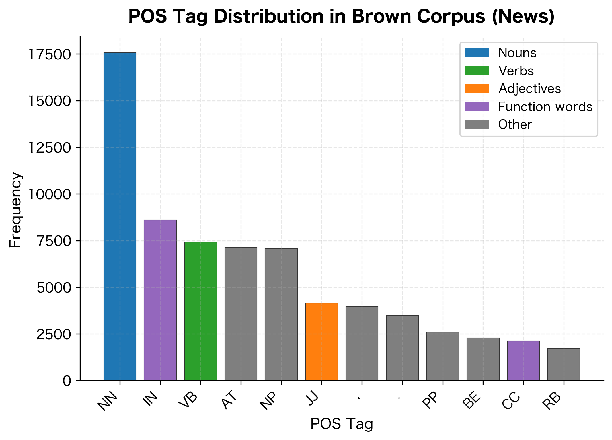
We'll use the Brown corpus, a classic collection of American English text from the 1960s, which includes POS annotations. We simplify the tags to their first two characters (e.g., "NN" and "NNS" both become "NN") to reduce the tag set size and make patterns easier to see:

In[28]:
Code
from nltk.corpus import brown

# Get tagged sentences
tagged_sents = brown.tagged_sents(categories="news")


# Simplify tags to first two characters
def simplify_tags(sentence):
    return [(word, tag[:2] if len(tag) >= 2 else tag) for word, tag in sentence]


simplified_sents = [simplify_tags(sent) for sent in tagged_sents]

# Split into train and test
split_point = int(len(simplified_sents) * 0.8)
train_sents = simplified_sents[:split_point]
test_sents = simplified_sents[split_point:]

# Train the tagger
stat_tagger = SimpleStatisticalTagger()
stat_tagger.train(train_sents)
Out[29]:
Console
Training Statistics
==================================================
Training sentences: 3,698
Test sentences: 925
Vocabulary size: 11,423
Number of tags: 46

Most frequent tags:
  NN  : 17,561
  IN  : 8,599
  VB  : 7,423
  AT  : 7,125
  NP  : 7,072
  JJ  : 4,154
  ,   : 3,975
  .   : 3,500
  PP  : 2,590
  BE  : 2,281

The training data contains several thousand sentences with a vocabulary of thousands of unique words. The tag distribution is heavily skewed: nouns (NN) and prepositions (IN) dominate, reflecting their prevalence in news text. Less common tags like modal verbs (MD) and conjunctions (CC) appear far less frequently but are important for grammatical structure.

This skewed distribution has implications for our tagger. Tags with more training examples will have more reliable probability estimates, while rare tags may suffer from sparse data.

Measuring Performance

To evaluate our tagger, we compare its predictions against the gold-standard annotations in our test set. We compute overall accuracy (percentage of tokens tagged correctly) and per-tag accuracy to identify which categories are harder:

In[30]:
Code
def evaluate_tagger(tagger, test_sentences, tag_method="tag_greedy"):
    """Evaluate tagger accuracy on test sentences."""
    correct = 0
    total = 0

    # Track errors by tag
    tag_errors = defaultdict(lambda: {"correct": 0, "total": 0})
    confusion = defaultdict(Counter)

    tag_func = getattr(tagger, tag_method)

    for sentence in test_sentences:
        words = [word for word, tag in sentence]
        gold_tags = [tag for word, tag in sentence]

        predicted = tag_func(words)
        pred_tags = [tag for word, tag in predicted]

        for gold, pred in zip(gold_tags, pred_tags):
            total += 1
            tag_errors[gold]["total"] += 1

            if gold == pred:
                correct += 1
                tag_errors[gold]["correct"] += 1
            else:
                confusion[gold][pred] += 1

    accuracy = correct / total if total > 0 else 0

    # Per-tag accuracy
    per_tag_accuracy = {}
    for tag, counts in tag_errors.items():
        if counts["total"] > 0:
            per_tag_accuracy[tag] = counts["correct"] / counts["total"]

    return {
        "accuracy": accuracy,
        "correct": correct,
        "total": total,
        "per_tag": per_tag_accuracy,
        "confusion": confusion,
    }


results = evaluate_tagger(stat_tagger, test_sents)
Out[31]:
Console
Tagger Evaluation
==================================================

Overall Accuracy: 83.66%
Correct: 17,367 / 20,759

Per-Tag Accuracy (top 10 tags):
  NN  : 77.2% (17,561 examples)
  IN  : 90.6% (8,599 examples)
  VB  : 74.1% (7,423 examples)
  AT  : 99.2% (7,125 examples)
  NP  : 59.2% (7,072 examples)
  JJ  : 66.2% (4,154 examples)
  ,   : 100.0% (3,975 examples)
  .   : 99.4% (3,500 examples)
  PP  : 97.4% (2,590 examples)
  BE  : 99.3% (2,281 examples)
Out[32]:
Visualization
Horizontal bar chart showing accuracy for different POS tag categories, with function words achieving highest accuracy.
Accuracy breakdown by POS tag category. Closed-class words like determiners (AT) and prepositions (IN) achieve near-perfect accuracy due to their limited, predictable behavior. Open-class words like nouns (NN) and verbs (VB) are harder because they include many ambiguous members.

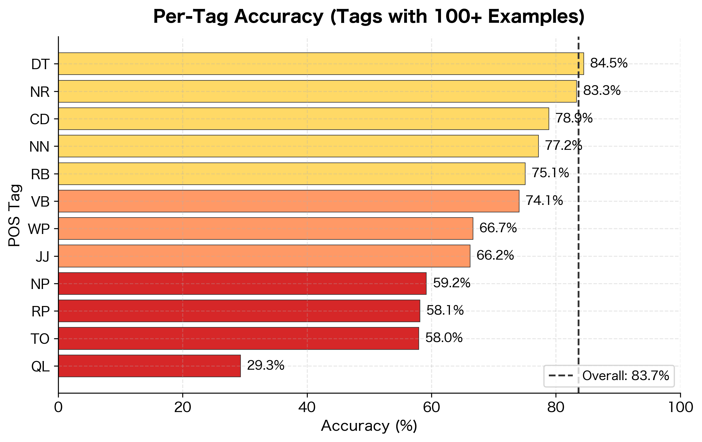
Our simple statistical tagger achieves reasonable accuracy, demonstrating that even a straightforward probabilistic approach outperforms pattern-based rules. The per-tag breakdown reveals an interesting pattern: closed-class words like determiners (DT) and prepositions (IN) achieve high accuracy because they have limited, predictable behavior. Open-class words like nouns (NN) and verbs (VB) are harder because they include many ambiguous words and the categories are more diverse.

The accuracy is respectable but falls short of state-of-the-art systems (97%+). The gap comes from several sources: our greedy decoding misses some context, our simplified tag set loses information, and we don't use morphological features beyond the word itself.

Understanding Errors

Looking at where the tagger fails reveals systematic patterns that suggest improvements:

In[33]:
Code
# Find most common confusions
all_confusions = []
for gold_tag, pred_counts in results["confusion"].items():
    for pred_tag, count in pred_counts.items():
        all_confusions.append((gold_tag, pred_tag, count))

top_confusions = sorted(all_confusions, key=lambda x: -x[2])[:10]
Out[34]:
Console
Most Common Tagging Errors
==================================================

  Gold → Predicted  Count
  ------------------------------
  NN   → OD         205
  JJ   → OD         139
  TO   → IN         120
  VB   → NN         105
  NP   → OD         100
  IN   → TO         96
  NN   → AT         96
  VB   → *          91
  NN   → VB         74
  NP   → AT         70
Out[35]:
Visualization
Heatmap confusion matrix showing which POS tags are most commonly confused with each other.
Confusion matrix showing tagging errors for the most frequent tags. Darker cells indicate more errors. The NN-NP confusion (common nouns vs. proper nouns) is the dominant error pattern, followed by adjective-noun and verb-form confusions.

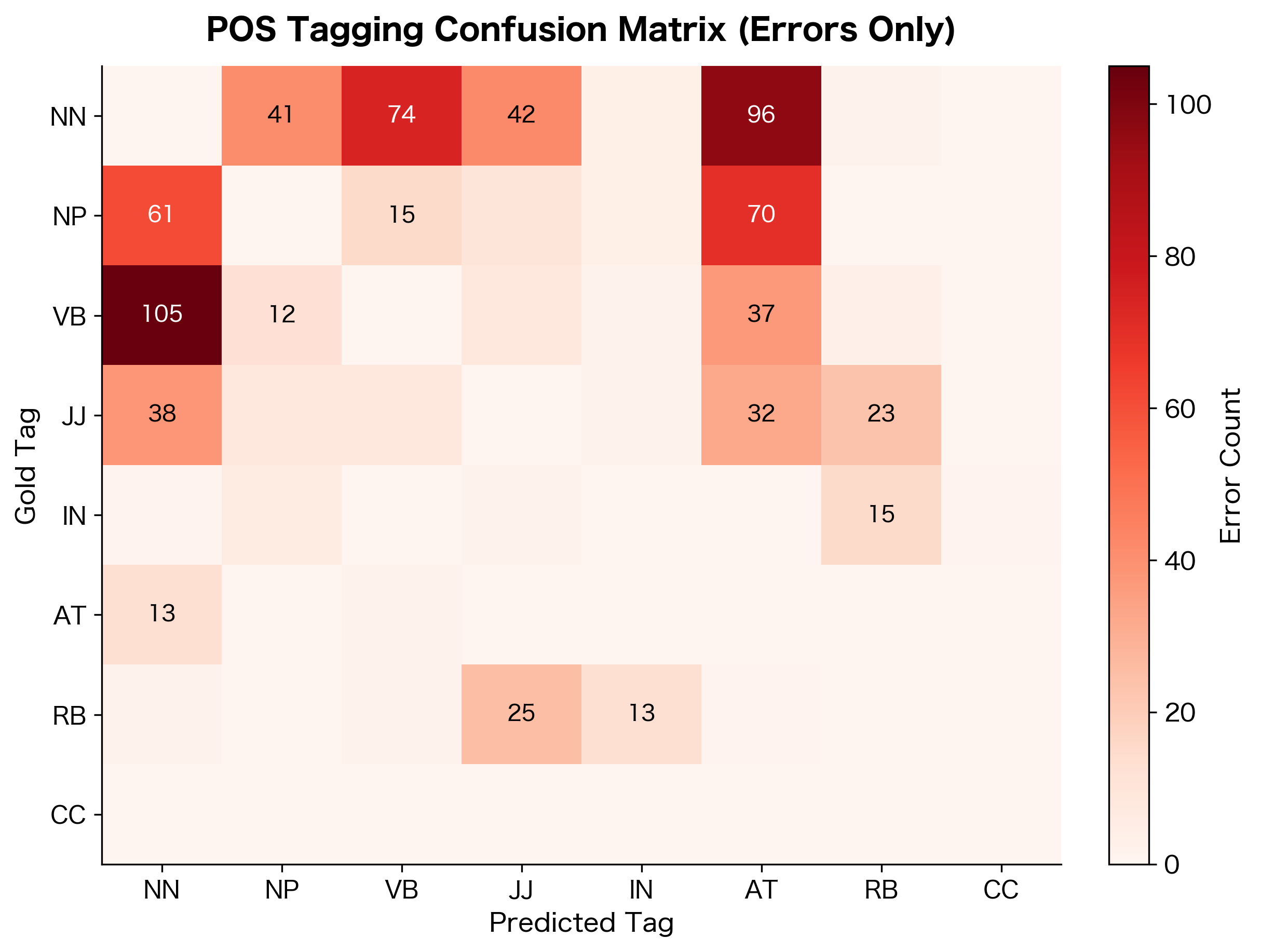
The error analysis reveals systematic confusion patterns. Nouns and proper nouns (NN vs. NP) are frequently confused because capitalization is the primary distinguishing feature, and our tagger doesn't use that signal effectively. Adjectives and nouns (JJ vs. NN) cause trouble because many English words can serve both functions ("the stone wall" vs. "throw the stone"). Verb form confusions (VB vs. VBD) often involve irregular verbs where past tense isn't marked by the "-ed" suffix.

Evaluation Metrics for POS Tagging

Accuracy, the percentage of correctly tagged tokens, is the standard metric for POS tagging. However, several nuances matter in practice.

POS Tagging Accuracy

POS tagging accuracy measures the percentage of tokens assigned the correct tag. Modern taggers achieve 97%+ accuracy on standard benchmarks, but performance varies significantly across text types and tag categories.

Known vs. Unknown Words

A critical distinction in evaluation is between known words (seen in training) and unknown words (out-of-vocabulary, OOV). Taggers typically perform much better on known words:

In[36]:
Code
def evaluate_by_word_type(tagger, test_sentences, training_vocab):
    """Separate evaluation for known and unknown words."""
    known_correct, known_total = 0, 0
    unknown_correct, unknown_total = 0, 0

    for sentence in test_sentences:
        words = [word for word, tag in sentence]
        gold_tags = [tag for word, tag in sentence]

        predicted = tagger.tag_greedy(words)

        for (word, gold), (_, pred) in zip(sentence, predicted):
            is_known = word.lower() in training_vocab

            if is_known:
                known_total += 1
                if gold == pred:
                    known_correct += 1
            else:
                unknown_total += 1
                if gold == pred:
                    unknown_correct += 1

    return {
        "known_accuracy": known_correct / known_total if known_total > 0 else 0,
        "unknown_accuracy": unknown_correct / unknown_total
        if unknown_total > 0
        else 0,
        "known_total": known_total,
        "unknown_total": unknown_total,
    }


word_type_results = evaluate_by_word_type(
    stat_tagger, test_sents, stat_tagger.vocabulary
)
Out[37]:
Console
Accuracy by Word Type
==================================================

Known words:
  Accuracy: 93.19%
  Count: 18,452

Unknown words:
  Accuracy: 7.46%
  Count: 2,307

OOV rate: 11.1%
Accuracy gap: 85.7%

The gap between known and unknown word accuracy is substantial, as summarized in the table below. For unknown words, taggers must rely on morphological patterns, context, and default rules. This is why suffix-based rules (like assigning VBG to words ending in "-ing") remain useful even in statistical systems.

Out[38]:
Console
| Word Type | Accuracy | Count |
|:----------|:--------:|------:|
| Known words | 93.2% | 18,452 |
| Unknown words | 7.5% | 2,307 |
| **Accuracy gap** | **85.7%** | — |

: Accuracy comparison between known and unknown words. The substantial gap highlights the challenge of handling novel words. {#tbl-known-unknown-accuracy}

Sentence-Level Accuracy

Another perspective is sentence-level accuracy: the percentage of sentences where every word is tagged correctly:

In[39]:
Code
def sentence_accuracy(tagger, test_sentences):
    """Calculate percentage of perfectly tagged sentences."""
    perfect = 0
    total = len(test_sentences)

    for sentence in test_sentences:
        words = [word for word, tag in sentence]
        gold_tags = [tag for word, tag in sentence]

        predicted = tagger.tag_greedy(words)
        pred_tags = [tag for word, tag in predicted]

        if gold_tags == pred_tags:
            perfect += 1

    return perfect / total if total > 0 else 0


sent_acc = sentence_accuracy(stat_tagger, test_sents)
Out[40]:
Console
Sentence-Level Accuracy
==================================================

Perfect sentences: 9.1%
Token accuracy: 83.7%

(With 84% token accuracy, expect ~17% of 10-word sentences to be perfect)

Sentence-level accuracy is much lower than token accuracy because errors compound. If each token has probability pp of being correct and we assume independent errors, a sentence of nn words has probability pnp^n of being entirely correct. With 95% token accuracy, a 10-word sentence has only:

P(perfect sentence)=pn=0.95100.60P(\text{perfect sentence}) = p^n = 0.95^{10} \approx 0.60

where:

  • pp: the token-level accuracy (probability of correctly tagging a single word)
  • nn: the number of words in the sentence

This means roughly 40% of 10-word sentences contain at least one error, even with a highly accurate tagger. This matters for downstream tasks that process entire sentences, where a single tagging error can cascade into larger problems.

POS Tagging for Downstream Tasks

POS tags serve as features or preprocessing for many NLP tasks.

Information Extraction

POS patterns help identify entities and relations:

In[41]:
Code
def find_noun_phrases(tagged_sentence):
    """Find simple noun phrases using POS patterns."""
    # Pattern: (DT)? (JJ)* (NN|NNS|NNP|NNPS)+
    phrases = []
    current_phrase = []

    for word, tag in tagged_sentence:
        if tag in ("DT",) or tag.startswith("JJ") or tag.startswith("NN"):
            current_phrase.append((word, tag))
        else:
            if current_phrase:
                # Check if phrase ends with a noun
                last_tag = current_phrase[-1][1]
                if last_tag.startswith("NN"):
                    phrases.append(current_phrase)
                current_phrase = []

    # Handle phrase at end of sentence
    if current_phrase:
        last_tag = current_phrase[-1][1]
        if last_tag.startswith("NN"):
            phrases.append(current_phrase)

    return phrases


# Example
sample_text = "The quick brown fox jumps over the lazy dog."
sample_tagged = pos_tag(word_tokenize(sample_text))
noun_phrases = find_noun_phrases(sample_tagged)
Out[42]:
Console
Noun Phrase Extraction
==================================================

Sentence: The quick brown fox jumps over the lazy dog.

Tagged: The/DT quick/JJ brown/NN fox/NN jumps/VBZ over/IN the/DT lazy/JJ dog/NN ./.

Noun phrases found:
  'The quick brown fox' (DT JJ NN NN)
  'the lazy dog' (DT JJ NN)

Text Simplification

POS tags help identify which words to simplify:

In[43]:
Code
def count_pos_distribution(text):
    """Analyze POS distribution in text."""
    tokens = word_tokenize(text)
    tagged = pos_tag(tokens)

    # Group by major category
    categories = defaultdict(int)
    for word, tag in tagged:
        if tag.startswith("NN"):
            categories["Nouns"] += 1
        elif tag.startswith("VB"):
            categories["Verbs"] += 1
        elif tag.startswith("JJ"):
            categories["Adjectives"] += 1
        elif tag.startswith("RB"):
            categories["Adverbs"] += 1
        elif tag in ("DT", "IN", "CC", "TO"):
            categories["Function words"] += 1
        else:
            categories["Other"] += 1

    total = sum(categories.values())
    return {cat: (count, count / total) for cat, count in categories.items()}


# Compare two texts
technical = """
The implementation utilizes a sophisticated algorithm that incorporates 
machine learning techniques to optimize computational efficiency.
"""

simple = """
We made a program that learns from examples. It works fast.
"""

tech_dist = count_pos_distribution(technical)
simple_dist = count_pos_distribution(simple)
Out[44]:
Console
POS Distribution Comparison
============================================================

Technical text:
  "The implementation utilizes a sophisticated algorithm that i..."
    Nouns          :  5 (31.2%)
    Verbs          :  4 (25.0%)
    Function words :  3 (18.8%)
    Adjectives     :  2 (12.5%)
    Other          :  2 (12.5%)

Simple text:
  "We made a program that learns from examples. It works fast...."
    Other          :  5 (38.5%)
    Verbs          :  3 (23.1%)
    Function words :  2 (15.4%)
    Nouns          :  2 (15.4%)
    Adverbs        :  1 ( 7.7%)

Technical writing tends to have higher noun density (nominalization), while simpler writing uses more verbs. POS analysis helps identify these stylistic differences.

Visualizing POS Patterns

Visualizations help reveal the structure of tagged corpora. The following figures show POS tag frequency distributions and transition patterns from our trained statistical tagger, illustrating the grammatical regularities that make statistical tagging possible.

Out[45]:
Visualization
Bar chart showing POS tag frequencies with nouns most frequent, followed by prepositions, determiners, and verbs.
Distribution of part-of-speech categories in the Brown corpus news section. Nouns dominate, followed by prepositions and determiners. The high frequency of function words (determiners, prepositions, conjunctions) reflects their role as grammatical glue in English sentences.
Out[46]:
Visualization
Heatmap showing POS tag transition probabilities with darker cells indicating higher probability.
Transition probabilities between POS tags. Each cell shows how likely a tag (y-axis) is to follow another tag (x-axis). Strong patterns emerge: determiners almost always precede nouns or adjectives, and verbs are often followed by determiners, prepositions, or other verbs.

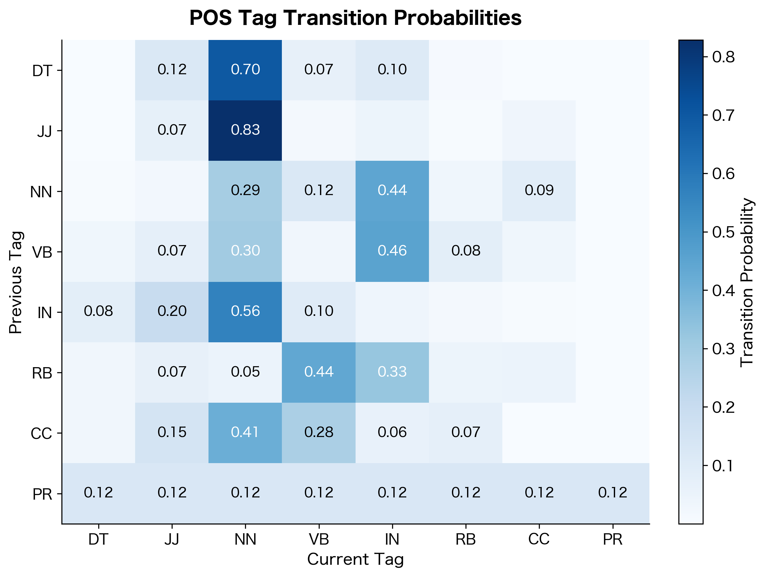
The transition matrix reveals grammatical patterns. Determiners (DT) strongly predict nouns (NN) or adjectives (JJ). Prepositions (IN) are often followed by determiners. These patterns reflect the syntactic structure of English.

Limitations and Challenges

Despite achieving high accuracy on benchmarks, POS tagging faces several ongoing challenges.

Domain shift causes significant accuracy drops when taggers trained on news text are applied to social media, scientific articles, or historical documents. Each domain has its own vocabulary, style, and even grammatical conventions. A tagger trained on formal news articles may struggle with the informal, abbreviated language of Twitter.

Rare and novel words pose difficulties because taggers have limited information for words seen infrequently or not at all during training. Technical jargon, proper nouns, and neologisms require inference from context and morphology rather than memorized patterns.

Annotation inconsistencies in training data propagate to learned models. Even expert annotators disagree on edge cases, particularly for words that can function as multiple parts of speech. The Penn Treebank guidelines span hundreds of pages precisely because many tagging decisions are genuinely ambiguous.

Cross-linguistic challenges arise because tag sets and grammatical categories vary across languages. What constitutes a "verb" differs between English, which marks tense morphologically, and Chinese, which uses aspectual particles. Universal Dependencies aims to address this but inevitably loses language-specific distinctions.

Error propagation affects downstream tasks that rely on POS tags. A 97% accurate tagger still makes errors on roughly 3% of tokens. For a document with 1000 words, that's 30 errors that propagate to dependency parsing, named entity recognition, or information extraction. These errors compound as documents get longer.

Impact on NLP

Part-of-speech tagging was among the first NLP tasks to achieve near-human performance through machine learning, demonstrating that statistical methods could capture linguistic patterns effectively. The transition from rule-based systems to statistical taggers in the 1990s influenced the broader shift toward data-driven approaches in the field.

The task has served as a proving ground for sequence labeling techniques. Hidden Markov Models, Maximum Entropy Markov Models, Conditional Random Fields, and more recently neural architectures were all benchmarked on POS tagging before being applied to more complex tasks.

Modern pre-trained language models like BERT often include POS tagging as an auxiliary objective or evaluation task. Interestingly, these models achieve superhuman accuracy on standard benchmarks, revealing that earlier accuracy ceilings reflected annotation noise rather than true task difficulty.

POS tags remain useful features even in the age of deep learning. They provide linguistically meaningful abstractions that can improve sample efficiency, particularly for low-resource languages or specialized domains. When you have limited training data, incorporating POS information can help models generalize better.

Key Functions and Parameters

When working with POS tagging in Python, these are the essential functions and their key parameters:

NLTK POS Tagging

nltk.pos_tag(tokens, tagset=None, lang='eng') tags a list of tokens with POS labels:

  • tokens: List of word strings to tag (typically from word_tokenize())
  • tagset: Target tagset. Use 'universal' for cross-linguistic Universal tags, or omit for Penn Treebank tags
  • lang: Language code for the tagger model. Default 'eng' works for English; other languages require downloading additional models

nltk.tag.map_tag(source, target, source_tag) converts between tag sets:

  • source: Source tagset identifier (e.g., 'en-ptb' for Penn Treebank)
  • target: Target tagset identifier (e.g., 'universal' for Universal Dependencies)
  • source_tag: The tag string to convert

spaCy POS Tagging

spacy.load(model_name) loads a pre-trained language model:

  • model_name: Model identifier like 'en_core_web_sm' (small), 'en_core_web_md' (medium), or 'en_core_web_lg' (large). Larger models are more accurate but slower and require more memory

After processing text with nlp(text), access POS information via token attributes:

  • token.pos_: Coarse-grained Universal POS tag (17 tags)
  • token.tag_: Fine-grained Penn Treebank-style tag (50+ tags)
  • spacy.explain(tag): Returns a human-readable explanation of any tag

Statistical Tagger Parameters

When building custom taggers, key parameters include:

  • smoothing: Add-k smoothing constant (typically 0.001 to 0.1). Higher values assign more probability to unseen events, reducing overfitting but potentially hurting accuracy on known words
  • train/test split: Standard practice uses 80-90% for training. Larger training sets improve accuracy, especially for rare words and tag transitions

Summary

Part-of-speech tagging assigns grammatical labels to words based on their function in context. The task appears simple but requires handling widespread ambiguity, where the same word form can serve as different parts of speech.

Key takeaways:

  • Tag sets define the inventory of labels. Penn Treebank uses 36 fine-grained tags while Universal Dependencies uses 17 cross-linguistic tags
  • Ambiguity affects roughly 40% of word tokens in English, requiring contextual disambiguation
  • Rule-based taggers use patterns and lexicons but fail on context-dependent ambiguity
  • Statistical taggers learn from annotated data, combining word features with transition patterns
  • NLTK and spaCy provide pre-trained taggers achieving 97%+ accuracy on standard benchmarks
  • Evaluation distinguishes between known and unknown words, with OOV words being significantly harder
  • Downstream applications use POS tags for noun phrase extraction, information extraction, and stylistic analysis

Part-of-speech tagging exemplifies a core NLP pattern: a task that seems trivial until you examine edge cases, where statistical methods substantially outperform hand-crafted rules, and where high but imperfect accuracy has real consequences for downstream processing.

Quiz

Ready to test your understanding? Take this quick quiz to reinforce what you've learned about part-of-speech tagging.

Loading component...

Comments

Reference

BIBTEXAcademic
@misc{partofspeechtaggingtagsetsalgorithmsimplementation, author = {Michael Brenndoerfer}, title = {Part-of-Speech Tagging: Tag Sets, Algorithms & Implementation}, year = {2025}, url = {https://mbrenndoerfer.com/writing/part-of-speech-tagging-nlp-guide}, organization = {mbrenndoerfer.com}, note = {Accessed: 2025-12-15} }
APAAcademic
Michael Brenndoerfer (2025). Part-of-Speech Tagging: Tag Sets, Algorithms & Implementation. Retrieved from https://mbrenndoerfer.com/writing/part-of-speech-tagging-nlp-guide
MLAAcademic
Michael Brenndoerfer. "Part-of-Speech Tagging: Tag Sets, Algorithms & Implementation." 2025. Web. 12/15/2025. <https://mbrenndoerfer.com/writing/part-of-speech-tagging-nlp-guide>.
CHICAGOAcademic
Michael Brenndoerfer. "Part-of-Speech Tagging: Tag Sets, Algorithms & Implementation." Accessed 12/15/2025. https://mbrenndoerfer.com/writing/part-of-speech-tagging-nlp-guide.
HARVARDAcademic
Michael Brenndoerfer (2025) 'Part-of-Speech Tagging: Tag Sets, Algorithms & Implementation'. Available at: https://mbrenndoerfer.com/writing/part-of-speech-tagging-nlp-guide (Accessed: 12/15/2025).
SimpleBasic
Michael Brenndoerfer (2025). Part-of-Speech Tagging: Tag Sets, Algorithms & Implementation. https://mbrenndoerfer.com/writing/part-of-speech-tagging-nlp-guide
Michael Brenndoerfer

About the author: Michael Brenndoerfer

All opinions expressed here are my own and do not reflect the views of my employer.

Michael currently works as an Associate Director of Data Science at EQT Partners in Singapore, leading AI and data initiatives across private capital investments.

With over a decade of experience spanning private equity, management consulting, and software engineering, he specializes in building and scaling analytics capabilities from the ground up. He has published research in leading AI conferences and holds expertise in machine learning, natural language processing, and value creation through data.

Stay updated

Get notified when I publish new articles on data and AI, private equity, technology, and more.

No spam, unsubscribe anytime.

or

Create a free account to unlock exclusive features, track your progress, and join the conversation.

No popupsUnobstructed readingCommenting100% Free