

Master the mathematics behind LSTM gates including forget, input, output gates, and cell state updates. Includes from-scratch NumPy implementation and PyTorch comparison.

This article is part of the free-to-read Language AI Handbook
Choose your expertise level to adjust how many terms are explained. Beginners see more tooltips, experts see fewer to maintain reading flow. Hover over underlined terms for instant definitions.
LSTM Gate Equations
In the previous chapter, we explored the intuition behind LSTMs: how the cell state acts as an information highway and how gates selectively control information flow. Now we translate that intuition into precise mathematics. Understanding the exact equations is essential for implementing LSTMs from scratch, debugging unexpected behavior, and reasoning about parameter counts and computational costs.
This chapter presents each gate equation in detail, shows how they combine to update the cell state and hidden state, and walks through a complete implementation. By the end, you'll be able to trace exactly how information flows through an LSTM cell and count every parameter in the architecture.
The LSTM Cell at a Glance
Before diving into individual equations, let's establish the notation and see all the components together. An LSTM cell at time step receives three inputs and produces two outputs.
Inputs:
- : the input vector at time (e.g., a word embedding)
- : the hidden state from the previous time step
- : the cell state from the previous time step
Outputs:
- : the new hidden state
- : the new cell state
The hidden dimension is a hyperparameter you choose. A larger gives the model more capacity but increases computation and memory requirements.
The LSTM computes these outputs through four interacting components: the forget gate, input gate, candidate cell state, and output gate. Each gate is a small neural network that produces values between 0 and 1, acting as a soft switch that controls information flow.
The Forget Gate
Imagine you're reading a novel and encounter a new chapter. Some details from previous chapters remain crucial: the protagonist's name, the central conflict, key relationships. Other details have served their purpose and can fade: the color of a minor character's shirt, the exact wording of a throwaway line. Your brain naturally performs this filtering, retaining what matters while letting irrelevant details slip away.
The forget gate gives an LSTM this same capability. At each time step, it examines the current input and the network's recent processing history, then decides, for each piece of stored information, how much to retain. This isn't a binary keep-or-discard decision but a continuous scaling: some memories are preserved almost entirely, others are dimmed, and some are nearly erased.
The forget gate computes a forgetting coefficient for each dimension of the cell state, determining how much of the previous memory to retain at the current time step.
The Core Mechanism
The forget gate needs to make its retention decisions based on context. What should be forgotten depends entirely on what the network is currently seeing and what it has recently processed. To capture this context-dependence, the gate combines two sources of information:
- The current input : What new information is arriving right now?
- The previous hidden state : What was the network's recent output, summarizing its processing up to this point?
These two vectors are transformed through learned weight matrices and combined:
where:
- : the forget gate activation vector, one value per cell state dimension
- : weight matrix that learns which input features signal "time to forget"
- : weight matrix that learns which hidden state patterns signal "time to forget"
- : bias vector that sets the default forgetting behavior
- : the sigmoid activation function
Why Sigmoid?
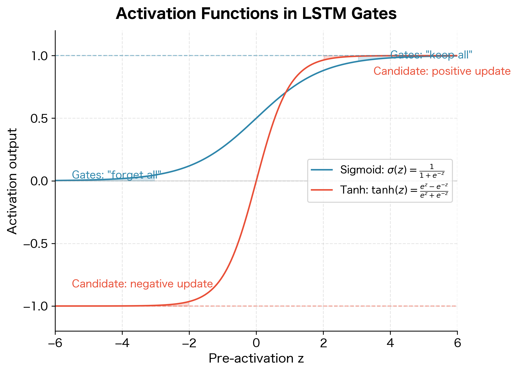
The sigmoid function is the mathematical heart of gating. It transforms any real number into a value between 0 and 1, perfect for representing "how much to keep":
where:
- : the input value (can be any real number)
- : the exponential function, which ensures the output is always positive
- The denominator normalizes the result to fall between 0 and 1
The sigmoid has a characteristic S-shape that makes it ideal for soft decisions. When the pre-activation is large and positive, approaches 0, so , meaning "keep this memory." When is large and negative, becomes very large, so , meaning "forget this." For intermediate values, the sigmoid produces intermediate retention levels, allowing the network to partially dim memories rather than making hard binary choices.
Understanding the Dimensions
Let's trace through the matrix dimensions carefully. Suppose we have an input dimension (e.g., 100-dimensional word embeddings) and hidden dimension .
The input transformation multiplies a matrix by a vector, producing a vector. The hidden state transformation multiplies a matrix by a vector, also producing a vector. These two vectors are added element-wise along with the bias, then sigmoid is applied element-wise to produce the final forget gate vector.
Initialization Matters
The forget gate bias is often initialized to a positive value (commonly 1 or 2) rather than zero. This ensures that early in training, the forget gate outputs values close to 1, meaning the network starts by remembering everything. Without this initialization trick, the network might learn to forget too aggressively before it has learned what information is worth keeping.
The Input Gate
While the forget gate decides what to discard, the input gate addresses the complementary question: what new information deserves to be written into memory? Not every input is equally important. When reading text, some words carry crucial meaning ("The murderer was...") while others are grammatical scaffolding ("the", "was"). The input gate learns to recognize which incoming information warrants permanent storage.
The input gate works in tandem with a candidate cell state (which we'll examine next). Think of it as a two-stage process: the candidate proposes "here's what we could store," and the input gate decides "here's how much of that proposal to actually write." This separation of concerns allows the network to generate rich candidate updates while maintaining fine-grained control over what actually enters long-term memory.
The Gating Mechanism
Like the forget gate, the input gate examines the current input and previous hidden state to make context-dependent decisions:
where:
- : the input gate activation vector, controlling write intensity per dimension
- : weight matrix that learns which input features signal "important, store this"
- : weight matrix that learns which processing contexts warrant new storage
- : bias vector setting the default write behavior
The structure is identical to the forget gate: a linear combination of the input and hidden state, followed by sigmoid. The difference lies entirely in the learned parameters. During training, the network discovers that certain input patterns should trigger forgetting while different patterns should trigger storage. The same architectural template serves opposite purposes through different learned weights.
The Candidate Cell State
The input gate decides how much to write, but something must decide what to write. This is the role of the candidate cell state: it proposes the actual content that might be added to memory. Think of it as drafting a memo that may or may not be filed, depending on the input gate's judgment.
The candidate needs to be expressive. It should be able to propose increases to certain memory dimensions, decreases to others, and leave some unchanged. This flexibility is crucial because the cell state encodes information through both the magnitude and sign of its values. A sentiment analysis model, for instance, might use positive cell state values to encode positive sentiment and negative values for negative sentiment. The candidate must be able to push the cell state in either direction.
The Candidate Formula
Like the gates, the candidate examines the current input and previous hidden state:
where:
- : the candidate cell state vector, proposing potential updates
- : weight matrix that learns what content to extract from the input
- : weight matrix that learns how recent processing should shape the update
- : bias vector
Why tanh Instead of Sigmoid?
Notice the crucial difference: the candidate uses instead of sigmoid. The hyperbolic tangent function is defined as:
where is the input value. This function outputs values in the range , centered around zero. The centering is key: unlike sigmoid, which only produces positive values between 0 and 1, can output negative values. This allows the candidate to propose both positive and negative updates to the cell state.
Consider what would happen if the candidate used sigmoid instead. The cell state could only ever increase (since you'd only be adding positive values). Information could accumulate but never be actively reversed. With , the candidate can propose "increase this dimension" (positive values) or "decrease this dimension" (negative values), giving the network the full expressiveness it needs.
The candidate cell state uses because it needs to propose values that can add to or subtract from the existing cell state. Sigmoid would only allow positive additions, severely limiting the network's representational power.
The Cell State Update
We've now assembled all the ingredients: a forget gate that knows what to discard, an input gate that knows how much to write, and a candidate that proposes what to write. The cell state update combines these three components into a single equation that forms the heart of the LSTM.
This is where the "information highway" metaphor becomes concrete. The cell state flows through time, modified at each step by two operations: selective forgetting and selective addition. The key insight is that information can flow unchanged for many time steps if the forget gate stays near 1 and the input gate stays near 0. This enables LSTMs to capture long-range dependencies.
The Update Equation
The new cell state is computed as:
where:
- : the new cell state
- : the previous cell state (the memory we're updating)
- : the forget gate activation (values between 0 and 1)
- : the input gate activation (values between 0 and 1)
- : the candidate cell state (values between -1 and 1)
- : the Hadamard (element-wise) product, where
Understanding the Two Terms
The equation has two terms, each serving a distinct purpose:
Term 1: Filtered Memory ()
This term takes the previous cell state and scales each dimension by the corresponding forget gate value. If for dimension , then 90% of that dimension's previous value is retained. If , only 10% survives. This element-wise multiplication allows the network to selectively preserve some memories while erasing others, all within the same time step.
Term 2: New Information ()
This term takes the candidate's proposal and scales it by the input gate. If for dimension , then 80% of the candidate's proposed value for that dimension gets written. If , the candidate's proposal is largely ignored. This gating prevents irrelevant information from contaminating the cell state.
The Sum: Combining Old and New
Adding these terms creates the new cell state. Each dimension independently combines its filtered old value with its gated new value. This additive structure is crucial for gradient flow: during backpropagation, gradients can flow directly through the addition operation without being squashed by nonlinearities.
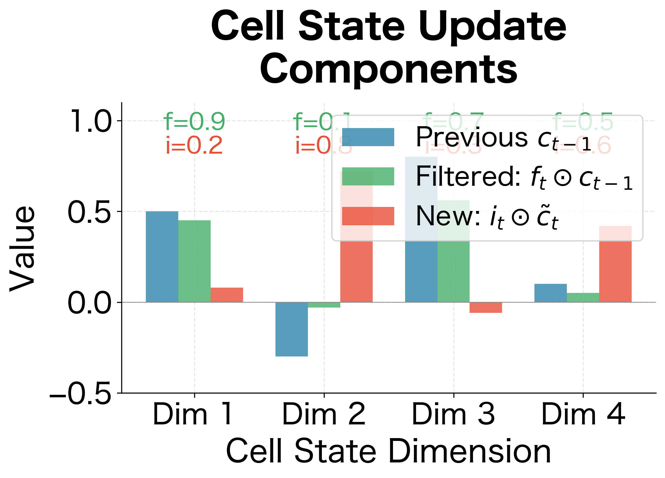
A Concrete Example: Tracing the Update Step by Step
Let's walk through a concrete example to see exactly how the gates interact. Suppose the cell state has dimension and at time we have:
- Previous cell state:
- Forget gate:
- Input gate:
- Candidate:
Step 1: Apply the forget gate to the previous cell state
Step 2: Apply the input gate to the candidate
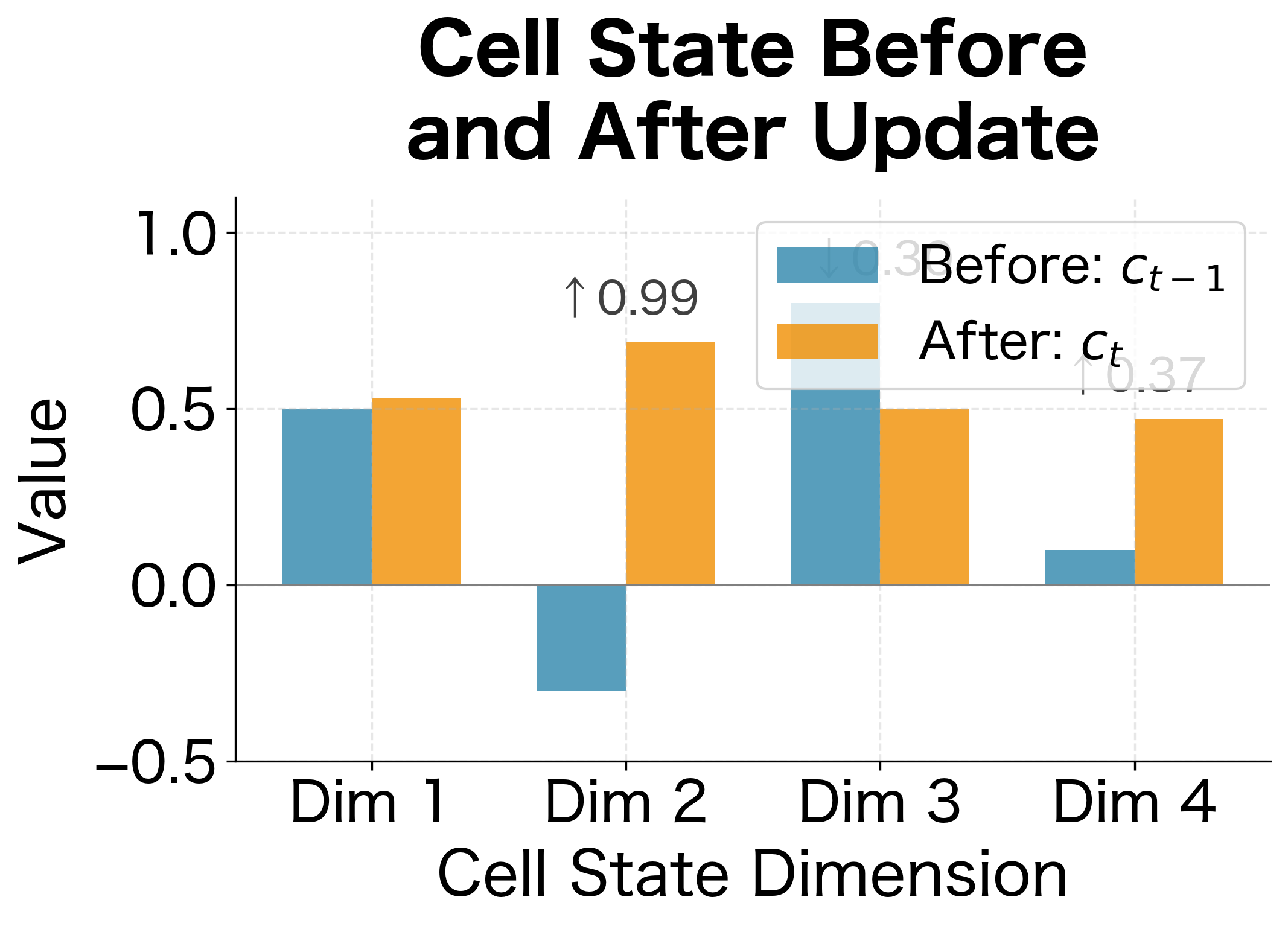
Step 3: Sum to get the new cell state
Interpreting Each Dimension:
-
Dimension 1 (): The forget gate was high (0.9), preserving most of the old value. The input gate was low (0.2), adding little new information. Result: minimal change, memory preserved.
-
Dimension 2 (): The forget gate was low (0.1), nearly erasing the old value. The input gate was high (0.8), strongly writing the candidate's positive value. Result: dramatic reversal, old memory replaced with new information.
-
Dimension 3 (): Moderate forget gate (0.7) kept most of the old value. Low input gate (0.3) added a small negative candidate contribution. Result: gradual decrease.
-
Dimension 4 (): Balanced gates (0.5 and 0.6) created a blend of old and new. Result: moderate change incorporating both sources.
This example illustrates the LSTM's power: each dimension of the cell state can be updated independently, with different balances of remembering and writing, all controlled by the learned gate values.
The Output Gate
The cell state now contains the LSTM's updated memory, but not all of this memory is relevant for the current moment. Consider a language model that has stored information about the subject of a sentence ("The cat"), the ongoing action ("is chasing"), and various contextual details. When predicting the next word, only some of this stored information is immediately relevant. The output gate acts as a filter, selecting which parts of the internal memory to expose for the current output.
This separation between internal memory (cell state) and external output (hidden state) is a key architectural insight. The cell state can accumulate and preserve information over long time spans, while the hidden state provides a task-relevant summary at each step. The output gate bridges these two representations.
The Output Gate Equation
Following the same pattern as the other gates, the output gate examines the current context:
where:
- : the output gate activation vector, controlling what to expose
- : weight matrix that learns which input features signal "this memory is now relevant"
- : weight matrix that learns which processing contexts warrant exposing certain memories
- : bias vector
The structure matches the other gates: linear combination followed by sigmoid. But the purpose is different. While the forget and input gates control what goes into memory, the output gate controls what comes out. This asymmetry allows the LSTM to store information that isn't immediately useful but may become relevant later.
The Hidden State Computation
The final step transforms the internal cell state into the external hidden state. This hidden state serves dual purposes: it becomes the LSTM's output for downstream processing (feeding into the next layer or making predictions), and it provides the recurrent context for the next time step.
The Hidden State Formula
The hidden state is computed by filtering the normalized cell state through the output gate:
where:
- : the new hidden state, the LSTM's output at this time step
- : the output gate activation (values between 0 and 1)
- : the cell state squashed to the range
Why Apply tanh to the Cell State?
Notice that we apply to the cell state before gating. This serves two important purposes:
1. Normalization: The cell state can accumulate values well outside through repeated additions. If the forget gate stays near 1 and the input gate keeps adding positive values, the cell state could grow to 10, 100, or larger. Applying compresses these potentially large values back into a bounded range, preventing the hidden state from exploding.
2. Consistency: The hidden state feeds into subsequent layers and provides recurrent context. Having it bounded in makes the network's behavior more predictable and stable. Downstream layers can rely on receiving inputs within a consistent range.
The cell state can accumulate values outside through repeated updates. Applying before the output gate ensures the hidden state remains bounded, improving numerical stability and gradient flow.
The Complete Picture
With the hidden state computed, we've completed one full LSTM step. The hidden state now flows in two directions:
- Forward to the next layer (or to the output): providing the LSTM's representation of the sequence up to time
- Recurrently to the next time step: serving as when processing
Meanwhile, the cell state flows only recurrently, carrying the LSTM's long-term memory forward without being directly exposed to downstream processing. This dual-track architecture, with the cell state as a protected memory channel and the hidden state as a filtered output, is what gives LSTMs their ability to capture long-range dependencies.
Complete LSTM Equations
Let's collect all the equations in one place for reference. Given inputs , , and , the LSTM computes:
These six equations fully specify the LSTM cell. Notice the symmetry: three gates (forget, input, output) all have the same structure, differing only in their learned parameters. The candidate has the same structure but uses instead of sigmoid. The cell state and hidden state updates are simple element-wise operations.
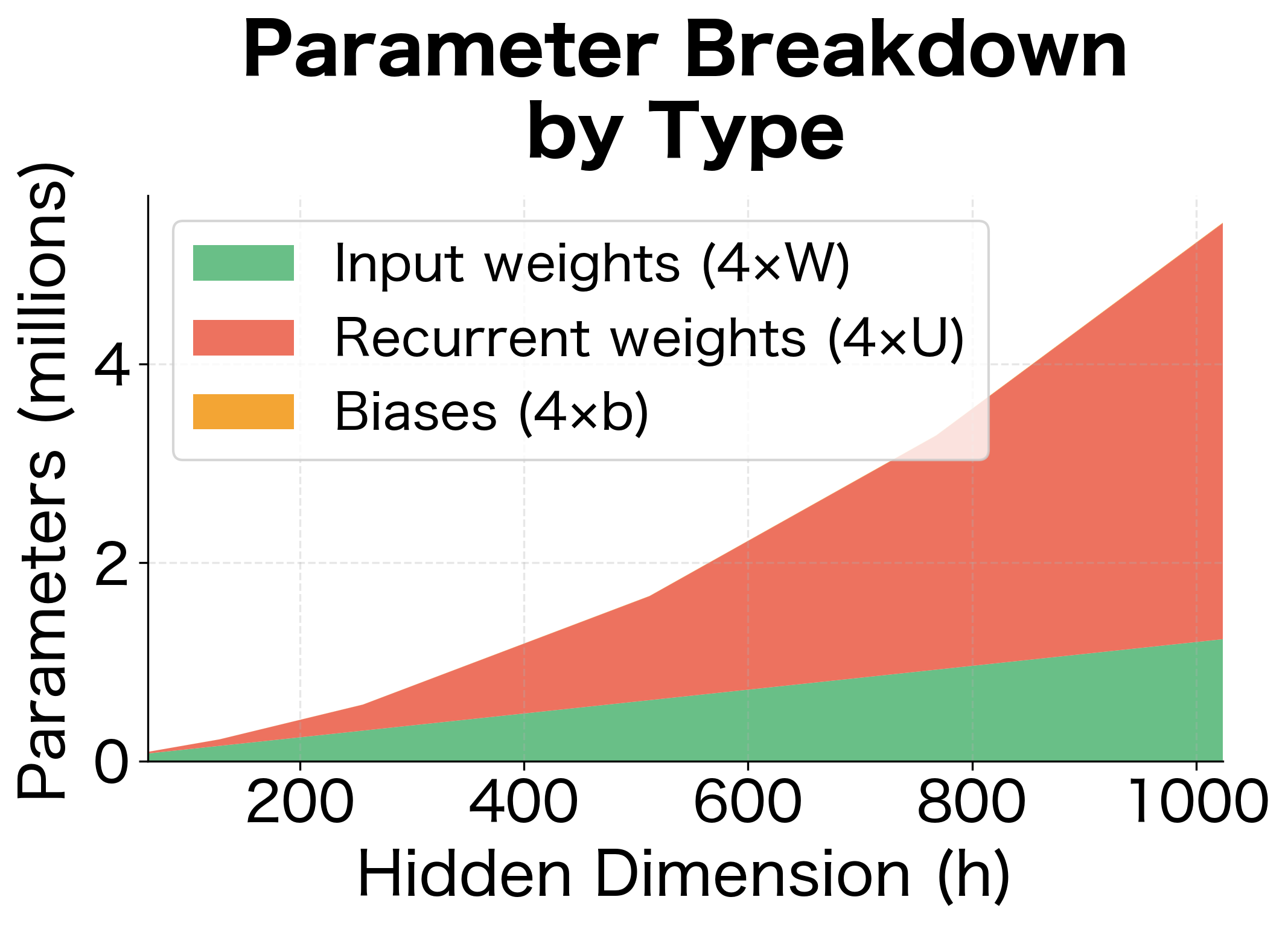
LSTM Parameter Count
Understanding the parameter count is essential for estimating memory requirements and comparing architectures. Let's count every learnable parameter in an LSTM cell.
Each gate (forget, input, output) and the candidate cell state has:
- One weight matrix for the input: parameters
- One weight matrix for the hidden state: parameters
- One bias vector : parameters
Since we have four such components (forget gate, input gate, candidate, output gate), the total parameter count is:
where:
- : the hidden dimension (size of the hidden and cell states)
- : the input dimension (size of the input vector at each time step)
- : parameters in each input weight matrix
- : parameters in each recurrent weight matrix
- : parameters in each bias vector
- The factor of 4 accounts for the four components (forget gate, input gate, candidate, output gate)
For a more compact form, we can factor this as:
where counts all weight matrix parameters and counts all bias parameters.
Example Calculation
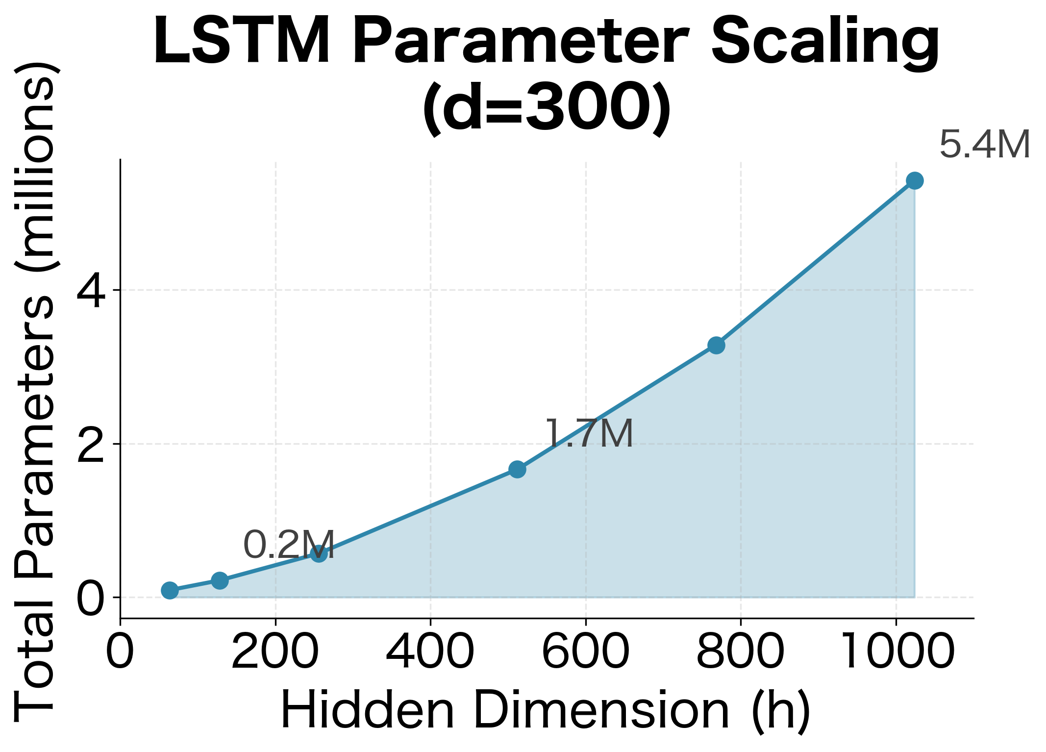
Let's compute the parameter count for a typical configuration with input dimension (common for word embeddings) and hidden dimension .
With these dimensions, a single LSTM layer has over 1.6 million parameters. For comparison, a vanilla RNN with the same dimensions would have:
where the single factor (instead of 4) reflects that a vanilla RNN has only one set of weights for its single transformation. The LSTM's four-fold increase in parameters comes from its four separate components (forget gate, input gate, candidate, output gate), each with their own weight matrices and biases.
Stacked LSTMs
When you stack multiple LSTM layers, the parameter count increases. The first layer takes the input dimension , but subsequent layers take the hidden dimension as their input (since they receive the previous layer's hidden state).
A 3-layer LSTM with these dimensions has over 5.7 million parameters. Deep language models often use even larger hidden dimensions and more layers, quickly reaching hundreds of millions of parameters.
Implementing LSTM from Scratch
Now let's implement an LSTM cell from scratch using only NumPy. This exercise solidifies understanding and reveals the computational structure hidden behind framework abstractions.
Activation Functions
First, we need the sigmoid and tanh activation functions:
The sigmoid implementation handles numerical stability by using different formulas for positive and negative inputs, avoiding overflow from large exponentials.
LSTM Cell Class
Now we implement the LSTM cell with explicit weight matrices for each component:
Let's verify our implementation produces outputs with the correct shapes:
The hidden state values are bounded between and because they're computed as the product of a sigmoid (range ) and a tanh (range ). The cell state values can exceed this range since they accumulate through addition.
Processing a Sequence
An LSTM processes sequences by applying the cell repeatedly, passing the hidden and cell states from one step to the next:
Let's process a sample sequence and examine how the hidden state evolves:
The LSTM produces a hidden state at each time step. For sequence classification, you typically use the final hidden state. For sequence-to-sequence tasks, you use all hidden states.
Visualizing Gate Activations
Let's visualize how the gates respond to a sequence, which reveals how the LSTM decides what to remember and forget:
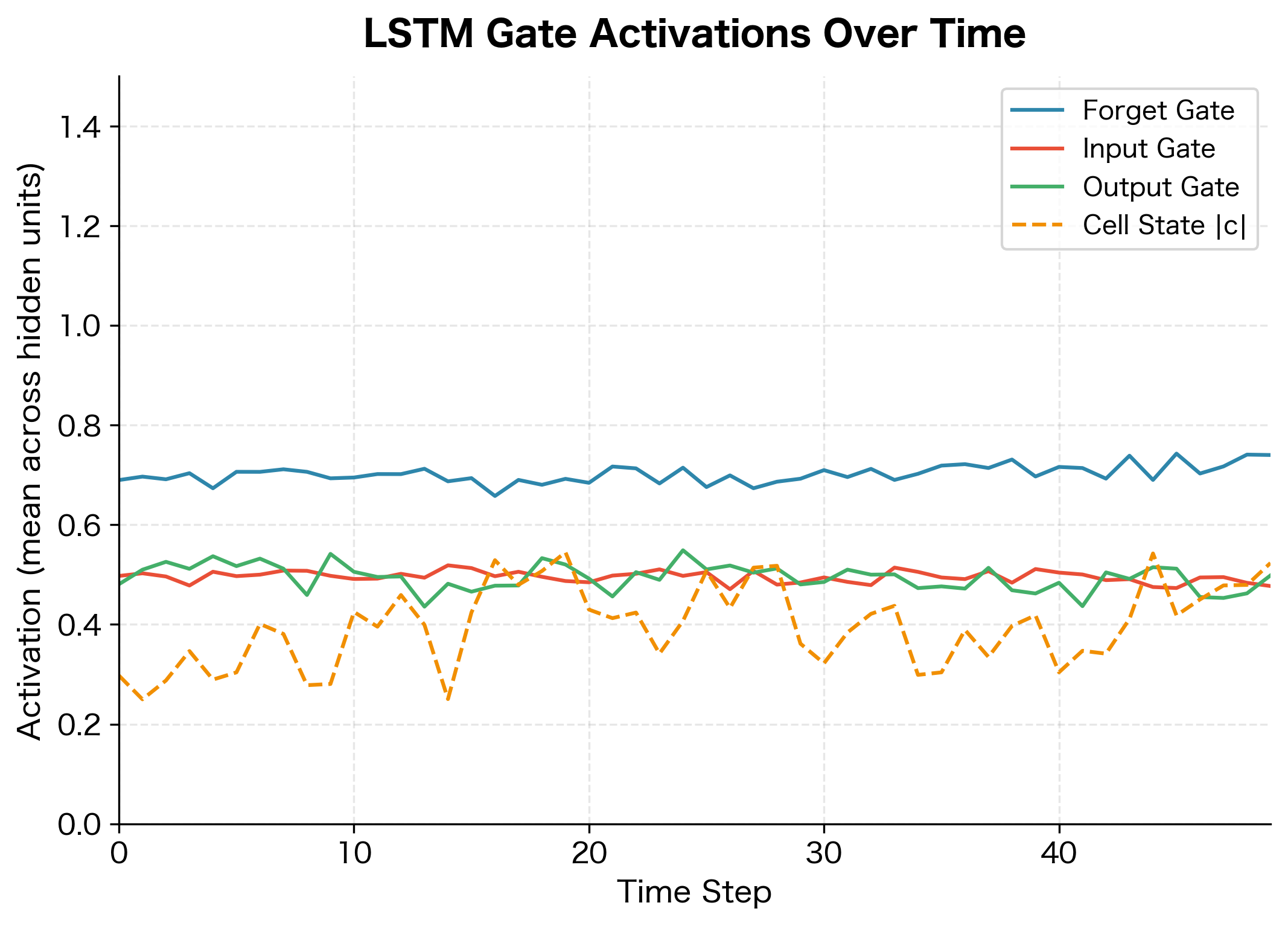
The visualization reveals several key behaviors. The forget gate starts high (near 1) because we initialized its bias to 1, causing the LSTM to preserve information by default. The input and output gates show more variation as they learn to selectively write and read. The cell state magnitude tends to grow over time as information accumulates, though the gates prevent unbounded growth.
Comparing with PyTorch
Let's verify our implementation matches PyTorch's LSTM by comparing outputs:
The outputs match to numerical precision, confirming our implementation is correct. The small differences (on the order of ) come from floating-point arithmetic variations between NumPy and PyTorch.
The Combined Weight Matrix Formulation
In practice, frameworks like PyTorch don't compute each gate separately. Instead, they concatenate all weight matrices and compute all gates in a single matrix multiplication, which is more efficient on GPUs.
The combined formulation stacks the four weight matrices vertically into single large matrices:
where:
- : combined input weight matrix, stacking all four gate input weights
- : combined recurrent weight matrix, stacking all four gate hidden weights
- : combined bias vector, concatenating all four gate biases
- The subscripts , , , denote input gate, forget gate, candidate, and output gate respectively
Then all gates are computed in one step:
The notation indicates that different activation functions are applied to different portions of the result: sigmoid to the first elements (input gate), sigmoid to the next elements (forget gate), tanh to the next elements (candidate), and sigmoid to the final elements (output gate).
This produces a -dimensional vector that is split into four chunks of size each. The efficiency gain comes from performing two large matrix multiplications instead of eight smaller ones.
Let's compare the performance of both implementations:
The efficient implementation is faster because it performs fewer matrix multiplications. The standard implementation does 8 matrix multiplications (2 per gate), while the efficient version does only 2 (one for inputs, one for hidden states). On GPUs, this difference is even more pronounced because large matrix multiplications are highly optimized.
Limitations and Practical Considerations
LSTMs represented a major breakthrough in sequence modeling, but they come with important limitations that practitioners should understand.
Computational Cost: Each time step requires sequential computation because the hidden state at time depends on the hidden state at time . This sequential dependency prevents parallelization across time steps, making LSTMs slow to train on long sequences. A 1000-step sequence requires 1000 sequential operations, regardless of how many GPUs you have. This is the fundamental limitation that motivated the development of Transformers, which can process all positions in parallel.
Memory Requirements: LSTMs must store hidden and cell states for every time step during training to enable backpropagation through time. For a sequence of length with hidden dimension , this requires memory per layer, where is the number of time steps and is the hidden state size. With long sequences and deep networks, memory can become a bottleneck. Techniques like truncated backpropagation through time can help, but they sacrifice gradient accuracy for long-range dependencies.
Gradient Flow: Despite the cell state's "information highway," gradients still face challenges over very long sequences. The forget gate must maintain values very close to 1 for hundreds of time steps to preserve gradients, which is difficult to learn. In practice, LSTMs struggle with dependencies beyond a few hundred time steps.
Hyperparameter Sensitivity: The hidden dimension, number of layers, learning rate, and gradient clipping threshold all interact in complex ways. LSTMs can be finicky to train, often requiring careful tuning. The forget gate bias initialization (setting it to 1 or 2) is one example of a trick that significantly affects training stability.
Despite these limitations, LSTMs remain valuable in many contexts. They are well-suited for streaming applications where you process data one element at a time. They work well for moderate-length sequences (up to a few hundred tokens). They also require less data to train than Transformers for smaller-scale problems. Understanding their equations deeply, as we've done in this chapter, helps you recognize when they're the right tool and when to reach for alternatives.
Key Parameters
When implementing or using LSTMs, several parameters significantly impact model behavior and performance:
-
hidden_dim (
hidden_sizein PyTorch): The dimensionality of the hidden and cell states. Larger values increase model capacity but also increase computation and memory. Common values range from 128 to 1024, with 256-512 being typical for many NLP tasks. -
input_dim (
input_sizein PyTorch): The dimensionality of the input vectors at each time step. This is typically determined by your embedding layer or feature representation. -
num_layers: The number of stacked LSTM layers. Deeper networks can learn more complex patterns but are harder to train. Most applications use 1-3 layers; beyond 4-5 layers, gradient flow becomes problematic without techniques like residual connections.
-
dropout: Regularization applied between LSTM layers (not within a single layer). Values of 0.2-0.5 are common. Note that dropout is only applied during training and when
num_layers > 1. -
bidirectional: Whether to process sequences in both directions. Bidirectional LSTMs double the effective hidden size but cannot be used for autoregressive generation tasks.
-
forget_bias (initialization): The initial value for the forget gate bias. Setting this to 1.0 or higher helps the network learn to preserve information early in training. This is often set implicitly by the framework but can be overridden.
-
batch_first: In PyTorch, determines whether input tensors have shape
(batch, seq, features)or(seq, batch, features). The former is more intuitive but the latter is the default for historical reasons.
Summary
This chapter translated the intuition of LSTM gates into precise mathematics and working code. The key equations form a system where three gates control information flow through a memory cell.
The Gate Equations:
- Forget gate: decides what to discard from memory
- Input gate: decides how much new information to write
- Candidate: proposes new values to store
- Output gate: decides what to expose as output
The State Updates:
- Cell state: combines filtered memory with gated new information
- Hidden state: exposes filtered cell state as output
Parameter Count:
An LSTM cell has parameters, where is the input dimension (e.g., word embedding size), is the hidden dimension, and the factor of 4 accounts for the four components (forget gate, input gate, candidate, output gate). This is four times the parameters of a vanilla RNN, reflecting the four separate learnable transformations.
Implementation Insights:
- Initializing the forget gate bias to 1 improves training by starting with full memory retention
- Combining weight matrices into single operations improves computational efficiency
- The cell state can grow unbounded, so applying tanh before the output gate maintains numerical stability
With these equations internalized, you can now trace exactly how information flows through an LSTM, debug unexpected behaviors, and make informed decisions about when to use this architecture. The next chapter examines how these equations enable better gradient flow compared to vanilla RNNs.
Quiz
Ready to test your understanding? Take this quick quiz to reinforce what you've learned about LSTM gate equations.

Comments