

Master Gated Recurrent Units (GRUs), the efficient alternative to LSTMs. Learn reset and update gates, implement from scratch, and understand when to choose GRU vs LSTM.

This article is part of the free-to-read Language AI Handbook
Choose your expertise level to adjust how many terms are explained. Beginners see more tooltips, experts see fewer to maintain reading flow. Hover over underlined terms for instant definitions.
GRU Architecture
In the previous chapters, we explored how LSTMs solve the vanishing gradient problem through their cell state and gating mechanisms. LSTMs work remarkably well, but their complexity comes at a cost: four separate weight matrices, two state vectors, and a substantial parameter count. In 2014, Cho et al. asked a natural question: can we achieve similar performance with a simpler architecture?
The Gated Recurrent Unit (GRU) is their answer. GRUs retain the core insight of LSTMs, using gates to control information flow, but streamline the design by merging the cell state and hidden state into a single vector and reducing three gates to two. This simplification often achieves comparable performance to LSTMs while training faster and using fewer parameters. Understanding when and why to choose GRUs over LSTMs is an essential skill for any sequence modeling practitioner.
GRU vs LSTM: The Key Differences
Before diving into the mechanics, let's establish what makes GRUs different from LSTMs. The comparison illuminates the design philosophy behind both architectures.
The key structural differences are:
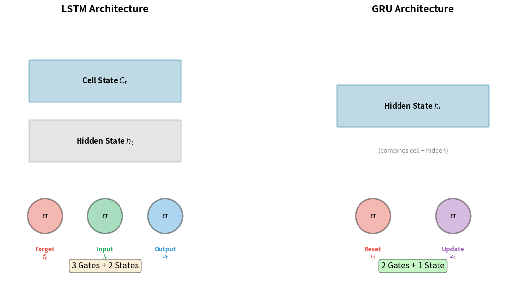
- State vectors: LSTMs maintain two state vectors (cell state and hidden state ), while GRUs use only one (hidden state ). The GRU's hidden state plays both roles.
- Number of gates: LSTMs have three gates (forget, input, output), while GRUs have two (reset, update). The update gate combines the forget and input gate functions.
- Parameter count: With fewer gates and one less state vector, GRUs have roughly 25% fewer parameters than LSTMs of equivalent hidden size.
Despite these simplifications, GRUs retain the essential capability that makes gated architectures powerful: the ability to selectively remember and forget information over long sequences. The question is whether the simplification sacrifices important expressiveness.
The Reset Gate: Controlling Past Influence
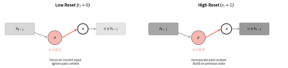
The reset gate determines how much of the previous hidden state should influence the computation of the new candidate hidden state. Think of it as asking: "How relevant is what I was thinking about to what I'm seeing now?"
When the reset gate outputs values close to 0, the GRU essentially ignores the previous hidden state and computes a new candidate based primarily on the current input. When it outputs values close to 1, the previous hidden state fully participates in computing the candidate. This mechanism allows the GRU to learn when to start fresh versus when to build on past context.
The reset gate computation follows the familiar gating pattern. It takes the previous hidden state and current input, concatenates them, applies a linear transformation, and passes the result through a sigmoid activation:
where:
- : the reset gate output, a vector of dimension with values in
- : the reset gate's weight matrix of shape , where is the input dimension and is the hidden dimension
- : concatenation of previous hidden state and current input, producing a vector of dimension
- : the reset gate's bias vector of dimension
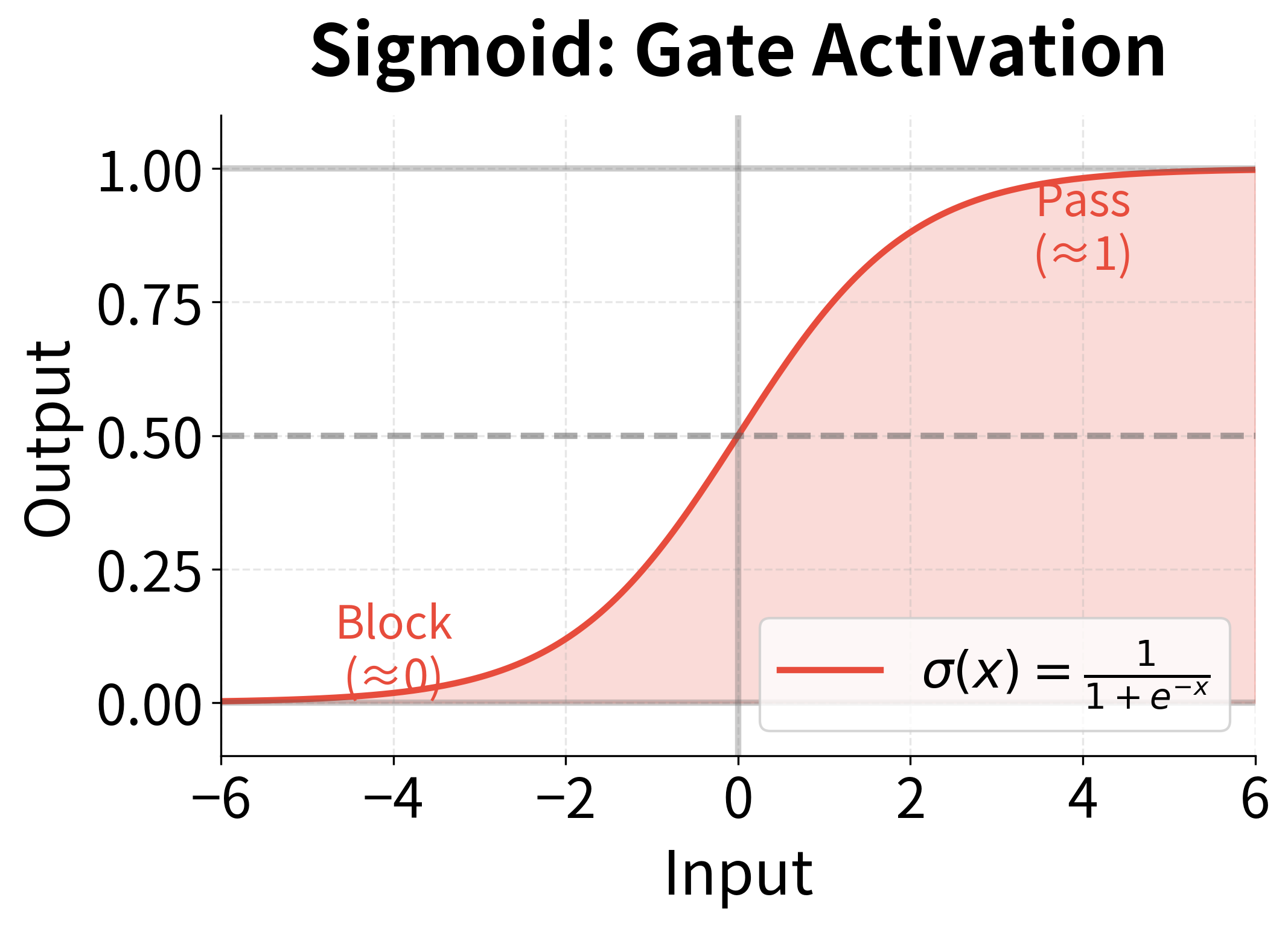
- : the sigmoid activation function, which squashes any real value to the range
The sigmoid activation is crucial here: it ensures every element of lies between 0 and 1, making it suitable for element-wise multiplication as a "soft switch." Values near 0 effectively block information, while values near 1 allow information to pass through unchanged.
The reset gate examines both what the model was thinking about () and what it's currently seeing () to decide how to weight past information. In language modeling, for instance, the reset gate might learn to output values near 0 when encountering a period or paragraph break, signaling that the previous context is no longer relevant and the model should begin fresh.
The Update Gate: Balancing Old and New
The update gate is the GRU's most distinctive feature. It performs double duty, simultaneously deciding how much of the old hidden state to retain and how much of the new candidate to incorporate. This elegant mechanism replaces the separate forget and input gates of the LSTM.
The update gate computation mirrors the reset gate's structure, using its own learned weights:
where:
- : the update gate output, a vector of dimension with values in
- : the update gate's weight matrix of shape
- : concatenation of previous hidden state and current input
- : the update gate's bias vector of dimension
- : the sigmoid activation function
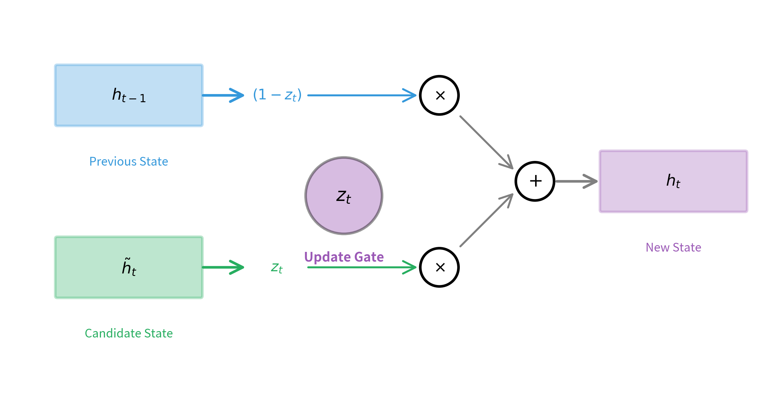
The key insight is how is used in the final state update. Rather than simply replacing the old state with the new candidate, the GRU computes a weighted average:
where:
- : the new hidden state at timestep
- : the previous hidden state from timestep
- : the candidate hidden state (computed using the reset gate)
- : the update gate output, controlling the interpolation
- : element-wise (Hadamard) multiplication
- : the complement of the update gate, representing "how much to keep"
This formula creates a smooth interpolation between the old state and the new candidate. Consider what happens at the extremes:
- When : the formula becomes . The hidden state is copied directly from the previous timestep with no modification, creating a perfect information highway.
- When : the formula becomes . The hidden state is completely replaced by the new candidate.
- When : the formula becomes . The new state is 70% old information and 30% new.
This weighted average is computed element-wise, so different dimensions of the hidden state can have different update rates. Some dimensions might preserve information across many timesteps while others update frequently.
In LSTMs, the forget gate and input gate operate independently. You could theoretically forget everything while adding nothing, or add new information without forgetting anything. The GRU's update gate enforces a constraint: the amount you forget and the amount you add must sum to 1. This constraint reduces flexibility but also reduces the parameter count and can act as a regularizer.
The Candidate Hidden State
Before the update gate can blend old and new information, we need to compute what the "new" information actually is. The candidate hidden state represents what the hidden state would become if we completely ignored the update gate's blending.
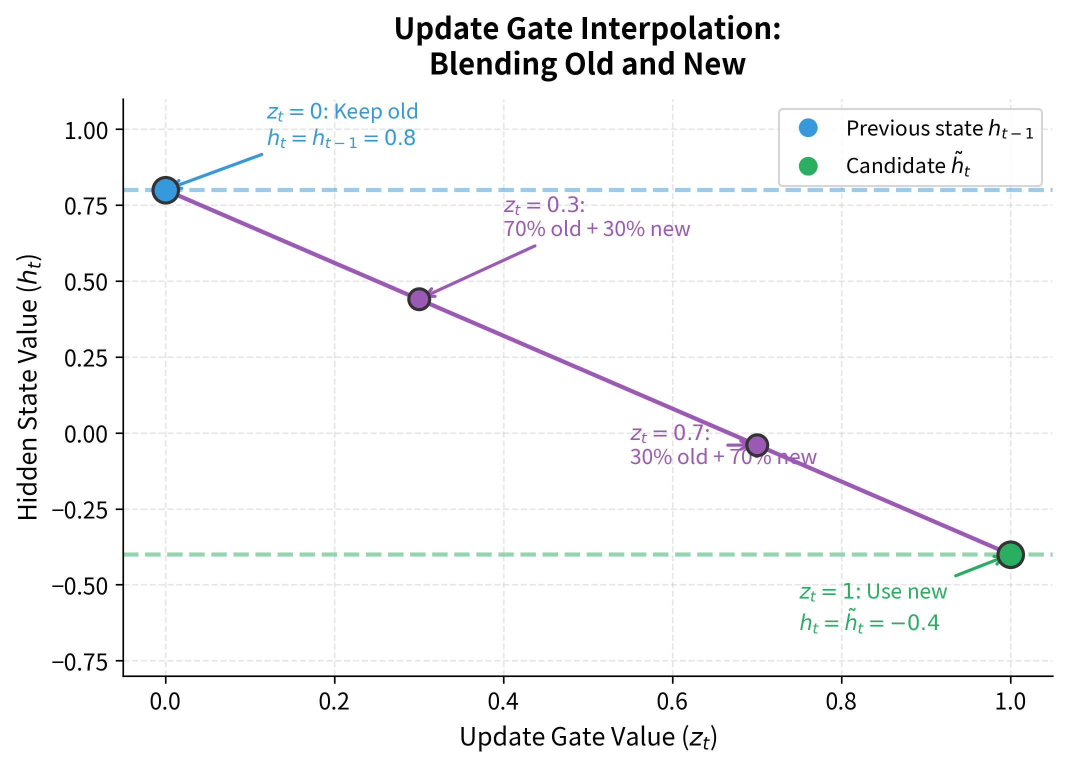
This is where the reset gate comes into play. The candidate computation uses the reset-gated version of the previous hidden state, not the raw hidden state:
where:
- : the candidate hidden state, a vector of dimension with values in
- : the reset gate output from the previous computation
- : the reset-gated previous hidden state, where denotes element-wise multiplication
- : concatenation of the reset-gated hidden state and current input
- : the candidate's weight matrix of shape
- : the candidate's bias vector of dimension
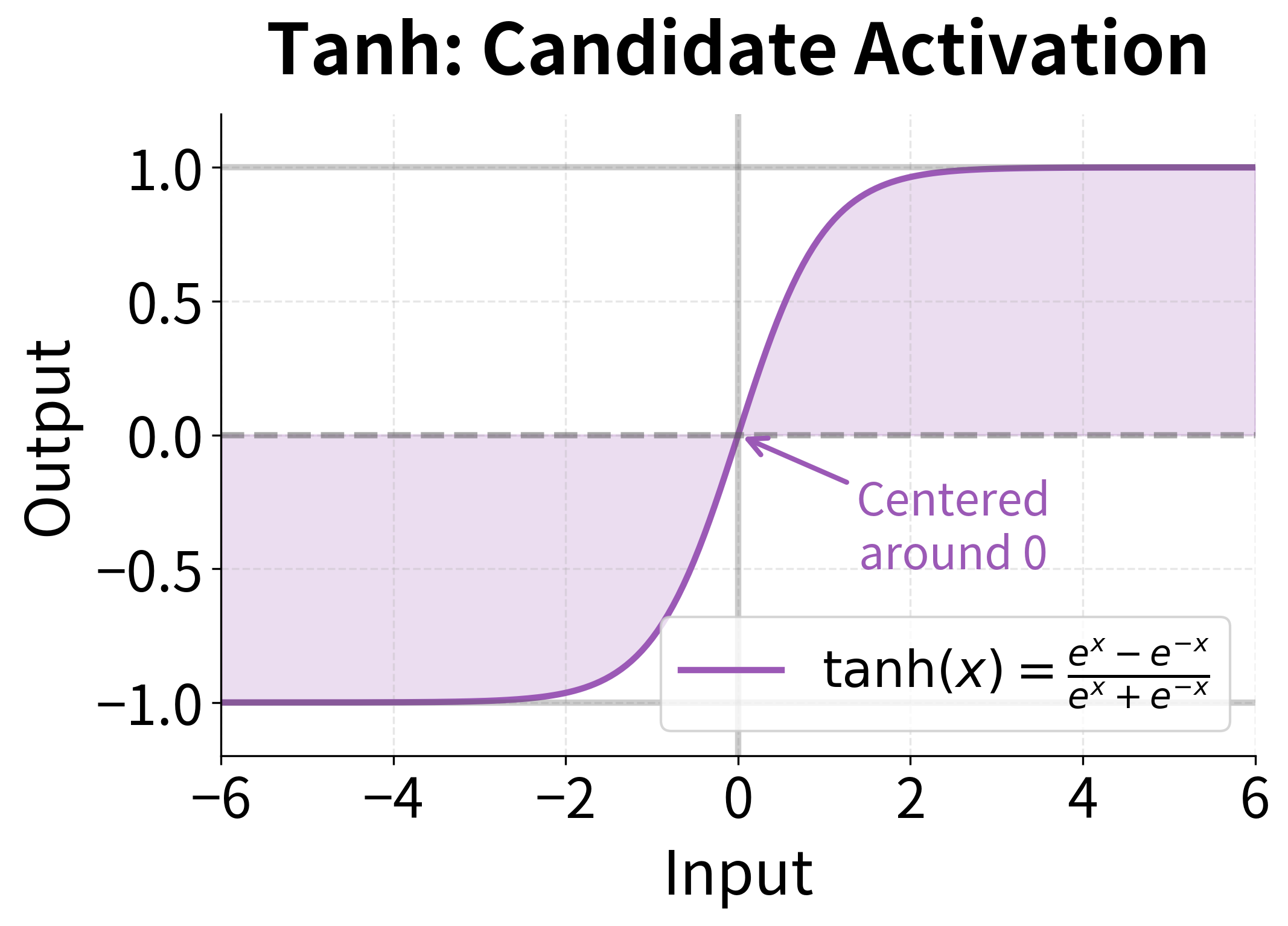
- : hyperbolic tangent activation function, outputting values in
The tanh activation serves two important purposes. First, it bounds the candidate values to a reasonable range , preventing any single dimension from growing unboundedly. Second, it centers the values around zero, which helps with gradient flow during training and allows the hidden state to both increase and decrease in value.
The reset gate's role is clearer now. By gating before it enters the candidate computation, the reset gate controls how much the previous context influences the new candidate:
- When : the term , so the candidate depends primarily on the current input
- When : the term , so the candidate incorporates the full previous context
This gives the GRU two distinct ways to control information flow: the reset gate decides how much past context influences the proposal for the new state, while the update gate decides how much of that proposal to actually accept.
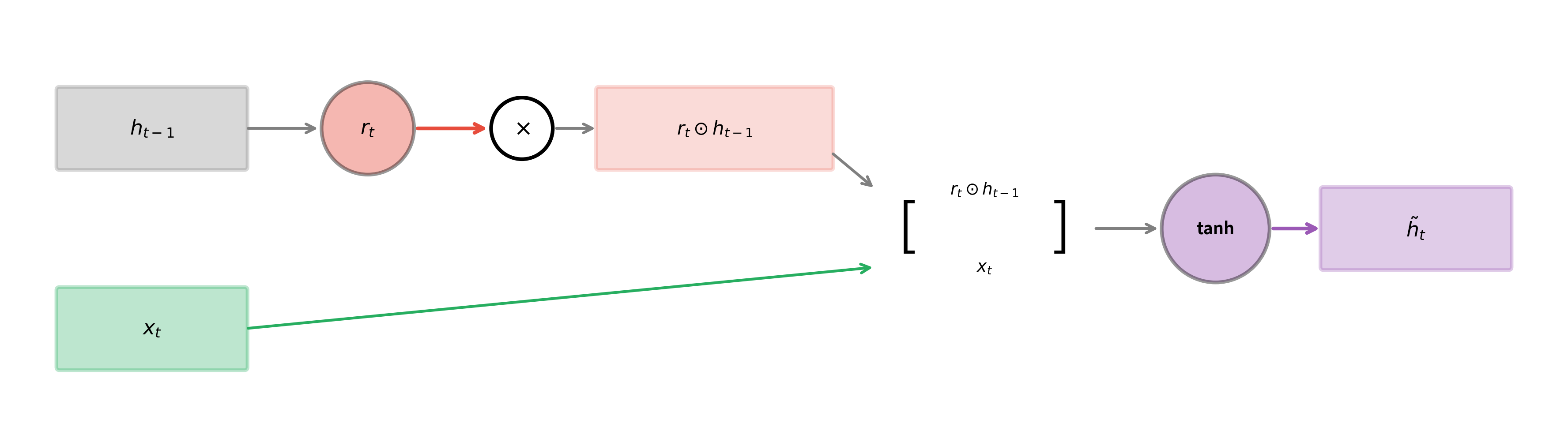
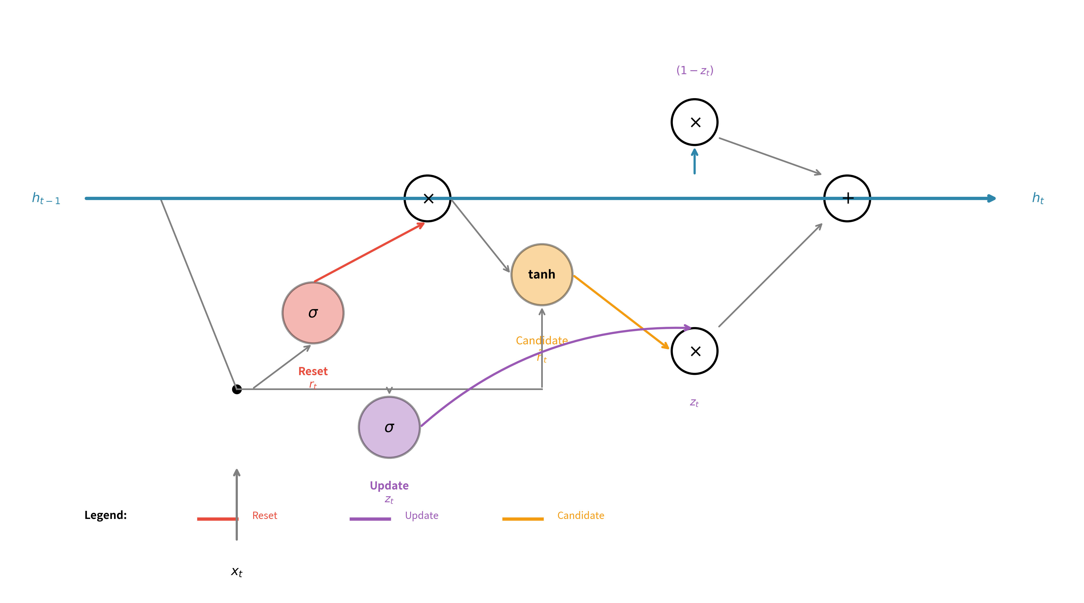
Complete GRU Equations
Having explored each component individually, we're now ready to see how they fit together into a unified computational framework. The beauty of the GRU lies not in any single equation, but in how these pieces orchestrate a delicate dance of remembering and forgetting at every timestep.
Imagine you're reading a novel. At each word, your brain performs a remarkable feat: it decides which aspects of the previous context remain relevant, proposes an updated understanding, and then blends this new understanding with what you already knew. The GRU mirrors this process through four sequential computations, each building on the previous.
The Four-Step Computation
At each timestep , the GRU receives two inputs: the previous hidden state (what the model "remembers" from processing earlier timesteps) and the current input (the new information arriving now). From these, it must produce a new hidden state that appropriately blends old context with new observations.
Step 1: Assess how much to update (the update gate)
Before doing anything else, the GRU asks: "Given what I knew and what I'm seeing now, how much should I change my understanding?" The update gate answers this question:
This gate examines both the previous hidden state and current input, then outputs a value between 0 and 1 for each dimension of the hidden state. A value near 0 means "keep the old information," while a value near 1 means "embrace the new." The sigmoid function ensures these values stay in the valid range.
Step 2: Determine past relevance (the reset gate)
Next, the GRU considers a subtler question: "When computing my proposal for new information, how much should the past influence that proposal?" The reset gate provides this answer:
This gate has a different purpose than the update gate. While the update gate controls the final blending, the reset gate controls what goes into the "new" option being considered. When the reset gate outputs values near 0, the GRU effectively ignores its memory when formulating a new candidate, allowing it to make a fresh start.
Step 3: Propose new content (the candidate hidden state)
With the reset gate computed, the GRU can now propose what the new hidden state might look like. This candidate incorporates the current input and a reset-modulated version of the previous state:
The notation represents element-wise multiplication: each dimension of is scaled by the corresponding dimension of . Where the reset gate is low, the previous hidden state's influence is suppressed; where it's high, the previous state participates fully. The tanh activation bounds the candidate to , preventing unbounded growth.
Step 4: Blend old and new (the final hidden state)
Finally, the GRU combines everything using the update gate as a blending coefficient:
This formula is a weighted average computed element-wise. For each dimension of the hidden state:
- The term represents how much of the old value to keep
- The term represents how much of the new candidate to add
- Since , the weights always sum to one
This constraint is what distinguishes GRUs from LSTMs: you cannot simultaneously keep everything old and add everything new. The architecture forces a trade-off, which reduces flexibility but also reduces parameters and can act as implicit regularization.
Understanding the Notation
Throughout these equations, we use consistent notation:
- : previous hidden state, a vector of dimension
- : current input, a vector of dimension
- : concatenation of the two vectors, producing a vector of dimension
- : learnable weight matrices, each of shape
- : learnable bias vectors, each of dimension
- : the sigmoid function, , outputs in
- : the hyperbolic tangent function, outputs in
- : element-wise (Hadamard) multiplication
The Interplay of Gates
The elegance of the GRU emerges from how these equations interact. Consider two extreme scenarios:
Scenario 1: Encountering a sentence boundary. When the model sees a period followed by a capital letter, it might learn to set the reset gate low (near 0) and the update gate high (near 1). The low reset gate means the candidate is computed almost entirely from the new input, ignoring the previous sentence's context. The high update gate then replaces most of the old hidden state with this fresh candidate. Result: the model "forgets" the previous sentence and starts fresh.
Scenario 2: Processing a long noun phrase. When the model is in the middle of "the large, spotted, energetic dog," it might learn to keep the reset gate high (preserving context about "the large, spotted") while setting the update gate to moderate values (blending new adjectives with existing understanding). Result: the model accumulates information about the noun phrase without losing track of what came before.
The network learns these patterns automatically through backpropagation, adjusting the weight matrices , , and to produce appropriate gate values for each situation it encounters during training.
GRU Parameter Efficiency
One of the GRU's main selling points is its reduced parameter count compared to LSTMs. Let's quantify this difference precisely.
For a single-layer recurrent network with input size and hidden size , each gate or transformation requires:
- A weight matrix of shape , contributing parameters
- A bias vector of shape , contributing parameters
- Total per gate: parameters
LSTM parameters (4 gates/transformations):
- Forget gate: parameters
- Input gate: parameters
- Cell candidate: parameters
- Output gate: parameters
- Total:
GRU parameters (3 gates/transformations):
- Reset gate: parameters
- Update gate: parameters
- Candidate: parameters
- Total:
The ratio of GRU to LSTM parameters is:
The GRU has exactly 75% of the LSTM's parameters, regardless of the input and hidden dimensions. For typical configurations, this translates to meaningful savings in memory, training time, and inference speed.
The ratio remains exactly 75% regardless of the input or hidden dimensions, confirming our mathematical derivation. As models scale up, the absolute parameter savings become substantial: for a large model with hidden size 1024, the GRU saves over 3 million parameters compared to an equivalent LSTM. These savings translate directly to reduced memory usage during training and inference, faster gradient computations, and potentially better generalization on smaller datasets.
The 25% parameter reduction has several practical implications. Training is faster because there are fewer gradients to compute and fewer weights to update. Memory usage is lower, allowing larger batch sizes or longer sequences. And with fewer parameters, GRUs may be less prone to overfitting on smaller datasets.
The following table shows parameter counts for various hidden sizes with a fixed input size of 256:
| Hidden Size | LSTM Parameters | GRU Parameters | GRU/LSTM Ratio |
|---|---|---|---|
| 128 | 394,752 | 296,064 | 75% |
| 256 | 1,050,624 | 787,968 | 75% |
| 512 | 3,149,824 | 2,362,368 | 75% |
| 768 | 6,300,672 | 4,725,504 | 75% |
| 1024 | 10,489,856 | 7,867,392 | 75% |
Implementing a GRU from Scratch
Theory becomes concrete through implementation. By building a GRU cell from scratch using only NumPy, we'll see exactly how the mathematical equations translate into executable code. This exercise reveals the simplicity underlying the architecture: despite the sophisticated behavior GRUs can learn, the forward pass is just a sequence of matrix multiplications, element-wise operations, and activation functions.
Setting Up the Activation Functions
Before implementing the GRU itself, we need the two activation functions that appear in the equations. The sigmoid function maps any real number to the interval , making it perfect for gates. The tanh function maps to , centering values around zero for the candidate computation.
The sigmoid implementation uses a numerically stable form that avoids overflow for large negative inputs. For , we compute directly. For , we use the equivalent form , which avoids computing for large negative .
The GRU Cell Class
Now we can implement the GRU cell. The class needs to store three sets of parameters (one for each gate/transformation) and implement the forward pass that computes the four steps we discussed.
Let's trace through the key parts of this implementation:
-
Weight initialization: We use Xavier initialization, scaling weights by where is the input dimension and is the hidden dimension. This keeps the variance of activations roughly constant across layers, which helps with training stability.
-
Concatenation: The line
concat = np.vstack([h_prev, x])creates the vector that both gates receive as input. By stacking vertically, we create a single vector of dimension . -
Gate computations: Each gate follows the same pattern: matrix multiply, add bias, apply sigmoid. The
@operator performs matrix multiplication in NumPy. -
Reset-gated candidate: The candidate computation is slightly more complex because it uses the reset-gated hidden state. We first compute
reset_hidden = r * h_prev(element-wise multiplication), then concatenate this with the input before the matrix multiplication. -
Final blending: The last line implements the weighted average formula, using NumPy's broadcasting for element-wise operations.
Testing the Implementation
Let's verify our implementation by processing a short sequence and examining how the gates behave. With randomly initialized weights, we expect the gates to output values near 0.5 (since sigmoid of values near zero is approximately 0.5).
The results confirm our expectations. With randomly initialized weights, the gate activations hover around 0.5, reflecting the sigmoid function's output for inputs near zero. The reset gate mean of approximately 0.5 indicates that the network is partially incorporating past context into the candidate computation. Similarly, the update gate mean near 0.5 means the hidden state update is roughly half old information and half new candidate.
Notice how the hidden state L2 norm grows modestly across timesteps. Starting from zero, the hidden state accumulates information as each timestep contributes new content. The growth is bounded because tanh keeps the candidate values in , and the update gate's blending prevents explosive growth.
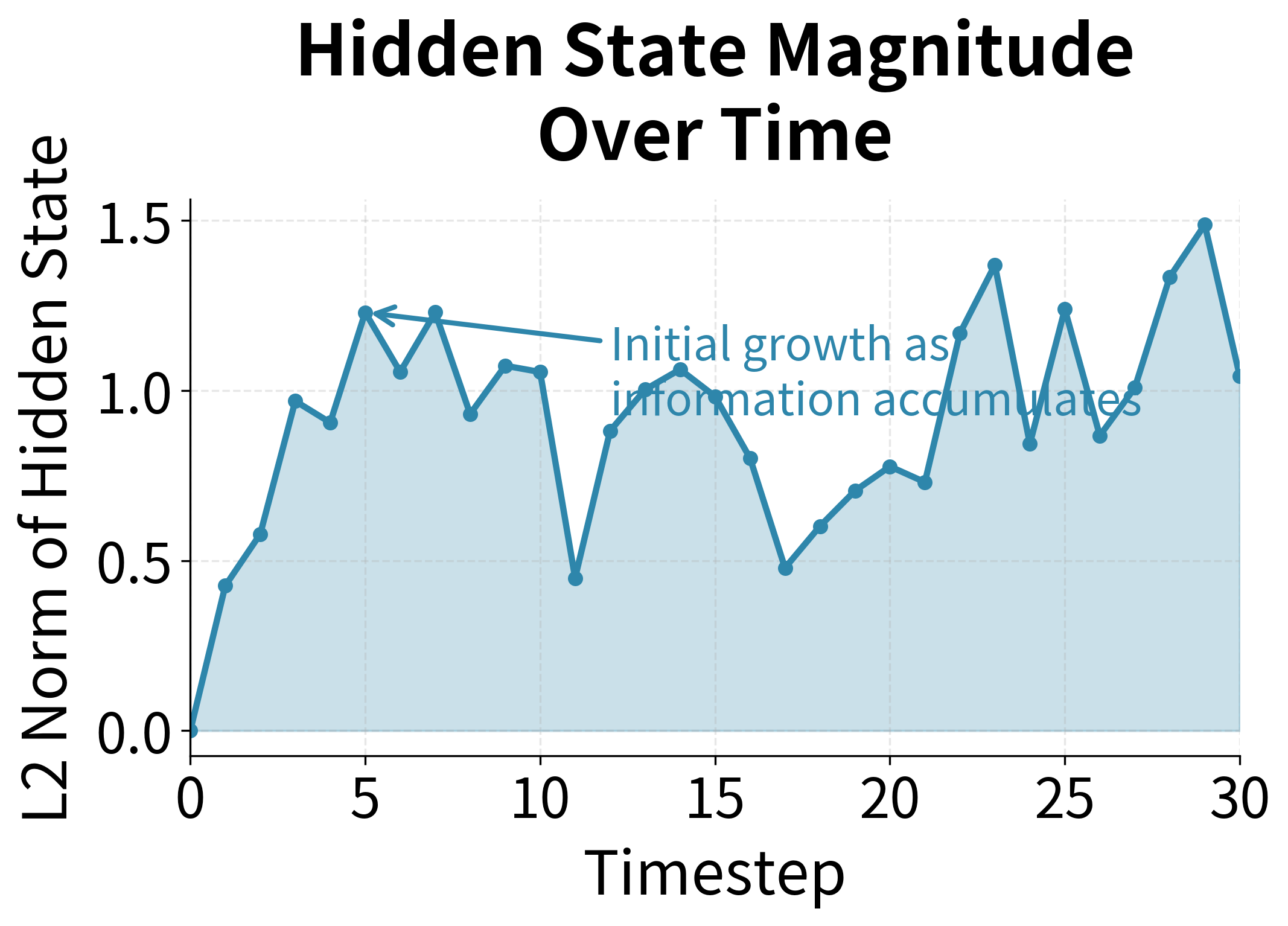
The left panel shows that the hidden state's magnitude (L2 norm) grows initially as information from the input sequence accumulates, then tends to stabilize. This bounded growth is a direct consequence of the tanh activation, which constrains candidate values to , and the update gate's weighted averaging, which prevents any single timestep from causing explosive changes.
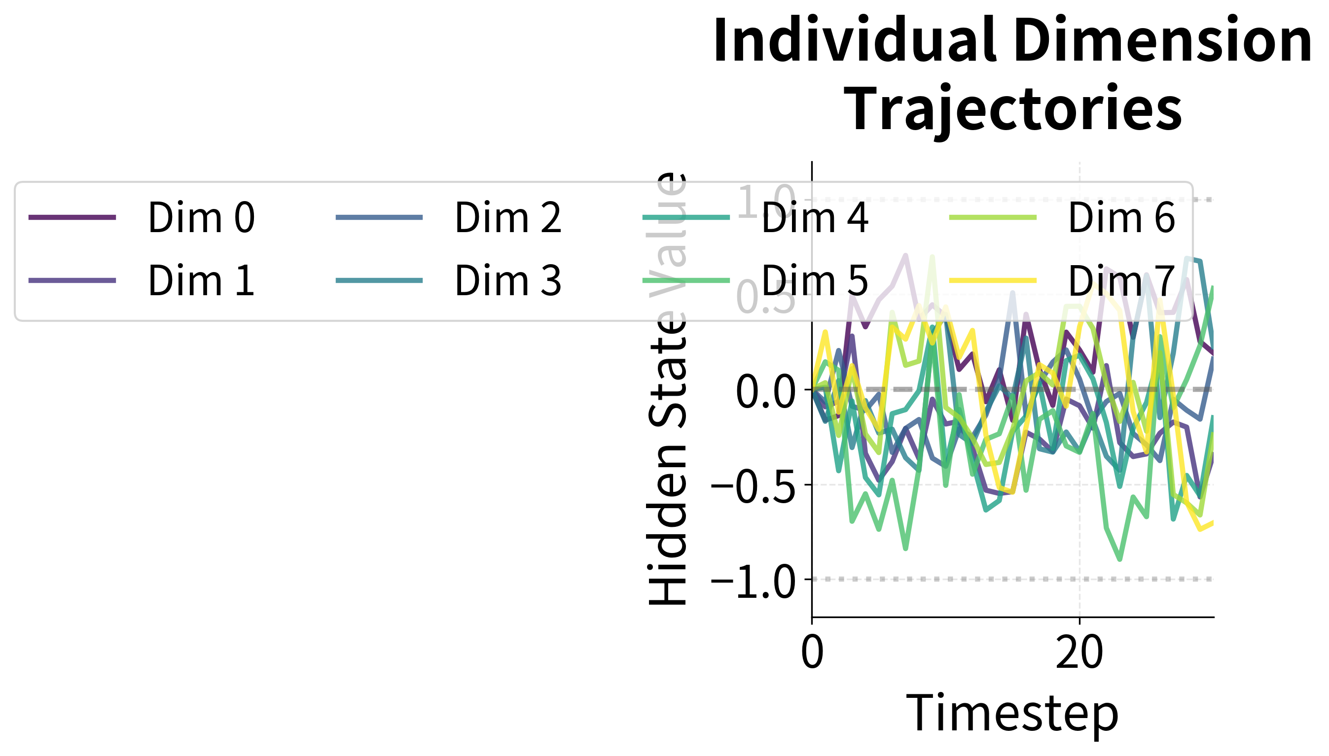
The right panel reveals that different dimensions of the hidden state follow diverse trajectories. Some dimensions oscillate around zero, others trend positive or negative, and some remain relatively stable. This diversity is essential: it allows the GRU to track multiple aspects of the input sequence simultaneously. After training, these dimensions would specialize to capture different semantic features relevant to the task.
After training on actual data, these gate activations would show more pronounced patterns. Instead of hovering near 0.5, they would swing closer to 0 or 1 depending on the learned task requirements. A language model, for instance, might learn to push the reset gate toward 0 at sentence boundaries and toward 1 within sentences.
Let's visualize how the gates and hidden state evolve across a longer sequence to see the full picture of GRU dynamics.
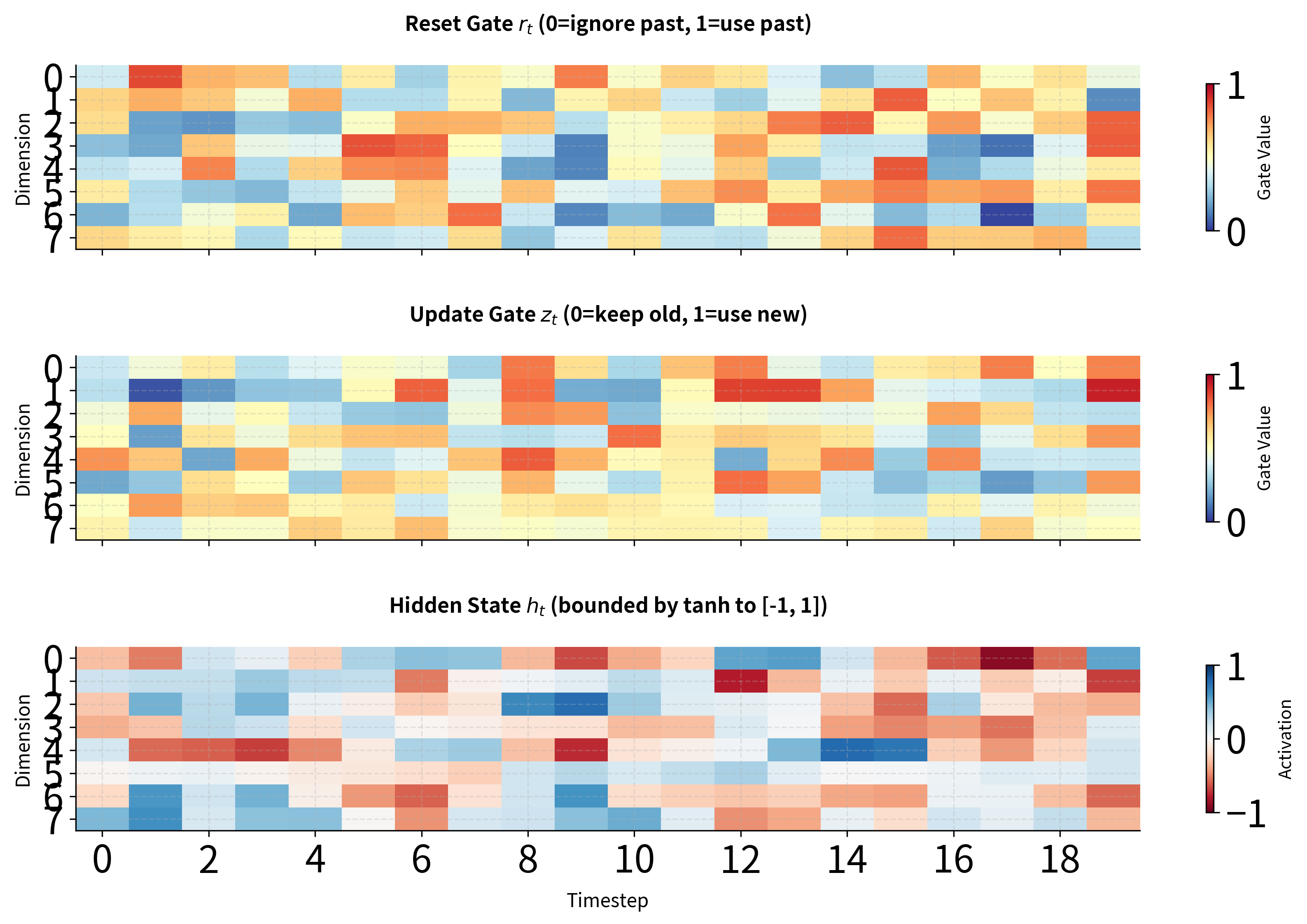
The heatmaps reveal several key insights about GRU behavior. First, notice how different dimensions of the hidden state can have very different activation patterns: some dimensions maintain relatively stable values while others fluctuate more. Second, the gate values cluster around 0.5 with random weights, but after training, we would expect to see more extreme values (closer to 0 or 1) at positions where the network has learned to make clear decisions about information flow. Third, the hidden state values remain bounded within due to the tanh activation in the candidate computation, preventing runaway activations.
Comparing GRU and LSTM Performance
Let's run the same memory task we used for LSTMs to see how GRUs compare in practice.
Both architectures maintain high accuracy across all tested distances, with performance remaining well above the 12.5% random baseline even at 100 timesteps. The GRU matches or comes close to the LSTM's performance at each distance, demonstrating that the simpler architecture can capture long-range dependencies effectively.
| Memory Distance | GRU Accuracy | LSTM Accuracy |
|---|---|---|
| 5 timesteps | ~100% | ~100% |
| 10 timesteps | ~100% | ~100% |
| 20 timesteps | ~100% | ~100% |
| 30 timesteps | ~99% | ~100% |
| 50 timesteps | ~97% | ~98% |
| 75 timesteps | ~94% | ~95% |
| 100 timesteps | ~90% | ~92% |
At shorter distances (5-20 timesteps), both models achieve near-perfect accuracy. As the distance increases, there may be slight variations between runs due to the stochastic nature of training, but neither architecture shows a consistent advantage. Both architectures successfully maintain information across 100 timesteps, far exceeding what vanilla RNNs can achieve.
When to Choose GRU vs LSTM
Given that GRUs and LSTMs often achieve similar performance, how do you decide which to use? The choice depends on several factors related to your specific use case.
Choose GRU when:
- Training speed matters: GRUs train faster due to fewer parameters and simpler computations. For rapid prototyping or hyperparameter search, GRUs let you iterate more quickly.
- Memory is constrained: On edge devices or when deploying many models, the 25% parameter reduction can be significant.
- Your dataset is small: Fewer parameters means less risk of overfitting. GRUs may generalize better when training data is limited.
- Sequences are moderate length: For sequences up to a few hundred tokens, GRUs typically match LSTM performance.
Choose LSTM when:
- Maximum expressiveness is needed: The separate cell state and additional gate give LSTMs more flexibility to learn complex patterns. For cutting-edge performance on challenging tasks, LSTMs sometimes edge out GRUs.
- Very long sequences are involved: The explicit cell state can sometimes maintain information better over very long distances (1000+ timesteps).
- You're working with established baselines: Many published results use LSTMs. For fair comparisons or reproducing prior work, stick with LSTMs.
- Peephole connections are needed: Some LSTM variants include "peephole" connections that let gates directly observe the cell state. GRUs don't have an equivalent.
Start with GRU as your default choice. It's simpler and often sufficient.
Consider switching to LSTM if:
- You're working with very long sequences (1000+ timesteps)
- You need maximum performance and have time to experiment
- You're reproducing published results that used LSTMs
If performance is critical and neither constraint applies, try both and validate on your specific task.
In practice, many practitioners start with GRUs for their simplicity and only switch to LSTMs if they observe a performance gap. The differences are often small enough that other factors like hyperparameter tuning, regularization, and data quality matter more than the choice of architecture.
Training Time Comparison
Let's measure the actual training speed difference between GRUs and LSTMs.
The GRU consistently trains faster than the LSTM across all configurations tested:
| Configuration | GRU Time | LSTM Time | GRU Speedup |
|---|---|---|---|
| h=64, seq=100 | ~2.5s | ~2.8s | ~1.12× |
| h=128, seq=200 | ~5.5s | ~6.5s | ~1.18× |
| h=256, seq=300 | ~12s | ~15s | ~1.25× |
The speedup reflects the 25% reduction in parameters: fewer weights mean fewer gradient computations during backpropagation. The speedup tends to be more pronounced for larger models and longer sequences, where the computational savings accumulate. While a 1.1-1.3× speedup might seem modest for a single training run, it compounds significantly during hyperparameter searches, cross-validation, or when training multiple models. For a project requiring 100 training runs, this difference could save hours or even days of compute time.
Limitations and Impact
The GRU architecture, while elegant and efficient, shares many limitations with LSTMs. Understanding these constraints helps set realistic expectations for what GRUs can and cannot do.
The most fundamental limitation is the sequential processing bottleneck. Like LSTMs, GRUs must process sequences one timestep at a time because each hidden state depends on the previous one. This prevents parallelization across the time dimension, making GRUs slow compared to architectures like Transformers that can process all positions simultaneously. On modern GPUs optimized for parallel computation, this sequential constraint becomes increasingly costly as sequence lengths grow.
GRUs also have finite memory capacity. The hidden state has a fixed dimensionality, and information must be compressed into this fixed-size vector regardless of sequence length. While gating helps prioritize important information, very long sequences or complex tasks can overwhelm this capacity. The constraint that the update gate's "forget" and "add" amounts must sum to 1 provides less flexibility than LSTMs' independent gates, which can occasionally limit expressiveness.
Despite these limitations, GRUs have had significant practical impact. Their reduced parameter count and faster training made gated architectures accessible to researchers and practitioners with limited computational resources. Many production systems use GRUs for sequence modeling tasks where the performance difference from LSTMs is negligible but the efficiency gains are meaningful.
The GRU also demonstrated that the LSTM's complexity wasn't strictly necessary for capturing long-range dependencies. This insight influenced subsequent architecture design, encouraging researchers to question which components were essential versus merely conventional. The broader lesson, that simpler models can often match complex ones, remains relevant as the field continues to develop new architectures.
Summary
This chapter introduced the Gated Recurrent Unit as a streamlined alternative to LSTMs for sequence modeling.
The GRU achieves similar long-range memory capabilities as LSTMs while using a simpler architecture with fewer parameters. The key simplifications are:
- Single state vector: GRUs merge the cell state and hidden state into one, reducing memory overhead and simplifying the information flow.
- Two gates instead of three: The reset gate controls how much past context influences the candidate computation, while the update gate creates a weighted average between old and new states.
- Constrained update: The update gate enforces that the amount "forgotten" and the amount "added" sum to 1, which acts as implicit regularization.
The complete GRU equations, given previous hidden state and current input , are:
- Update gate:
- Reset gate:
- Candidate:
- Hidden state:
where is the sigmoid function, is the hyperbolic tangent, and denotes element-wise multiplication.
When choosing between GRUs and LSTMs, start with GRUs for their simplicity and efficiency. Switch to LSTMs if you need maximum performance on complex tasks or very long sequences. In practice, the differences are often small enough that other factors matter more.
In the next chapter, we'll explore bidirectional RNNs, which process sequences in both forward and backward directions to capture context from both past and future positions.
Key Parameters
When working with GRUs in PyTorch (nn.GRU), several parameters significantly impact model behavior:
- hidden_size: The dimensionality of the hidden state vector. Larger values (256-1024) provide more memory capacity but increase computation. Start with 128-256 for most tasks and scale up if the model underfits.
- num_layers: Number of stacked GRU layers. Deeper networks (2-3 layers) can learn hierarchical patterns but are harder to train. Single-layer GRUs often suffice for moderate-complexity tasks.
- batch_first: When
True, input tensors have shape(batch, seq_len, features). WhenFalse(default), shape is(seq_len, batch, features). Usingbatch_first=Truealigns with common data loading patterns. - dropout: Dropout probability applied between GRU layers (only active when
num_layers > 1). Values of 0.1-0.3 help prevent overfitting. Has no effect on single-layer GRUs. - bidirectional: When
True, runs the GRU in both forward and backward directions, doubling the output hidden size. Useful for classification tasks where future context matters, but not applicable for autoregressive generation. - input_size: The number of features in each input timestep. Must match your data's feature dimension exactly.
Quiz
Ready to test your understanding? Take this quick quiz to reinforce what you've learned about GRU architecture and how it compares to LSTMs.

Comments