Attention Mechanism Intuition: Soft Lookup, Weights

In the encoder-decoder framework we covered in the Encoder-Decoder Framework chapter, the model compresses an entire input sequence into a single fixed-length vector. This works reasonably well for short sequences, but as inputs grow longer, that single vector becomes an information bottleneck. How can we expect one vector to faithfully represent a 50-word sentence, let alone an entire paragraph? The encoder's final hidden state must somehow encode every word, every phrase, every syntactic relationship, and all of this must fit into a vector of fixed size. The model is asked to perform an impossible compression: pour a gallon of meaning into a pint-sized vector.

Attention solves this by allowing the decoder to look back at all encoder states and decide which parts of the input are most relevant at each decoding step. Instead of relying on a compressed summary, the model learns to focus on different parts of the input as it generates each output token. This simple idea dramatically improved sequence-to-sequence models and became the foundation for the transformer architecture at the heart of modern NLP.

This chapter builds the intuition for how attention works: why it is needed, what it computes, how to interpret the results, and how different formulations compare. You will come away with a thorough understanding of attention as a general mechanism before we examine Bahdanau attention and Luong attention as concrete implementations in the following chapters.

To understand why attention matters, we need to understand the problem it solves. In a standard encoder-decoder model, an RNN reads the input sequence one token at a time, updating its hidden state at each step. After the final token, the hidden state is passed to the decoder as the context vector.

This design places a heavy burden on a single vector. Consider translating a 20-word English sentence to French. The encoder reads all 20 words and produces a single vector. The decoder then generates the French translation, one word at a time, relying entirely on that vector.

There are two fundamental problems with this approach. First, the vector has a fixed capacity regardless of input length. A 5-word sentence and a 50-word sentence both produce context vectors of the same size. Longer inputs must compress more information into the same space, inevitably losing detail. If you picture each dimension of the context vector as a filing cabinet drawer, you have the same number of drawers whether you are filing five documents or five hundred. Something must be thrown away or badly crumpled to fit.

Second, information from early in the sequence must survive many RNN steps to reach the final hidden state. The vanishing gradient problem (explored in the Vanishing Gradients chapter) makes this difficult: gradients shrink exponentially as they propagate backward through many time steps, which means the encoder's parameters receive little signal about how to preserve early-sequence information. The context vector ends up dominated by information from the end of the input.

These two problems compound each other. Longer sequences demand more compression while simultaneously making it harder to retain early content. The empirical evidence was striking: in the years before attention, researchers consistently found that seq2seq translation quality peaked around 10 to 15 tokens and degraded sharply beyond 20 to 30 tokens. The measured decline showed that the bottleneck limited performance.

Attention addresses both problems at once. Instead of relying on a single final state, the decoder can access all encoder hidden states at every generation step. The model learns to weight these states dynamically, giving more attention to whichever encoder positions are most useful for generating the current output token.

To make the bottleneck concrete, imagine the encoder processing "The quick brown fox jumped over the lazy dog." The encoder's final hidden state must carry useful information about all nine words: the subject (fox), its modifiers (quick, brown), the verb (jumped), the preposition (over), and the object (dog) with its modifier (lazy). As the decoder generates the translation word by word, it relies entirely on this single vector for the entire sentence.

The decoder begins by generating the equivalent of "The." For this, it needs information about "The" from the encoder. Then it generates the adjective for "quick" and "brown," needing those features. By the time it reaches "dog" and "lazy," nine decoding steps later, the context vector has not changed at all; it is still the same compressed representation from the beginning. This static context vector is the bottleneck. The decoder must extract all of its needed information from one frozen vector, using it for every single generation step, regardless of where in the output it currently finds itself.

Attention shifts the problem from "compress everything into one vector" to "learn which parts are relevant right now." The latter is a much easier learning problem because it is local and specific. Rather than asking the encoder to pack every fact about a sentence into a single representation, attention lets the decoder pick up the relevant fact when it needs it.

Think of the difference between reading a book once and trying to answer questions from memory versus having the book open and being able to flip to relevant pages as you answer each question. The first approach places enormous demands on memory. The second approach makes each question easier by providing direct access to the relevant information. Attention is the second approach: the encoder states are the open book, and the attention mechanism is the ability to flip to the right page at each step.

Think of attention as a soft, differentiable dictionary lookup. In a traditional dictionary, you provide a key and get back exactly one value. Attention works similarly, but instead of retrieving a single value, it retrieves a weighted combination of all values based on how well each key matches your query.

Consider a translation task where you're generating the French word for "cat" from an English sentence. Rather than searching through the entire compressed representation, attention lets the decoder ask: "Which parts of the input are most relevant right now?" The answer comes as a probability distribution over all input positions.

The mechanics involve three components:

• The query represents what we are currently looking for. In encoder-decoder attention, this is the decoder's current hidden state.
• The keys represent what we're comparing against. These are the encoder's hidden states, one per input position.
• The values represent what we retrieve once we find a match. In basic attention, keys and values are the same encoder hidden states, though they can be separate learned projections.

The attention mechanism computes similarity scores between the query and all keys, normalizes these scores into a probability distribution using softmax, and returns a weighted sum of the values. This weighted sum is the context vector that the decoder uses alongside its own state to generate the next token.

The analogy to information retrieval is revealing. When you search a database, you have a query (what you are looking for) and you compare it against a set of keys (indexed fields). When you find a match, you retrieve the associated value (the full record). Attention makes this process soft and continuous: instead of a hard match, every key partially matches the query, and you retrieve a blend of all values weighted by match quality. This connection to information retrieval is not coincidental. Scaled dot product attention, the variant used in transformers, was explicitly designed to mirror this structure, as we'll see in upcoming chapters.

The query-key-value framing deserves close attention because it underpins every modern attention mechanism, from the original Bahdanau variant to the transformers that power today's language models. Understanding this framing deeply will make every subsequent chapter easier.

Imagine you are in a library with a very helpful librarian. You walk in and say "I'm looking for books about the French Revolution" (your query). The librarian looks through the catalog cards (the keys), which are brief descriptions of each book. They find three cards with high similarity to your query: one for a general history, one for a biography of Robespierre, and one on the economic causes of the revolution. They retrieve those books (the values) and bring them to you, with the most relevant book on top.

In this analogy, the catalog cards (keys) are compact representations designed for efficient comparison, while the books themselves (values) contain the content you need. This separation of roles is architecturally meaningful. You want the comparison (query against key) to be efficient and well-calibrated, while the retrieval (values) can be richer and more complex.

In basic seq2seq attention, keys and values are both just the encoder hidden states, so the distinction collapses. But in transformer self-attention, keys and values are separate learned projections of the same encoder states, allowing the model to optimize comparison separately from content retrieval. We will explore this separation fully in the Self-Attention chapter.

For now, the essential intuition is this: the query captures "what I need," the keys capture "what each position offers for comparison," and the values capture "what each position contributes." Attention computes the match between query and keys, then uses that match to blend the values.

Now that we have the intuition, let's translate it into precise mathematics. The goal is to build a mechanism that answers one question at each decoding step: "Which parts of the input should I focus on right now?"

Imagine you're the decoder, trying to generate the next word in a translation. You have your current state $s_t$, which encodes what you've generated so far and what you're trying to produce next. Meanwhile, the encoder has processed the entire input sentence and produced a sequence of hidden states $h_1, h_2, \ldots, h_T$, one for each of the $T$ input words. Each encoder state $h_j$ captures the meaning of word $j$ in context.

The challenge is clear: you need to selectively combine information from all these encoder states, giving more weight to positions that are relevant to your current generation task. Attention solves this in three steps.

The first question attention must answer is: "How relevant is each input position to what I'm currently generating?" We need a way to compare the decoder's current state with each encoder state and produce a relevance score.

This comparison happens through a scoring function:

where:

• $e_{tj}$: the alignment score, a single number indicating how relevant encoder position $j$ is when generating at decoder position $t$
• $s_t$: the decoder's hidden state at step $t$, encoding the generation context
• $h_j$: the encoder's hidden state at position $j$, encoding information about input word $j$
• $\text{score}(\cdot, \cdot)$: any function that takes two vectors and returns a scalar measuring their compatibility

Think of this as the decoder asking each encoder position: "How useful are you for what I'm trying to do right now?" A high score means "very useful," while a low or negative score means "not relevant."

What should this scoring function look like? The simplest choice is the dot product: $e_{tj} = s_t^\top h_j$, which measures how aligned the two vectors are in the embedding space. Vectors pointing in similar directions yield high scores; orthogonal vectors yield zero. We'll explore more sophisticated scoring functions in the section on attention formulations below, and cover them in full detail in the Bahdanau Attention and Luong Attention chapters.

The decoder state $s_t$ deserves a closer look. In an RNN decoder, $s_t$ is the hidden state at generation step $t$, after the decoder has already generated tokens $y_1, y_2, \ldots, y_{t-1}$. It carries information about both what has been generated and what the decoder is about to produce. This duality is why $s_t$ makes a good query: it simultaneously knows what context has already been established (so it doesn't ask the encoder to repeat what was already encoded in earlier context vectors) and what needs to be generated next (so it can seek out the relevant encoder information for the upcoming token).

Raw alignment scores present a problem: they can be any real number, positive or negative, large or small. We need to convert them into something interpretable and usable, specifically a probability distribution over input positions.

The softmax function accomplishes this transformation. Given the alignment scores $e_{t1}, e_{t2}, \ldots, e_{tT}$ for all $T$ input positions, the attention weight for position $j$ is:

where:

• $\alpha_{tj}$: the attention weight for position $j$, guaranteed to be between 0 and 1
• $\exp(e_{tj})$: the exponential function applied to the alignment score, converting any real number to a positive value
• $\sum_{k=1}^{T} \exp(e_{tk})$: the sum of all exponentiated scores, serving as a normalizing constant

Why softmax? The exponential function maps any real number to a positive value. This ensures all weights are non-negative. Dividing by the sum of all exponentials guarantees that $\sum_{j=1}^{T} \alpha_{tj} = 1$. The result is a valid probability distribution over input positions.

Softmax also has a useful amplification property. If one score is much larger than the others, its corresponding weight will dominate. For example, if $e_{t1} = 5$ and all other scores are near 0, then $\alpha_{t1}$ will be close to 1 while the other weights approach 0. This allows the model to focus sharply on a single position when appropriate, or spread attention across multiple positions when relevance is more evenly distributed.

The competition enforced by softmax is worth dwelling on. Because all weights must sum to 1, increasing attention to one position automatically decreases attention to others. This makes attention a zero-sum competition for relevance: every additional unit of focus on position $j$ is taken from other positions. As a result, training the model to focus correctly on position $j$ requires rewarding high scores for $j$ while learning to suppress all positions that are less relevant. This competitive dynamic helps attention produce sharp, interpretable patterns rather than diffuse or arbitrary distributions.

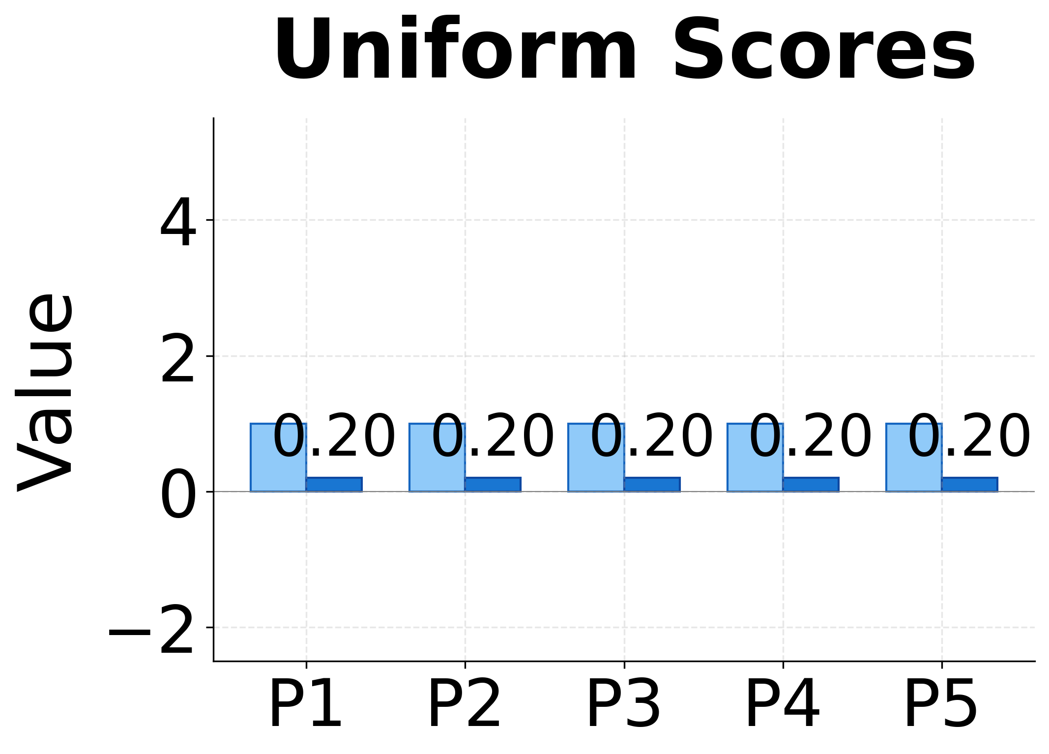
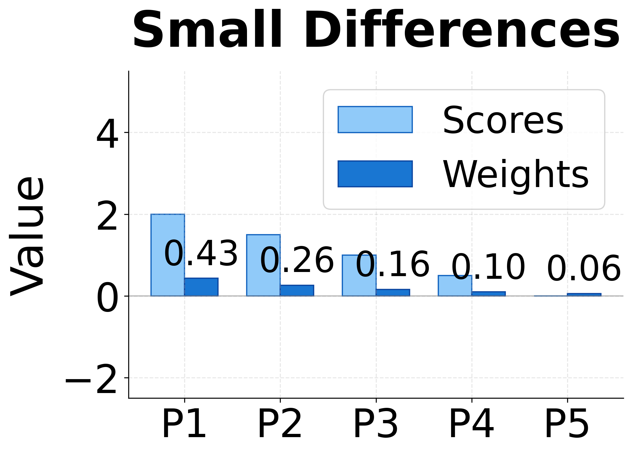
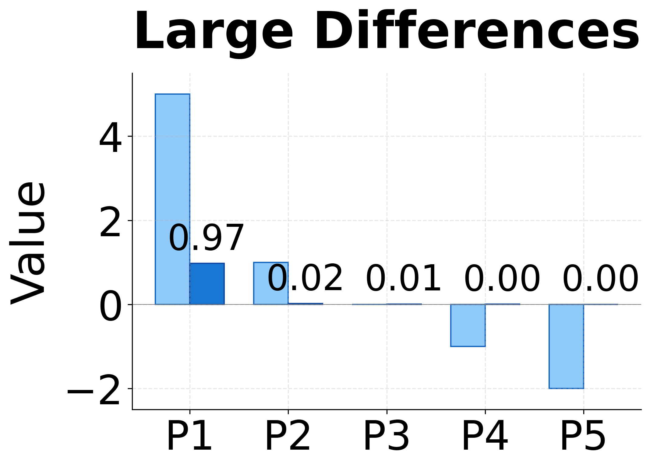
The visualization above demonstrates this amplification effect. With uniform scores, softmax produces uniform weights (0.20 each). Small score differences get amplified into clearer preferences. Large differences produce nearly one-hot attention, where almost all weight concentrates on the highest-scoring position.

With attention weights in hand, we can finally answer our original question: "What information from the input should I use?" The answer is a weighted combination of all encoder states:

where:

• $c_t$: the context vector at decoder step $t$, a single vector summarizing the relevant input information
• $\alpha_{tj}$: the attention weight for encoder position $j$ at decoder step $t$
• $h_j$: the encoder hidden state at position $j$ (the "value" being retrieved)

This weighted sum is the heart of attention. Each encoder state contributes to the context vector in proportion to its attention weight. If $\alpha_{t3} = 0.7$ and all other weights are small, then $c_t$ will be dominated by $h_3$, the information at position 3. If weights are more evenly spread, the context vector blends information from multiple positions.

The context vector has the same dimension as the encoder states, making it easy to integrate with the rest of the model. The decoder uses $c_t$ alongside its own state $s_t$ to predict the next output token, often by concatenating them and passing through a feed-forward layer. The standard approach concatenates them as $[c_t; s_t]$ and passes the combined vector through a learned transformation followed by a softmax over the vocabulary.

One subtle but important property of this formula is that the context vector is always the same dimension as the encoder states, regardless of $T$, the number of input positions. Whether we are weighting 5 encoder states or 500, the result is always a single vector of dimension $d_h$. This is what gives attention its elegant scalability: adding more input tokens does not change the interface between attention and the rest of the model.

Let's trace through a concrete example. Suppose we're translating "The cat sat" and currently generating the French word "chat" (cat). The decoder state $s_t$ encodes that we've generated "Le" and are now producing the noun.

1. Alignment scores: The scoring function compares $s_t$ with each encoder state. It finds high compatibility with $h_2$ (the representation of "cat") and lower compatibility with $h_1$ ("The") and $h_3$ ("sat").

2. Attention weights: Softmax converts these scores into probabilities. Perhaps $\alpha_{t1} = 0.05$, $\alpha_{t2} = 0.85$, $\alpha_{t3} = 0.10$.

3. Context vector: The weighted sum $c_t = 0.05 \cdot h_1 + 0.85 \cdot h_2 + 0.10 \cdot h_3$ produces a context vector dominated by the representation of "cat."

The decoder combines $c_t$ with $s_t$ and predicts "chat" as the next word. At the next step, when generating "noir" (black), the attention mechanism shifts focus to the encoder state for "black." This dynamic, step-by-step focus is what makes attention effective. Rather than relying on a single compressed representation of the entire input, the model can look back at the original encoder states and select the information most relevant to each generation step.

Notice that this also handles an important linguistic phenomenon: reordering. In French, adjectives typically follow the noun, so "black cat" becomes "chat noir." Without attention, the decoder would have to somehow use a single compressed vector to generate words in a different order than the input. With attention, the decoder simply attends to "cat" when generating "chat" and to "black" when generating "noir," regardless of the fact that these words appeared in reverse order in the source. Attention handles word reordering naturally because it is agnostic to position, caring only about relevance.

Understanding attention in isolation is one thing; understanding how it connects to the full decoding process is another. Let's trace through the entire decoder step in detail, seeing exactly how the context vector feeds into the generation of each output token.

At each decoding step $t$, the decoder maintains a hidden state $s_t$ and must produce two things: the next output token and the updated hidden state for the next step. The attention mechanism intervenes between these two operations, enriching the decoder's information before it makes the prediction.

The standard decoder with attention follows this sequence at each step $t$:

First, the decoder receives two inputs: the embedding of the previously generated token $y_{t-1}$ and the previous context vector $c_{t-1}$. These are concatenated and fed into the RNN cell together with the previous hidden state $s_{t-1}$:

Next, the new decoder state $s_t$ is used to compute attention over the encoder states, producing a fresh context vector $c_t$ tailored to the current generation step:

Finally, $s_t$ and $c_t$ are combined to predict the output token. A common approach is to concatenate them, apply a linear transformation to produce a pre-output vector $\tilde{s}_t$, and then apply softmax over the vocabulary:

where $W_c$ and $W_v$ are learned weight matrices. This is the architecture used in Luong attention, which we will study in detail in the Luong Attention chapter.

There is a noteworthy design choice in how the decoder state is computed. Some implementations, including Bahdanau's original formulation, compute attention using $s_{t-1}$ (the previous decoder state) rather than $s_t$ (the current one). Using $s_{t-1}$ for attention means the model selects its focus before integrating the previous output token, while using $s_t$ means the focus is informed by the current token's embedding. Both approaches work in practice, with Bahdanau using $s_{t-1}$ and Luong using $s_t$.

The full decoder loop creates an interesting feedback structure. The context vector $c_t$ influences what token is generated. That generated token becomes the input for the next step, which influences the new decoder state $s_{t+1}$, which in turn shapes the next attention distribution. Attention is not a one-shot computation; it participates in a dynamic, step-by-step dialogue between the decoder and the encoder states.

This feedback loop is why attention is so powerful for generation tasks. When the decoder generates accurate translations early in the output by focusing well, it creates a good hidden state for the next step. That good hidden state produces a better query for attention, which produces a better context vector, and so on. Conversely, when the decoder makes an error, that error can propagate forward through the hidden state, making subsequent attention queries less accurate. This is one reason why beam search (maintaining multiple hypotheses in parallel) is useful: it hedges against early errors by not committing to a single generation path.

To cement the mechanics, let's walk through attention computation for a complete sentence, step by step, with concrete numbers.

We will use the translation of "The cat sat" to French, simplified to focus on the attention computation. The encoder has processed the English sentence and produced three hidden states:

These are 2-dimensional vectors to keep the arithmetic readable. In practice they would be hundreds of dimensions.

Step t=1: Generating "Le" (The)

The decoder starts with an initial state $s_1 = [0.7, 0.3]$ (encoding "start of translation, producing an article").

Alignment scores using dot product:

Applying softmax to get attention weights (using $\exp$ of each score divided by the sum):

Context vector (weighted sum of encoder states):

The attention is fairly distributed here, which makes sense for generating an article: "Le" is mostly determined by the subject noun ("cat"), but generating it requires knowing the overall sentence structure.

Step t=2: Generating "chat" (cat)

After generating "Le," the decoder advances to state $s_2 = [0.2, 0.8]$ (now oriented toward producing the noun). The attention query shifts dramatically toward $h_2$:

The score for position 2 ("cat") is now much higher. After softmax:

Now over half the attention weight falls on "cat." The context vector $c_2$ will be dominated by $h_2$. This provides the decoder with a strong signal about the noun to generate.

Step t=3: Generating the verb

For the verb phrase, the decoder state would shift again to attend primarily to $h_3$ ("sat"). This illustrates how attention tracks the linguistic content being generated at each step, automatically shifting focus as the translation proceeds through different parts of the source sentence.

This step-by-step trace reveals something important: the attention weights are not predetermined. They emerge from the interaction between the decoder's current state and the encoder states at each step. As the decoder evolves through the translation, its internal state changes, and those changes shift which encoder positions receive high attention. The mechanism is fully dynamic, computed fresh at every generation step.

Attention weights offer something rare in deep learning: interpretability. By examining which input positions receive high attention weights, we can understand what the model is "looking at" when making each prediction.

In machine translation, attention weights often reveal meaningful alignments between source and target languages. When translating "The black cat sat on the mat" to French "Le chat noir etait assis sur le tapis", the model typically attends to "cat" when generating "chat", "black" when generating "noir", and "mat" when generating "tapis." This alignment emerges automatically from training, without any explicit supervision about word correspondences.

The alignment patterns that emerge often match what a linguist would predict. Subject-verb-object structures tend to produce diagonal attention matrices for languages with similar word order. Cross-linguistic reorderings, such as the adjective-after-noun convention in French, produce off-diagonal patterns where target tokens attend to source positions in a different order. The model discovers these patterns without being told anything about grammar or syntax; it learns them because they help minimize translation loss.

However, attention weights require careful interpretation. Several caveats apply:

• Weights show correlation, not causation: High attention on a position doesn't mean that position caused the output. It means the model found that position useful, but the relationship may be indirect. A model translating "not happy" might attend heavily to "not" while generating the translation, but the actual semantic work of understanding negation is distributed across many layers and weights in the network.
• Distributed information: Important information might be spread across multiple positions with moderate weights. Focusing only on the highest-weight position misses the full picture. Some linguistic relationships, such as long-distance agreement, require integrating information from multiple positions simultaneously.
• Layer effects: In multi-layer models, different layers may attend to different aspects of the input. Shallow layers often capture local structure while deeper layers capture longer-range dependencies.
• Head specialization: In multi-head attention, different heads often specialize in different types of relationships. One head might track positional adjacency, another might track syntactic dependencies, and another might track semantic similarity. Visualizing only one head can give a misleading picture of what the model has learned.

Despite these caveats, attention visualization remains one of the most valuable tools for understanding model behavior and debugging unexpected predictions. When a translation is wrong, plotting the attention heatmap often reveals immediately whether the model attended to the wrong source position, skipped a word, or duplicated coverage. This transparency helped practitioners diagnose errors and contributed to attention's rapid adoption.

Attention heatmaps place source tokens on one axis and target tokens on the other, with cell intensity representing the attention weight. A few patterns are worth knowing:

A near-diagonal pattern indicates that the source and target languages have similar word order, and the model is generating the translation in roughly the same order as the source. This is common for closely related languages like English and German or Spanish and Italian.

Vertical stripes indicate that the same source position receives high attention across many target steps. This often corresponds to source tokens that influence many target words, such as articles, auxiliary verbs, or punctuation that triggers systematic differences between languages.

Horizontal stripes indicate that a specific target token attends broadly across many source positions. This can occur when generating punctuation, discourse markers, or words whose meaning depends on the global context rather than a specific source word.

One of attention's most practical benefits is graceful handling of variable-length sequences. Traditional encoder-decoder models compress inputs of any length into a fixed-size vector, creating a fundamental mismatch: longer inputs must squeeze more information into the same space.

Attention sidesteps this entirely. The context vector $c_t$ is always a weighted average of encoder states, regardless of sequence length. For a 10-word sentence, we average over 10 states. For a 100-word paragraph, we average over 100 states. The mechanism scales naturally because the weighted sum always produces a vector of the same dimension as the encoder states.

This property is important for tasks with highly variable input lengths:

• Document summarization: Articles range from a few sentences to thousands of words
• Question answering: Questions are short, but context passages can be lengthy
• Code generation: Function descriptions vary from one-liners to detailed specifications

Without attention, longer inputs would require either truncation (losing information) or larger hidden states (increasing memory and computation). Attention avoids both problems by dynamically selecting relevant information at each step, regardless of where in the sequence that information lives.

There is a subtle but important consideration here. While attention handles variable-length inputs gracefully at the context vector level, the RNN encoder itself still must process the entire input sequentially. For very long sequences, the RNN hidden states may still carry degraded information from positions that are many steps back. Attention allows the decoder to retrieve any encoder state, but if that encoder state itself doesn't carry good information because the RNN couldn't propagate it well, the retrieval doesn't help much. This is one reason why bidirectional encoders are common in attention models: by running the RNN in both directions and concatenating the resulting states, each encoder position benefits from context both preceding and following it, reducing the degradation problem.

Before attention became widespread, sequence models often used pooling operations to aggregate information. Mean pooling averages all hidden states, while max pooling takes the element-wise maximum. Understanding how attention differs from these simpler approaches clarifies exactly what attention adds.

Mean pooling treats all positions equally by computing a simple average:

where:

• $c$: the aggregated context vector, the same dimension as hidden states
• $T$: the number of positions in the sequence
• $h_j$: the hidden state at position $j$

Each position receives weight $\frac{1}{T}$, regardless of content. This works when all parts of the input contribute equally to the output, but fails when relevance varies. In sentiment analysis, the phrase "not good" carries more weight than "the movie was", yet mean pooling gives them equal importance.

Max pooling extracts the strongest signal at each dimension independently:

where:

• $c_d$: the $d$-th dimension of the aggregated vector
• $h_{jd}$: the $d$-th dimension of the hidden state at position $j$
• $\max_j$: the maximum value across all positions $j = 1, \ldots, T$

This captures salient features by selecting the most activated value for each dimension. However, it loses information about which positions contributed and cannot combine graded contributions from multiple positions.

Attention provides learned, context-dependent weighting:

where the weights $\alpha_{tj}$ are computed dynamically based on what the model needs at each step $t$. Unlike mean pooling's uniform weights or max pooling's binary selection, attention learns which positions matter most for the current prediction.

Consider the sentence "The movie was absolutely terrible" for sentiment classification. The comparison below shows how mean pooling and a trained attention mechanism would weight each word:

The contrast is stark. Mean pooling treats "The" and "terrible" as equally important, diluting the sentiment signal. Attention learns to focus on "terrible" and to a lesser extent "absolutely", producing a context vector that emphasizes the words driving the classification.

One more consideration separates attention from both pooling methods: attention is query-dependent. The same input sequence produces different context vectors at different decoding steps, because the query (decoder state) changes. Mean pooling and max pooling produce the same aggregation regardless of what you are trying to do with it. Attention adapts. When generating "chat" (cat), the attention mechanism focuses on the source position for "cat." When generating "noir" (black), it shifts focus to "black." This step-specific adaptation is something that pooling simply cannot provide.

The mathematics of attention translates directly into code. Let's implement the three-step process: compute alignment scores, apply softmax to get attention weights, and produce a context vector through weighted summation.

This verbose version makes it easy to audit each step individually. Notice that the numerical stability trick (subtracting the maximum score before exponentiating) does not change the final weights; it prevents overflow errors when dealing with very large raw scores, which is especially important when scores can reach values like 20 or 30 in high-dimensional spaces.

Attention weights are typically visualized as heatmaps, with rows representing decoder steps (outputs) and columns representing encoder positions (inputs). The resulting matrix provides an intuitive view of what the model focused on when generating each output token.

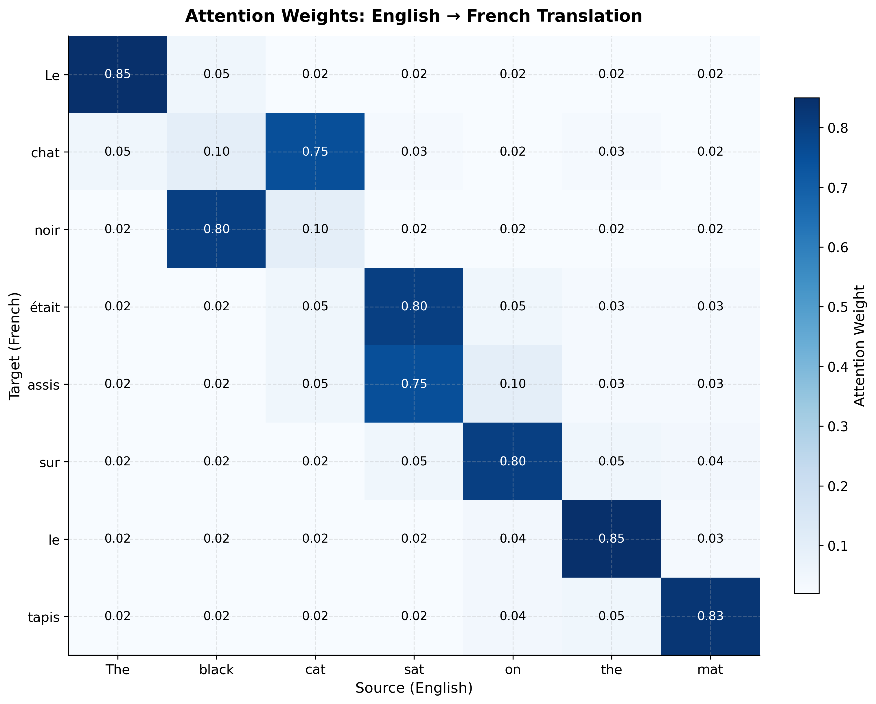
Several patterns emerge from this visualization:

• Diagonal tendency: Many languages share similar word order, so attention often follows a rough diagonal path from upper-left to lower-right
• Reordering: French adjectives follow nouns ("chat noir" vs "black cat"), visible in the swapped attention for "chat" (attending to "cat") and "noir" (attending to "black")
• Many-to-one mapping: Both "etait" and "assis" attend primarily to "sat", which reflects how French uses two words where English uses one
• Article alignment: Function words like "Le" and "le" align with their English counterparts

This kind of alignment matrix became a key piece of evidence in the original Bahdanau et al. (2014) paper showing that attention had learned meaningful linguistic structure without explicit supervision. The heatmaps showed structured, interpretable correspondences that matched human linguistic intuition rather than leaving the translation process entirely opaque.

To see attention in a more complete context, let's build a simple attention-based classifier for sentiment analysis. This shows how attention identifies which words drive the prediction.

Since this is an untrained model with randomly initialized weights, the attention distribution appears arbitrary. After training on labeled sentiment data, we would expect sentiment-bearing words like "great", "terrible", "loved", and "hated" to receive substantially higher attention weights (0.5 to 0.8), while function words like "the" and "was" would receive minimal attention (0.02 to 0.10).

What would attention look like in a trained model? The table below shows realistic attention patterns for four sentiment sentences:

These patterns reveal what we would expect:

• Sentiment words dominate: "great", "terrible", and "loved" receive the highest weights
• Negation matters: In "not great", both "not" and "great" receive significant attention, as the model must combine them to understand the negated sentiment
• Function words ignored: Words like "the" and "was" consistently receive low attention

The negation case deserves special emphasis. Negation is notoriously difficult for bag-of-words models because the word "great" has a positive sentiment regardless of context. A model that attends to "not" alongside "great" has implicitly learned that negation modifies the adjacent sentiment word, even though the model was only trained on sentiment labels, not on any explicit representation of negation. This is attention learning linguistic structure from raw data, which is exactly the kind of emergent behavior that made researchers excited about it in 2014 and remains impressive today.

We've established that attention requires a scoring function to measure relevance between decoder and encoder states. Different choices lead to different attention mechanisms, each with distinct trade-offs.

The fundamental question each scoring function answers is the same: "Given what I'm trying to generate (the decoder state) and what information is available (an encoder state), how compatible are they?" The answer is always a single number, the alignment score. But how we compute that number varies significantly.

The most direct approach treats compatibility as geometric alignment. Two vectors pointing in similar directions have high compatibility; orthogonal vectors have zero compatibility. The dot product captures exactly this intuition:

where:

• $s_t$: the decoder state at step $t$, a vector of dimension $d$
• $h_j$: the encoder state at position $j$, also dimension $d$
• $s_t^\top h_j$: the inner product, computed as $\sum_{i=1}^{d} s_{t,i} \cdot h_{j,i}$

Geometrically, the dot product equals $\|s_t\| \cdot \|h_j\| \cdot \cos(\theta)$, where $\theta$ is the angle between the vectors. When both vectors point in the same direction ($\theta = 0$), the score is maximized. When they are perpendicular ($\theta = 90^\circ$), the score is zero.

This simplicity is both a strength and a limitation. Dot product attention requires no learnable parameters, making it computationally efficient. However, it requires the decoder and encoder to have the same hidden dimension, and it assumes compatibility can be measured purely through geometric alignment in the shared representation space. If the encoder and decoder use different architectures or different hidden sizes, dot product scoring cannot be applied without first projecting one into the other's space.

What if simple geometric alignment isn't expressive enough? Perhaps compatibility depends on complex, nonlinear relationships between the decoder and encoder states. Additive attention addresses this by introducing a small neural network:

where:

• $W_s$: a learnable weight matrix of dimension $d_a \times d_s$ that projects the decoder state
• $W_h$: a learnable weight matrix of dimension $d_a \times d_h$ that projects the encoder state
• $v$: a learnable weight vector of dimension $d_a$ that produces the final scalar score
• $\tanh$: the hyperbolic tangent, introducing nonlinearity
• $d_a$: the attention hidden dimension, a hyperparameter

The formula works as follows: $W_s s_t$ projects the decoder state into a new space of dimension $d_a$. Similarly, $W_h h_j$ projects the encoder state into the same space. Adding these projections combines information from both states. The $\tanh$ activation introduces nonlinearity. Finally, $v^\top$ projects the combined representation to a scalar score.

This approach has two key advantages. First, the learnable parameters allow the model to discover what "compatibility" means for the specific task. The network can learn to ignore certain dimensions of the encoder or decoder state, to focus on dimensions that are systematically predictive of relevance, and to capture interaction effects between specific encoder and decoder features. Second, since we project both states into a common space of dimension $d_a$, the encoder and decoder can have different dimensions. We'll implement this fully in the Bahdanau Attention chapter.

The cost is additional parameters: $d_a \times d_s$ (for $W_s$) plus $d_a \times d_h$ (for $W_h$) plus $d_a$ (for $v$). For a typical setup with $d_a = 128$, $d_s = 256$, and $d_h = 256$, this adds about 66,000 parameters. Compared to the millions of parameters in the LSTM layers, this is modest. But the scoring function must also be evaluated at every encoder position for every decoder step, so its computational cost scales with sequence length.

The transformer architecture revived dot product attention but added a scaling refinement. The problem with vanilla dot products becomes apparent in high dimensions: scores can grow very large, causing softmax to produce extremely peaked distributions.

To understand why, consider what happens when we compute $s_t^\top h_j$ for vectors with $d_k$ dimensions. If each component is independently drawn from a zero-mean, unit-variance distribution, the variance of the dot product is approximately $d_k$. For $d_k = 512$, the standard deviation of scores is about 22. Scores this large cause softmax to assign nearly all probability mass to a single position, producing near-zero gradients for all other positions and slowing learning. The model gets "stuck" because the peaked softmax means nearly all gradient signal goes to the single highest-scoring position; the other positions receive almost no gradient and cannot improve.

Scaled dot product attention fixes this by normalizing:

where:

• $d_k$: the dimension of the key vectors
• $\sqrt{d_k}$: the scaling factor that brings variance back to approximately 1 regardless of dimension

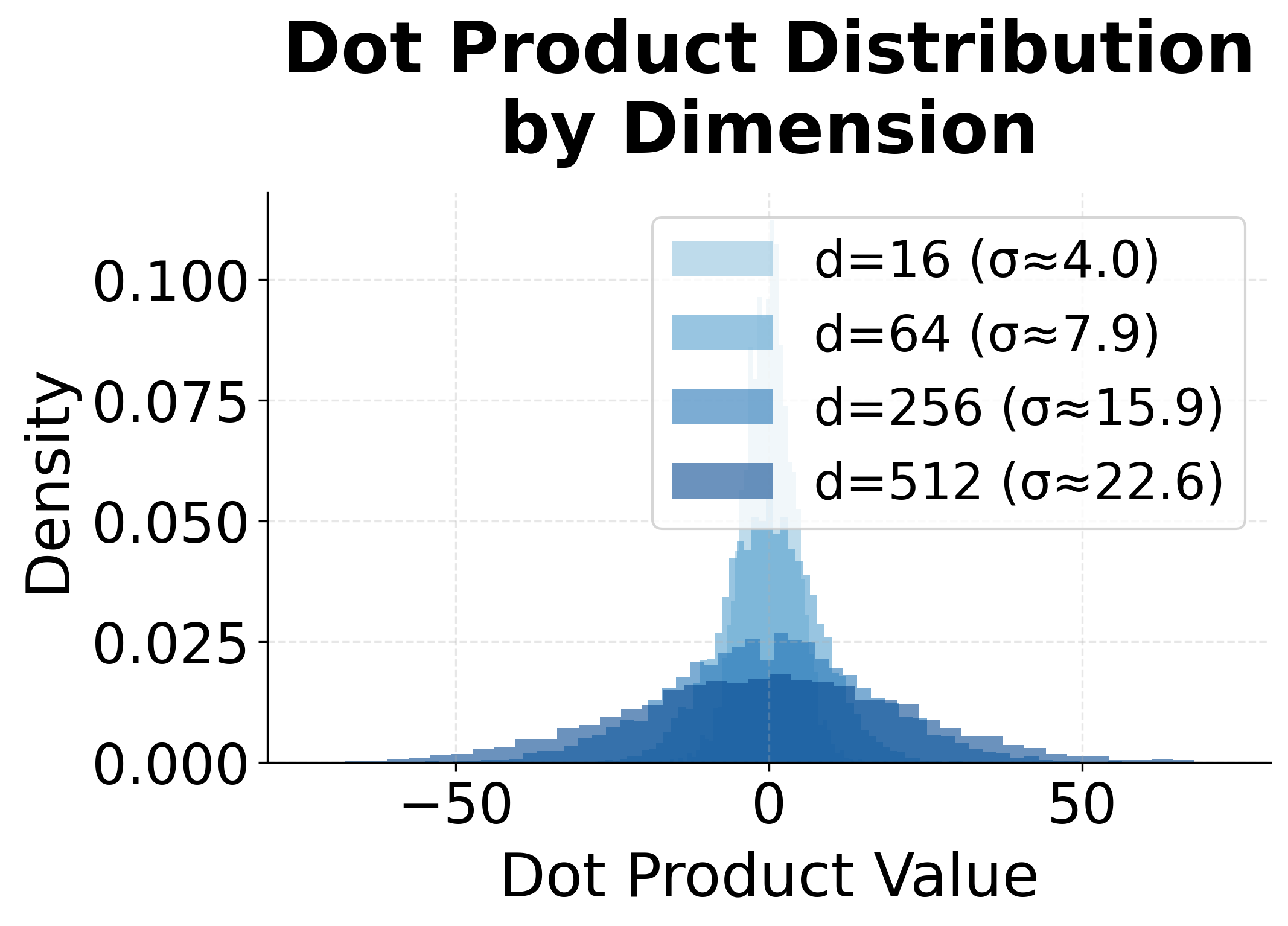
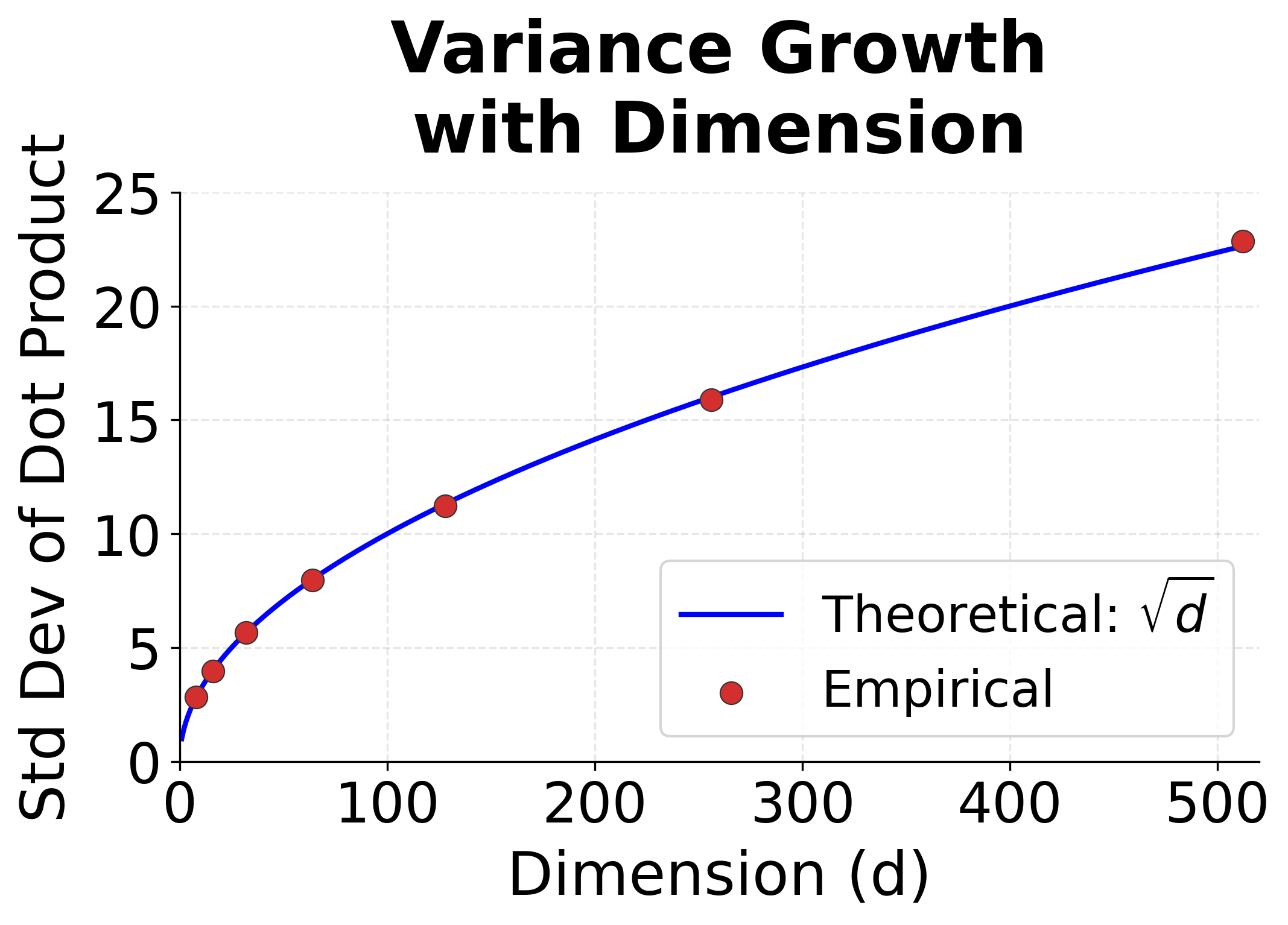
The visualization confirms the scaling problem. As dimension increases, the distribution of dot product scores spreads dramatically. At $d=512$, scores routinely exceed $\pm 40$, which would cause softmax to produce extremely peaked distributions. Scaling by $\sqrt{d_k}$ normalizes this spread back to a manageable range, keeping the standard deviation near 1 regardless of embedding dimension. This simple fix makes scaled dot product attention stable across a wide range of hidden dimensions and is one reason why transformers could be scaled to very large sizes without requiring careful tuning of the attention mechanism.

Each approach represents a different trade-off:

Dot product attention is fastest but requires matching encoder and decoder dimensions. Additive attention is most flexible and introduces learned parameters, at the cost of more computation per position. Scaled dot product combines the efficiency of dot products with numerical stability for high dimensions.

In modern practice, scaled dot product attention dominates. Its efficiency allows transformers to run multiple attention heads in parallel, each learning different aspects of relevance. The lack of learnable parameters in the score function is offset by the projection matrices that create queries, keys, and values. When you apply a linear projection to the encoder states before computing attention, you are effectively learning the alignment metric, just in a different, more modular way. We'll explore this architecture in the Self-Attention chapters.

One of attention's most important properties is that it is fully differentiable. The entire computation, from input through encoder, through attention scoring and weighting, through the context vector, through the decoder, to the output prediction, can be differentiated with respect to every parameter. This means attention can be trained end-to-end with standard gradient descent and backpropagation, with no need for separate training procedures or approximations.

The gradient flows through the attention mechanism in an illuminating way. The loss function (typically cross-entropy between the predicted and actual next token) computes a gradient with respect to the context vector $c_t$. This gradient propagates backward through the weighted sum formula:

The first equation says that the gradient with respect to encoder state $h_j$ is proportional to the attention weight $\alpha_{tj}$. Positions that received high attention get stronger gradient signal, which means the encoder is trained to produce representations that are useful for the specific alignments the attention mechanism chose. This creates a virtuous cycle: attention learns which encoder positions are relevant, and the encoder learns to make those positions informative for the expected attention pattern.

The second equation says that the gradient with respect to the attention weights is proportional to the encoder states. This gradient then flows back through the softmax and the scoring function, updating whatever parameters are involved in computing alignment scores. If you use additive attention with learned parameters $W_s$, $W_h$, and $v$, those parameters receive gradients that push them toward scoring the "right" positions more highly on future examples.

This end-to-end training property is what makes attention a principled machine learning mechanism rather than a hand-crafted feature. The model learns the alignment from data. No human annotates which source words correspond to which target words; the training signal comes entirely from whether the final translation was correct, and the gradient machinery propagates that signal all the way back to the alignment decisions.

The attention mechanism was introduced by Bahdanau et al. in their 2014 paper "Neural Machine Translation by Jointly Learning to Align and Translate." The motivation came directly from the bottleneck problem: translation quality degraded significantly as input length increased, exactly what you'd expect when compressing long sequences into a fixed-size vector.

Their solution was elegant: rather than compressing all information upfront, let the decoder decide what to look at. At each decoding step, the model learned to "align" the current output position with one or more input positions, dynamically constructing a context vector from those aligned positions. The paper included visualizations showing learned alignment matrices that closely matched linguistic intuitions about word correspondences between languages. These visualizations were striking because they suggested the model had discovered linguistically meaningful structure entirely from translation data, without any explicit alignment supervision.

The idea proved immediately impactful. Within months of the preprint appearing, attention mechanisms were being incorporated into a wide range of seq2seq models. Luong et al. (2015) explored alternative scoring functions and showed that simpler dot product variants could match or exceed Bahdanau's original formulation on several benchmarks. Hermann et al. (2015) applied attention to machine reading comprehension, using it to align questions with context passages. Xu et al. (2015) applied it to image captioning, where the "encoder states" were spatial feature maps from a convolutional network and attention learned to focus on relevant image regions when generating each caption word.

The attention mechanism also influenced how practitioners thought about their models. Before attention, neural models were largely opaque: you fed in text and got back predictions, with little ability to understand why. Attention provided a window into model reasoning. Even if the full mechanics were complex, the attention heatmap was immediately interpretable to anyone with knowledge of the task. A translation researcher could look at an alignment matrix and immediately see whether the model was handling word reordering correctly. This interpretability accelerated debugging, hypothesis testing, and model comparison.

Vaswani et al. (2017) extended the idea further in "Attention Is All You Need," showing that you could build an entire model from attention mechanisms alone, eliminating the sequential RNN computation. This led to the transformer architecture and, eventually, BERT, GPT, and the modern language models we use today. The transformers that followed used a specific variant, self-attention with queries, keys, and values as separate linear projections, that differed in important ways from the encoder-decoder attention introduced by Bahdanau. Both forms of attention are present in modern transformer architectures, playing complementary roles.

Attention improved sequence modeling significantly, but it comes with trade-offs worth understanding.

The most significant limitation is computational cost. Standard attention computes pairwise interactions between all query and key positions, resulting in $O(T^2)$ complexity where $T$ is the sequence length. For a 1000-token document, this means a million attention computations per layer, repeated at every layer in a deep model. Memory scales similarly: storing the full attention matrix for a 10,000-token context requires a hundred million entries, quickly exhausting GPU memory. This quadratic scaling sets a hard ceiling on the context length that standard attention can handle efficiently. This motivates ongoing research into efficient attention variants like sparse attention, linear attention, and the approximations used in models like Longformer and BigBird. We'll examine these in the Efficient Attention chapter.

For the original encoder-decoder attention of the kind discussed in this chapter, the quadratic cost is less severe because attention is computed only between the decoder (up to $T'$ steps) and the encoder ($T$ positions), giving $O(T \cdot T')$ complexity rather than $O(T^2)$. But as we move toward transformer self-attention, where every position attends to every other position in the same sequence, the quadratic cost becomes the central challenge for scaling to long contexts.

A second consideration is that attention weights, while interpretable, don't always tell the complete story. Research has shown that attention patterns can be manipulated without changing model predictions, and that high attention doesn't necessarily mean high importance for the final output. Gradient-based attribution methods sometimes provide more reliable explanations for which inputs drive the model. Still, attention visualization remains useful for debugging and building intuition. The key is to treat attention weights as a diagnostic tool rather than a definitive explanation: they reveal what the model is looking at, but not why that leads to a specific prediction.

A third limitation applies specifically to RNN-based attention models: the sequential computation of both the encoder and decoder creates a bottleneck for parallelism. Training on a sentence of 100 tokens requires 100 sequential RNN steps for the encoder and 100 more for the decoder, regardless of how many processors are available. This sequential dependency is one of the key motivations for the transformer architecture, which replaces recurrence with attention entirely, enabling full parallelism during training.

Despite these limitations, attention changed NLP in several concrete ways:

• State-of-the-art machine translation: The Bahdanau (2014) paper dramatically improved translation quality, particularly for long sentences. The improvement was not marginal: on standard benchmarks, attention-enhanced models closed a large fraction of the gap to phrase-based statistical machine translation systems that had been developed over decades.
• Interpretable models: Practitioners could finally visualize what their models were "looking at" when making predictions. This accelerated research by making model behavior legible.
• Variable-length handling: Models could process inputs of any length without architectural changes or truncation.
• Cross-modal attention: The attention idea transferred naturally beyond text-to-text. Image captioning models used attention over spatial feature maps; speech recognition models attended over acoustic frames; question answering models attended over paragraph tokens. The mechanism was domain-agnostic.
• The transformer architecture: Self-attention, where a sequence attends to itself, became the foundation of BERT, GPT, and virtually all modern language models. Without the seq2seq attention work of 2014 to 2015 establishing the concepts and proving their value, the transformer architecture of 2017 would not have been conceivable.

The attention mechanism went from a technique for improving translation to a core building block of modern deep learning for language. Its influence on the field is difficult to overstate.

When implementing attention mechanisms, several parameters significantly impact model behavior:

• Hidden dimension (hidden_dim): The size of encoder and decoder hidden states. Larger values (256 to 1024) can represent finer distinctions but increase memory and computation. For dot product scoring, encoder and decoder dimensions must match.

• Attention dimension (d_a): For additive attention, this controls the size of the intermediate projection space. Typical values range from 64 to 512. Smaller values reduce parameters but may limit the model's ability to learn complex alignment patterns.

• Number of attention heads: In multi-head attention (covered in transformer chapters), this parameter controls how many parallel attention computations run simultaneously. Common values are 4, 8, or 16 heads, with the hidden dimension divided equally among heads.

• Dropout rate: Applied to attention weights during training to prevent the model from relying too heavily on specific positions. Values of 0.1 to 0.3 are typical. Higher dropout encourages more distributed attention patterns.

• Temperature scaling: An optional parameter that divides attention scores before softmax. Values below 1.0 sharpen the distribution (more focused attention), while values above 1.0 flatten it (more uniform attention). Scaled dot product attention uses $\sqrt{d_k}$ as an automatic temperature calibrated to the embedding dimension. When fine-tuning or probing attention behavior, manually adjusting temperature can be a useful diagnostic tool.

• Coverage mechanism: An optional extension that penalizes attention to positions that have already received high attention across previous decoder steps. Coverage was important for early machine translation models to avoid the "over-translation" problem, where certain source phrases received excessive attention and were incorrectly translated multiple times in the output. A coverage vector tracks the cumulative attention each encoder position has received, and a coverage penalty discourages the model from repeatedly attending to positions that have already contributed heavily.

Attention solves the information bottleneck in encoder-decoder models. Rather than compressing an entire input sequence into a single vector, attention allows the decoder to dynamically focus on relevant parts of the input at each generation step. The key insight is deceptively simple: instead of asking the encoder to do the impossible and preserve all information forever in a fixed vector, give the decoder the ability to look back and ask for what it needs.

Key takeaways from this chapter:

• Bottleneck motivation: Fixed-size context vectors struggle with long sequences; attention replaces the single vector with dynamic access to all encoder states
• Soft lookup: Attention functions as a differentiable dictionary lookup, computing weighted combinations of values based on query-key similarity
• Three-step process: Every attention mechanism computes alignment scores, normalizes with softmax, and produces a weighted sum of encoder states
• Interpretability: Attention weights reveal which input positions the model considers relevant, enabling visualization and debugging
• Variable-length handling: Attention scales naturally to any input length without architectural changes
• Beyond pooling: Unlike mean or max pooling, attention provides learned, context-dependent weighting that adapts to each prediction step
• End-to-end training: Attention is fully differentiable and trains jointly with the encoder and decoder, learning alignment from translation signal alone
• Decoder integration: At each decoder step, the context vector is freshly computed from a new query, enabling step-specific focus that adapts as the output evolves
• Computational trade-off: The flexibility of attention comes at $O(T^2)$ cost in sequence length for self-attention, motivating efficient variants

In the following chapters, we'll examine specific attention mechanisms in detail. Bahdanau attention introduced the additive scoring function that made attention practical for machine translation. Luong attention explored simpler alternatives including dot product and general bilinear scoring. Understanding these foundations prepares you for the self-attention mechanism at the heart of transformers, where sequences attend to themselves to build rich contextual representations without any recurrence at all.

Ready to test your understanding? Take this quick quiz to reinforce what you've learned about attention mechanisms.