

Master Luong attention variants including dot product, general, and concat scoring. Compare global vs local attention and understand attention placement in seq2seq models.

This article is part of the free-to-read Language AI Handbook
Choose your expertise level to adjust how many terms are explained. Beginners see more tooltips, experts see fewer to maintain reading flow. Hover over underlined terms for instant definitions.
Luong Attention
In the previous chapter, we explored Bahdanau attention, which revolutionized sequence-to-sequence models by allowing the decoder to dynamically focus on different parts of the input sequence. Bahdanau's approach uses an additive score function and computes attention before the RNN step, feeding the context vector as input to the decoder. But is this the only way to design an attention mechanism?
In 2015, Luong et al. proposed several alternative attention mechanisms that are computationally simpler and often more effective. Their work introduced multiplicative attention variants, the distinction between global and local attention, and a different placement of attention in the decoder architecture. Understanding these variations is essential because the scaled dot-product attention used in modern transformers descends directly from Luong's multiplicative formulation.
Attention Score Functions
At the heart of any attention mechanism lies a fundamental question: how do we measure the relevance of each encoder state to the current decoding step? This measurement, called the alignment score or compatibility score, determines which parts of the input sequence the decoder should focus on when generating each output token.
Think of it this way: when translating "The cat sat on the mat" to French, and you're about to generate the word "chat" (cat), you need a way to identify that the English word "cat" is the most relevant source word. The score function quantifies this relevance for every source position, producing a set of numbers that attention will convert into a probability distribution.
Bahdanau attention introduced an additive score function with learned parameters. Luong et al. asked: can we achieve similar results with simpler approaches? Their answer was three alternative score functions, each representing a different trade-off between simplicity, expressiveness, and computational cost.
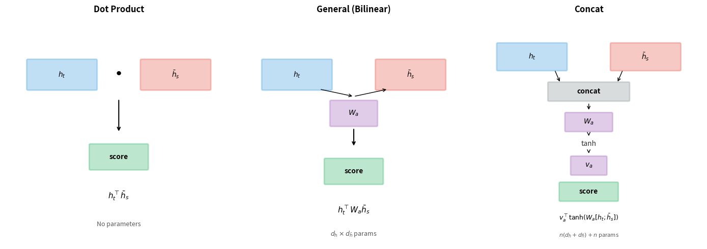
Dot Product Attention
The simplest approach to measuring relevance is to ask: how similar are the decoder and encoder representations? If the encoder has learned to represent "cat" in a particular way, and the decoder has learned to look for that same pattern when generating "chat", then similar representations should yield high scores.
The dot product provides exactly this similarity measure. Given a decoder hidden state and an encoder hidden state , we compute:
where:
- : the decoder hidden state at timestep , encoding what the decoder is "looking for"
- : the encoder hidden state at source position , encoding what that position "contains"
- : the inner product of the two vectors, yielding a scalar score
Why does the dot product capture similarity? Consider what happens geometrically. When two vectors point in the same direction, their dot product is large and positive, indicating high compatibility. When they point in opposite directions, the dot product is large and negative. Orthogonal vectors, sharing no common direction, yield zero.
This geometric interpretation has a powerful implication: the encoder and decoder can learn complementary representations. The encoder learns to place semantically similar words in similar directions in the hidden space. The decoder learns to "query" for specific semantic content by producing hidden states that point toward the relevant encoder representations.
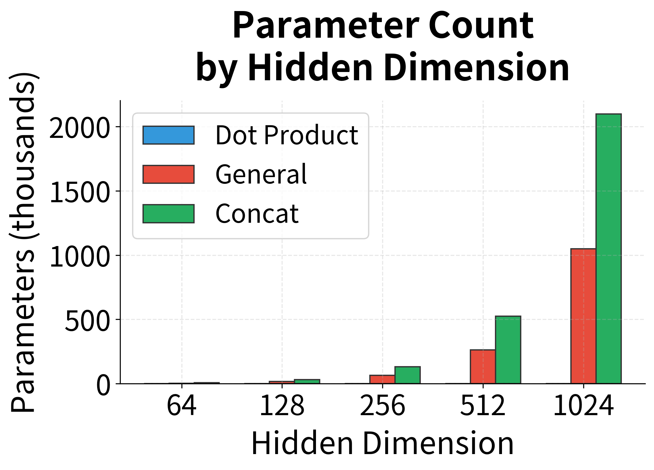
The elegance of dot product attention lies in its simplicity. No learned parameters are needed for the score function itself. All the learning happens in the encoder and decoder, which discover representations where raw similarity is a good proxy for alignment. This makes dot product attention computationally efficient and easy to implement.
However, this simplicity comes with a constraint: the decoder and encoder hidden states must have the same dimensionality. If and , the dot product is well-defined. If they have different dimensions, you cannot compute a dot product directly, which motivates our next score function.
General (Bilinear) Attention
What if the encoder and decoder have different hidden dimensions? Or what if raw similarity isn't the right measure, and we want the model to learn a more nuanced notion of relevance?
The general score function addresses both concerns by introducing a learnable weight matrix that transforms the encoder states before computing similarity:
where:
- : the decoder hidden state at timestep
- : the encoder hidden state at source position
- : a learned weight matrix that projects encoder states into the decoder's space
- : a scalar score computed via matrix-vector multiplication
To understand what does, let's trace through the computation step by step. First, transforms the encoder state into a -dimensional vector. Then takes the dot product with this transformed vector. The matrix effectively learns which aspects of the encoder representation are most relevant for each dimension of the decoder state.
This formulation is called bilinear attention because the score is a bilinear function of the two input vectors: linear in when is fixed, and linear in when is fixed. The weight matrix serves two purposes:
- Dimension matching: When encoder and decoder have different hidden dimensions, bridges the gap by projecting encoder states into the decoder's space
- Learned similarity: Rather than relying on raw vector similarity, the matrix learns what aspects of encoder states are most relevant for alignment, potentially discovering non-obvious relationships
General attention is more expressive than dot product attention but requires additional parameters. For encoder and decoder dimensions of 512, adds parameters. This is modest compared to the total model size but can matter for smaller models or when memory is constrained.
Concat Attention
The most expressive score function takes a fundamentally different approach. Rather than computing a form of similarity between two vectors, it asks: given both the decoder state and an encoder state, what score should a neural network assign?
The concat score function concatenates the two states and passes them through a small neural network:
Let's unpack this formula piece by piece:
-
Concatenation : We stack the decoder and encoder states into a single vector of dimension . This gives the network access to all information from both states.
-
Linear projection : The weight matrix projects the concatenated vector to an intermediate space of dimension . This allows the network to learn arbitrary linear combinations of the input features.
-
Nonlinearity : The hyperbolic tangent activation introduces nonlinearity, enabling the network to learn complex, non-linear relationships between decoder and encoder states.
-
Scalar projection : Finally, the weight vector projects the intermediate representation to a single scalar score.
where:
- : the decoder hidden state at timestep
- : the encoder hidden state at source position
- : the intermediate dimension, a hyperparameter typically set equal to the hidden dimension
This formulation is similar to Bahdanau attention, with one key difference: Bahdanau uses the previous decoder state , while Luong's concat uses the current decoder state . This seemingly small change has significant implications for the overall architecture, which we'll explore in the section on attention placement.
Computational Comparison
The three score functions differ significantly in their computational requirements. Let's analyze them for a sequence of length with hidden dimension :
| Score Function | Time Complexity | Parameters | Notes |
|---|---|---|---|
| Dot Product | 0 | Fastest, requires | |
| General | Matrix multiplication dominates | ||
| Concat | Two-step transformation |
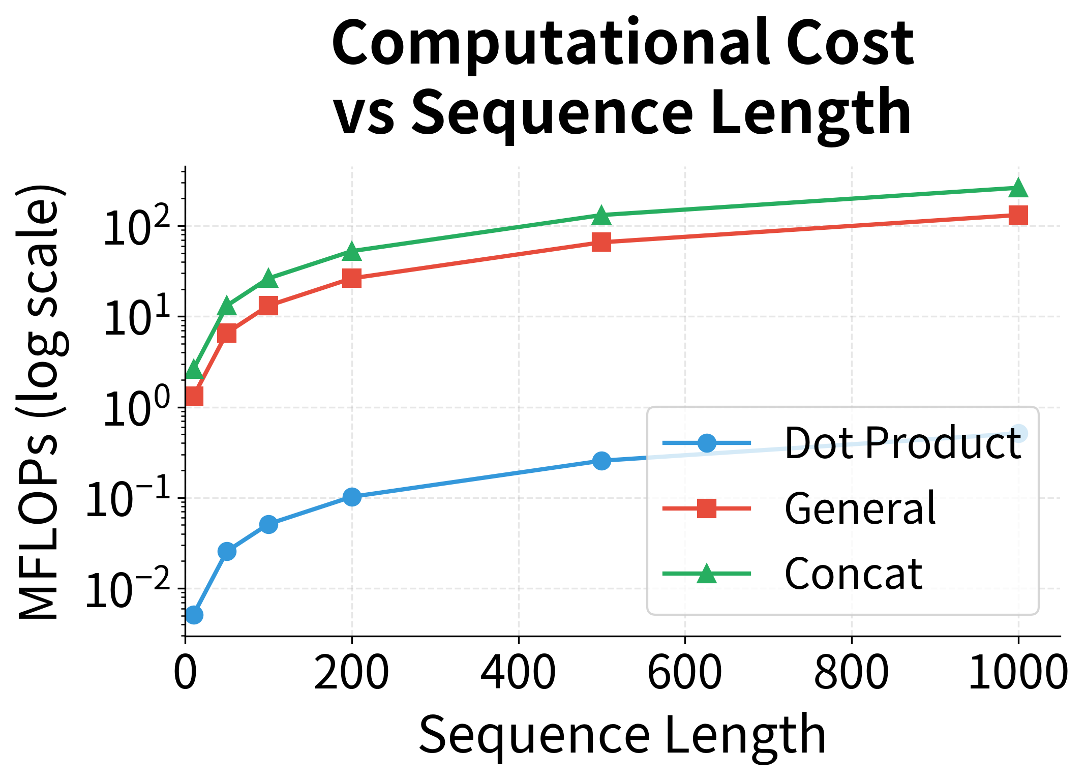
For modern hardware with efficient matrix operations, dot product attention is significantly faster because it can be fully parallelized as a single matrix multiplication across all encoder states simultaneously. This efficiency advantage is why transformers adopt scaled dot-product attention as their core mechanism.
Global vs Local Attention
Beyond score functions, Luong et al. introduced an important architectural distinction: global attention attends to all encoder states, while local attention focuses on a subset of positions around a predicted alignment point.
Global Attention
Global attention is conceptually straightforward. At each decoder timestep , we compute attention weights over all encoder hidden states by applying softmax to the alignment scores:
where:
- : the attention weight for source position when decoding at timestep
- : the alignment score computed using any of the three score functions
- : the total number of encoder positions (source sequence length)
- : the exponential function, ensuring all values are positive
- The denominator normalizes the weights so they sum to 1 across all source positions
The context vector is then computed as the weighted sum of all encoder states:
where:
- : the context vector at decoder timestep
- : the attention weight for position (how much to focus on that position)
- : the encoder hidden state at position
This weighted sum allows the decoder to "focus" on relevant source positions: positions with high attention weights contribute more to the context vector, while positions with low weights contribute less.
Global attention is what we typically mean when we say "attention" without qualification. It allows the model to attend to any position in the source sequence, which is essential for tasks like translation where word order can differ dramatically between languages.
The computational cost of global attention is per decoder step, where is the source sequence length. For most NLP tasks with sequences of hundreds or thousands of tokens, this is manageable. However, for very long sequences (documents, books, genomic data), global attention becomes a bottleneck.
Local Attention
Local attention restricts the attention window to a subset of encoder positions centered around an alignment point . This reduces computation and can also serve as an inductive bias when alignments are expected to be roughly monotonic.
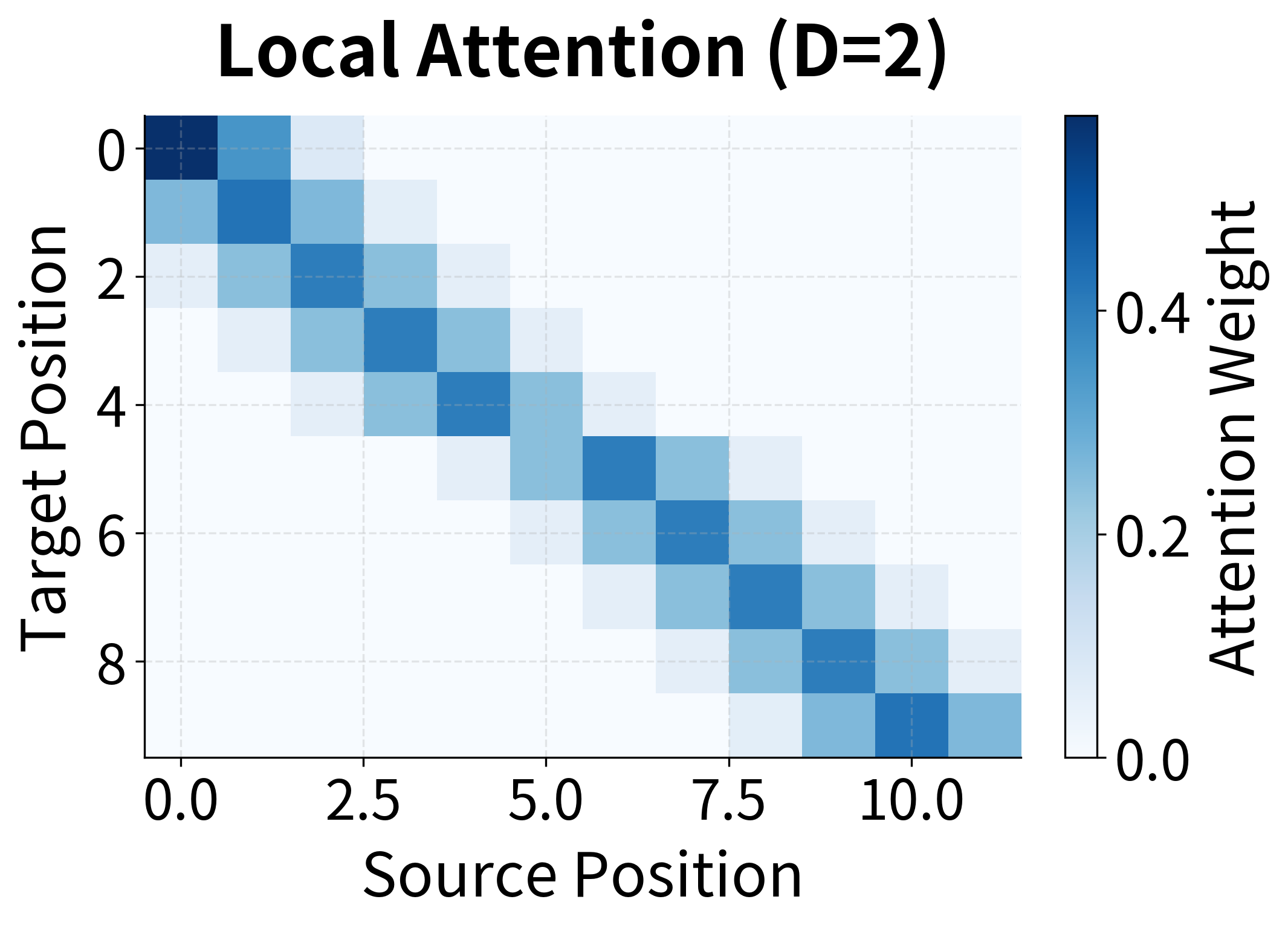
Luong et al. propose two variants for determining the alignment point :
Monotonic alignment (local-m): The alignment point is simply set to , assuming the source and target sequences are roughly aligned. This works well for tasks like speech recognition where the output follows the input order.
Predictive alignment (local-p): The model learns to predict the alignment point using a small neural network:
where:
- : the predicted alignment point (center of the attention window) at decoder timestep
- : the source sequence length
- : the sigmoid function, which outputs a value in
- : a learned weight matrix that transforms the decoder hidden state
- : a learned weight vector that projects to a scalar
- : the current decoder hidden state
The sigmoid ensures the output is between 0 and 1, and multiplying by scales it to a valid source position. This allows the model to learn non-monotonic alignments while still restricting attention to a local window.
Within the window , attention weights are computed normally but multiplied by a Gaussian centered at :
where:
- : the final attention weight for position at decoder timestep
- : the base attention weight from softmax over the local window
- : the source position being attended to
- : the predicted center of the attention window
- : the standard deviation of the Gaussian (controls window sharpness), typically set to
- The exponential term is a Gaussian that peaks at and decays for positions farther from the center
The Gaussian favors positions near the center of the window, providing a soft boundary rather than a hard cutoff. Positions at the edge of the window receive lower weights even if their alignment scores are high.
When to Use Each
The choice between global and local attention depends on your task:
-
Global attention is the default choice for most NLP tasks. Translation, summarization, and question answering all benefit from the ability to attend to any position. The computational overhead is acceptable for typical sequence lengths.
-
Local attention shines when you have prior knowledge about alignment structure. Speech recognition, where phonemes appear in order, is a natural fit. Document-level tasks with very long sequences can also benefit from the reduced computation.
In practice, global attention dominates because modern hardware handles the computation efficiently, and the flexibility to attend anywhere is valuable. Local attention is more of a historical curiosity, though its ideas influenced later work on sparse attention patterns in transformers.
Attention Placement: Input vs Output
A subtle but important difference between Bahdanau and Luong attention is where the attention mechanism fits into the decoder architecture. This choice affects both the information flow and the computational graph.
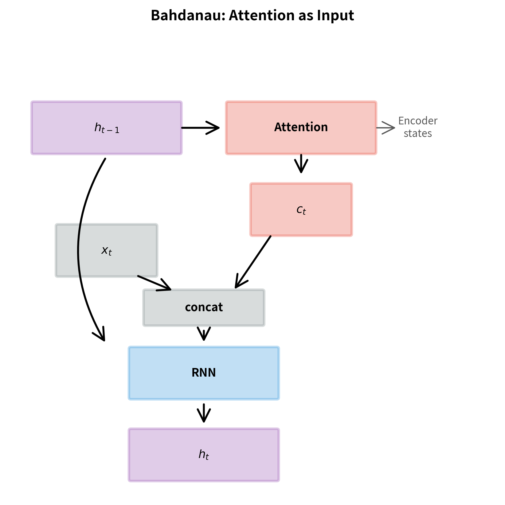
Bahdanau: Attention as Input
In Bahdanau attention, the context vector is computed using the previous decoder hidden state and then concatenated with the input embedding to form the input to the current decoder step. The computation proceeds in three stages:
where:
- : the decoder hidden state from the previous timestep
- : the matrix of all encoder hidden states
- : the context vector computed by attending over encoder states
- : the input embedding at timestep (typically the previous output token)
- : the augmented input formed by concatenating and
- : the new decoder hidden state
The context vector influences the RNN computation directly. This means the decoder can use information about which source positions are relevant when updating its hidden state.
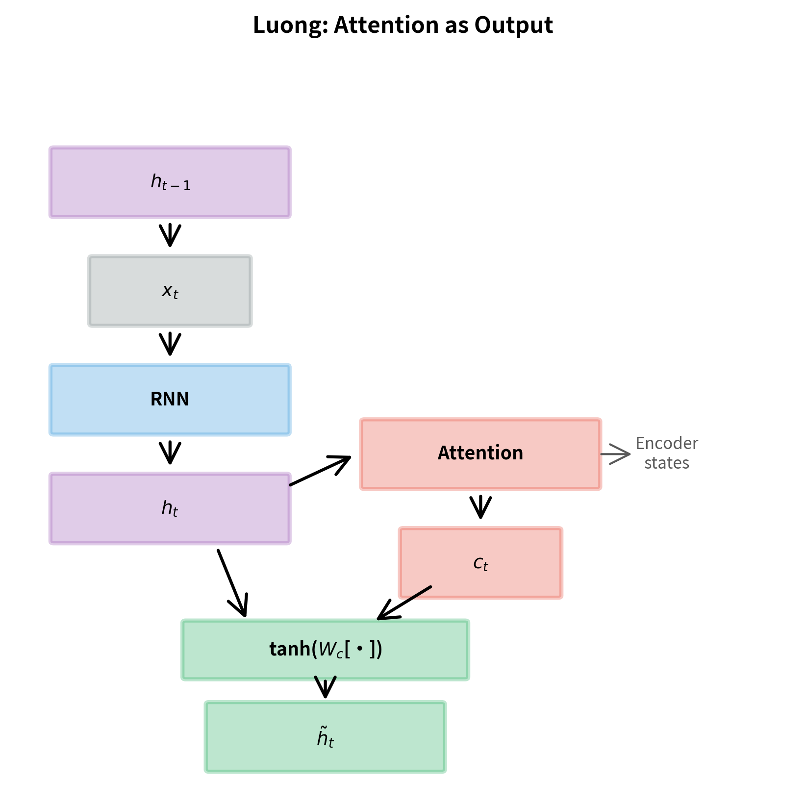
Luong: Attention as Output
In Luong attention, the decoder RNN runs first, producing the current hidden state. Then attention is computed using this new state, and the results are combined. The computation proceeds in three stages:
where:
- : the input embedding at timestep
- : the decoder hidden state from the previous timestep
- : the new decoder hidden state after the RNN step
- : the matrix of all encoder hidden states
- : the context vector computed by attending over encoder states using the current
- : the concatenation of context and hidden state
- : a learned weight matrix that combines context and hidden state
- : the "attentional hidden state" used for prediction
The final output combines the context vector with the decoder state through a learned transformation. This attentional state is then used for prediction, typically by projecting it to vocabulary size and applying softmax.
Implications of Placement
The placement choice has several practical implications:
Information flow: Bahdanau attention allows the context to influence the RNN state update, potentially enabling richer interactions. Luong attention keeps the RNN computation separate, which can be easier to reason about and debug.
Parallelization: Luong attention is slightly more amenable to parallelization during training because the RNN step doesn't depend on the attention computation. However, this advantage is minimal compared to the sequential nature of RNNs themselves.
Empirical performance: Luong et al. found their approach performed comparably or slightly better than Bahdanau attention on machine translation benchmarks. The simpler architecture and faster score functions (especially dot product) made it an attractive choice.
Luong vs Bahdanau: A Complete Comparison
Let's consolidate the differences between these two influential attention mechanisms:
| Aspect | Bahdanau | Luong |
|---|---|---|
| Score function | Additive (concat with tanh) | Dot, general, or concat |
| Decoder state used | Previous () | Current () |
| Attention placement | Before RNN (input) | After RNN (output) |
| Context integration | Concatenated with input | Combined via learned layer |
| Encoder architecture | Bidirectional RNN | Unidirectional (stacked) |
| Parameters | More (additive scoring) | Fewer (dot product option) |
Both mechanisms compute attention weights via softmax and produce a context vector as a weighted sum of encoder states. The differences lie in the details of scoring, timing, and integration.
In practice, the choice between Bahdanau and Luong attention often matters less than other architectural decisions like model size, number of layers, and training procedure. Modern transformer architectures have largely superseded both, but understanding these mechanisms provides essential intuition for how attention works.
Implementation
Let's implement Luong attention in PyTorch. We'll build a complete attention module that supports all three score functions, then integrate it into a sequence-to-sequence decoder.
Attention Module
First, we define the core attention computation. The module takes encoder outputs and a decoder hidden state, computes attention weights, and returns the context vector.
The LuongAttention class implements all three score functions. The constructor accepts the hidden dimension, an optional encoder dimension, and the scoring method. The score method computes alignment scores using dot product, general (bilinear), or concat approaches. The forward method orchestrates the full attention computation: scores, optional masking, softmax normalization, and weighted sum.
Attentional Decoder
Now let's build a decoder that uses Luong attention. The key difference from a standard RNN decoder is the attention step after the RNN and the combination layer that produces the attentional hidden state.
The LuongDecoder class combines an embedding layer, a GRU, the attention module, a combination layer for producing the attentional hidden state, and an output projection. The forward_step method implements a single decoding step: embed, RNN, then attention. This order is the defining characteristic of Luong attention.
Testing the Implementation
Let's verify our implementation works correctly with some example data.
The output has the expected shape for vocabulary logits, and attention weights sum to 1 (ignoring padded positions). The near-zero attention on padded positions confirms our masking works correctly.
Visualizing Attention Patterns
Let's compare the attention patterns produced by different score functions on the same input.

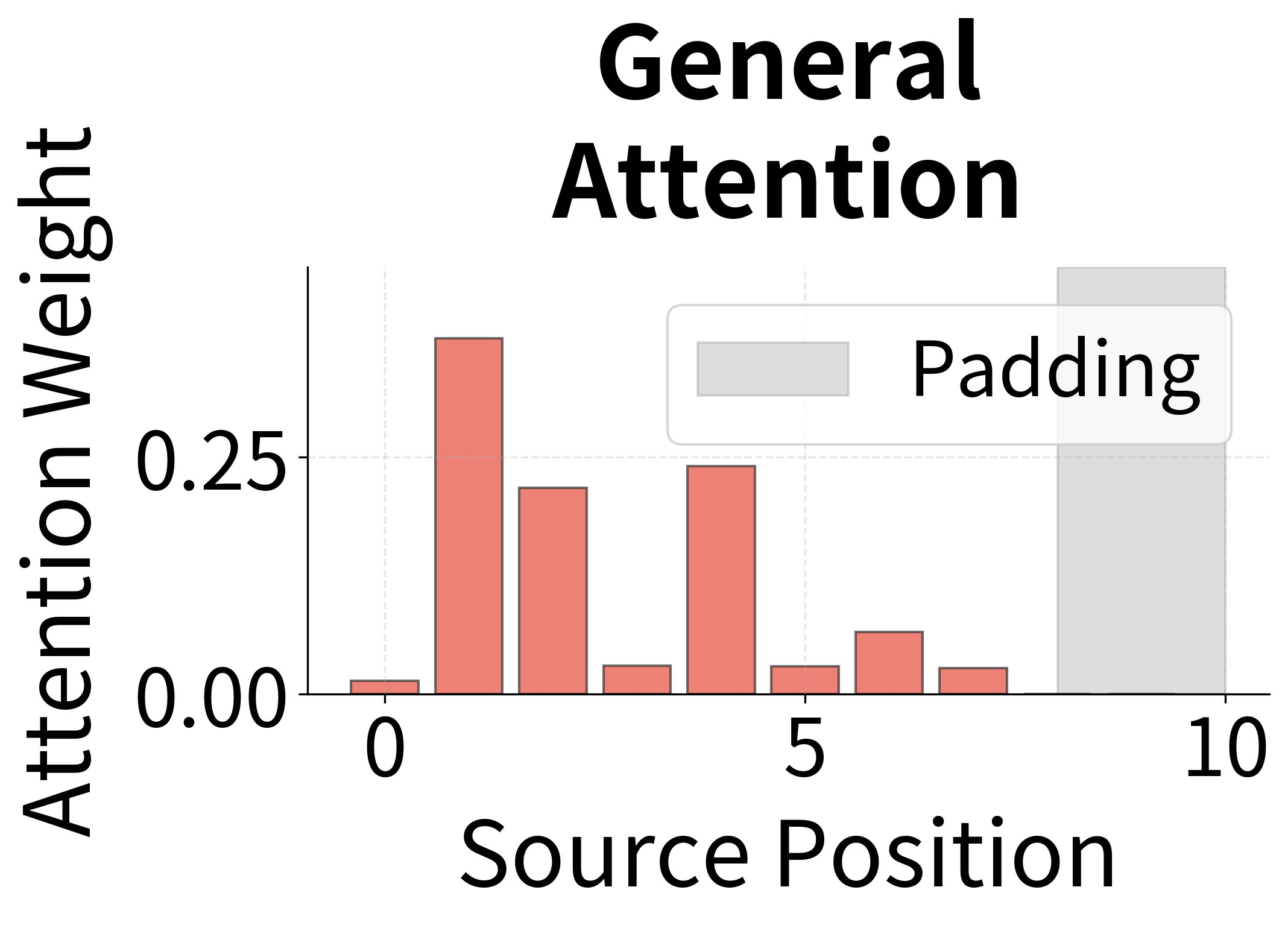
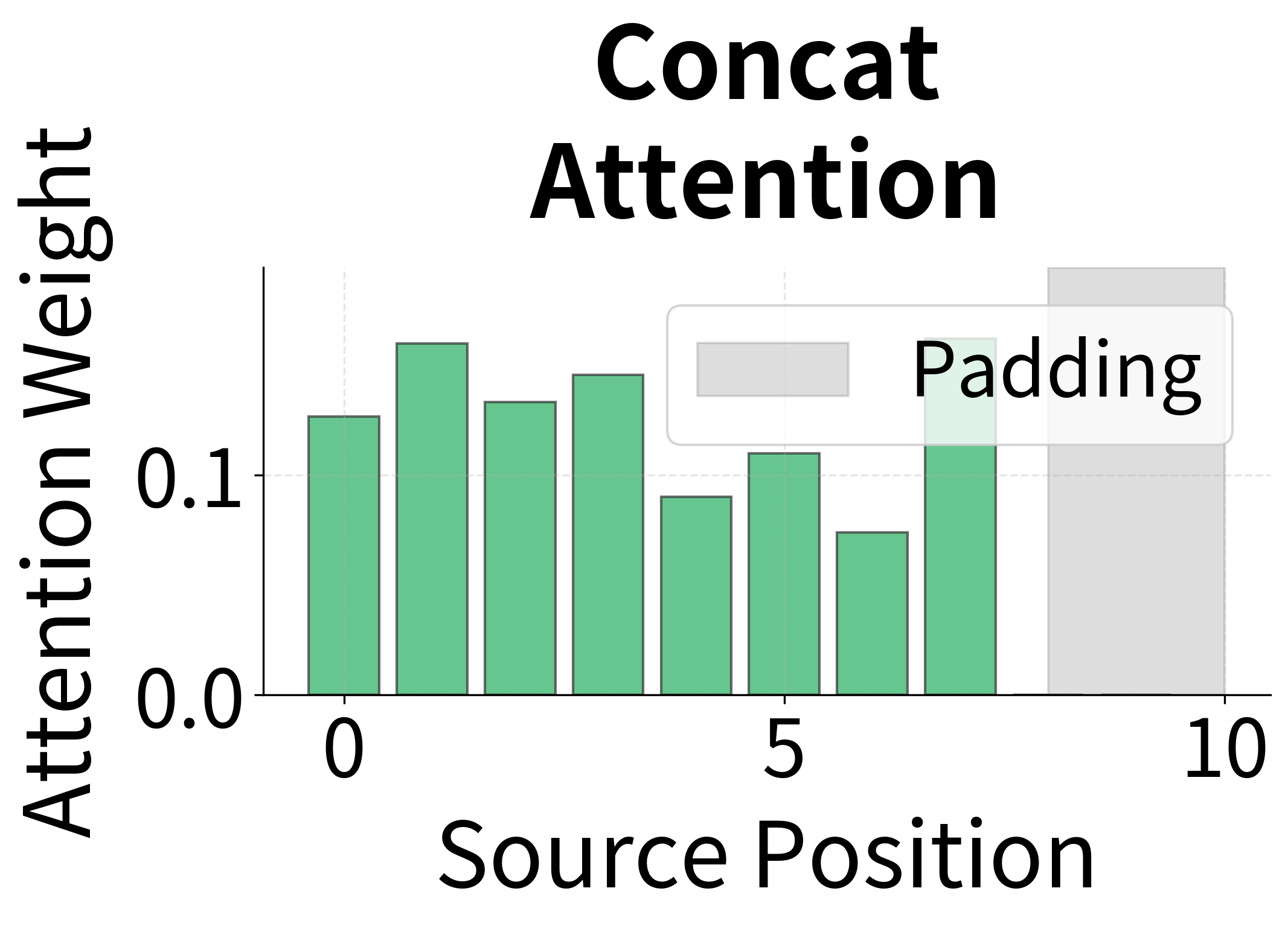
With random weights, the attention patterns are similar across methods. After training, each method would develop distinct patterns based on what it learns about alignment. Dot product attention tends to produce sharper distributions when encoder and decoder representations align well, while concat attention can learn more complex compatibility functions.
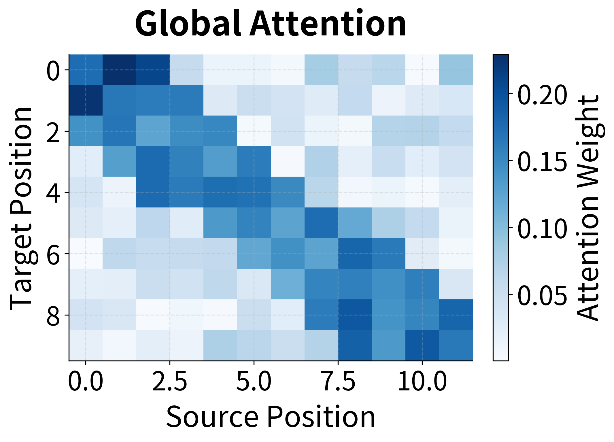
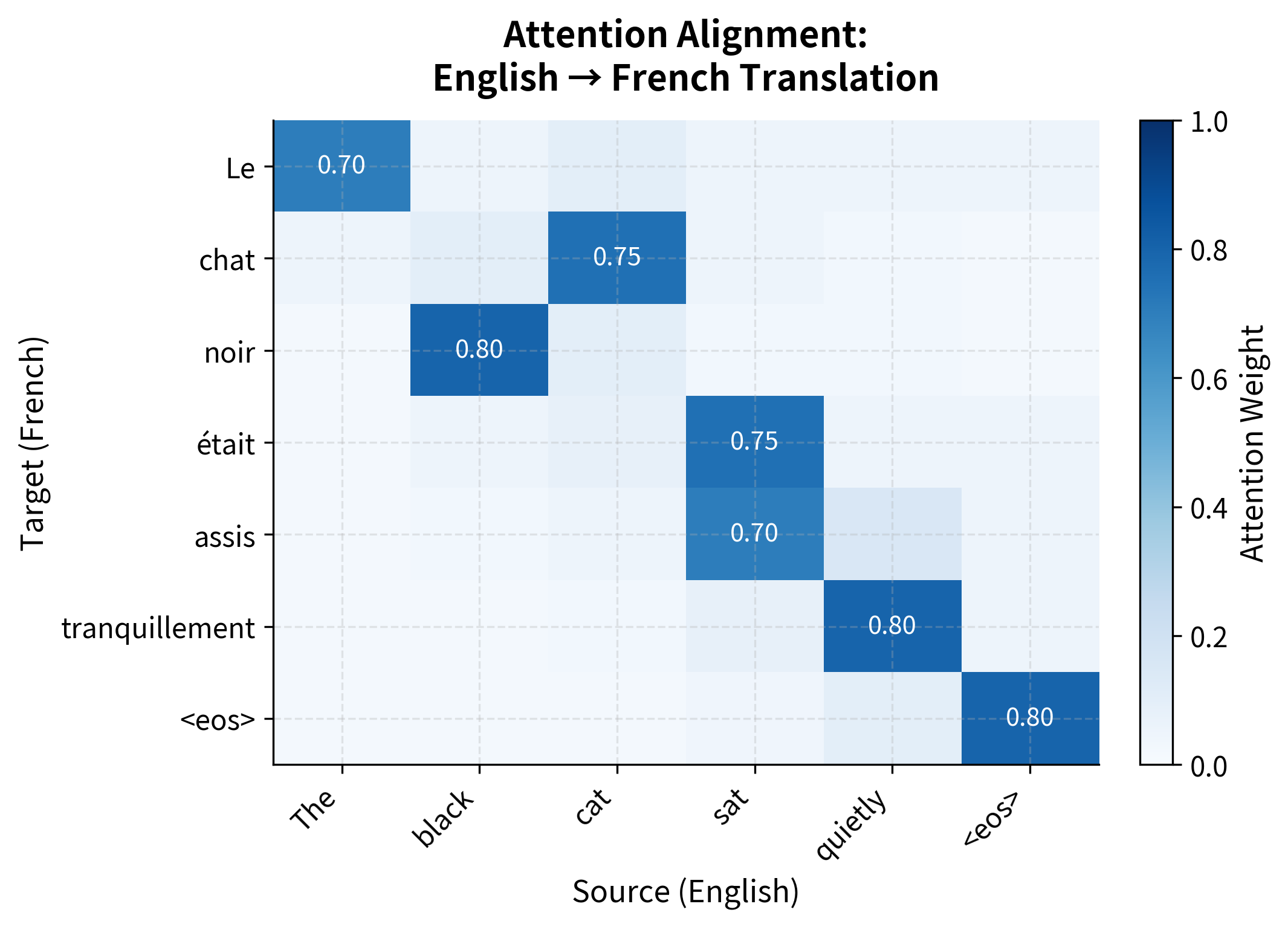
To see what trained attention looks like, let's simulate a full translation with realistic attention patterns. The heatmap below shows attention weights across multiple decoding steps, revealing how the decoder systematically aligns with different source positions.
Worked Example: English-French Alignment
The formulas we've discussed can feel abstract until you see them in action. Let's trace through a complete attention computation for a concrete translation example, following each step from raw hidden states to final attention weights.
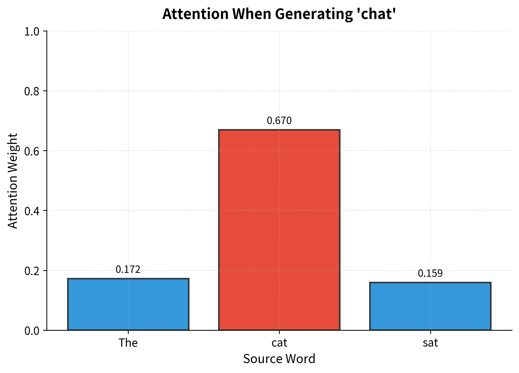
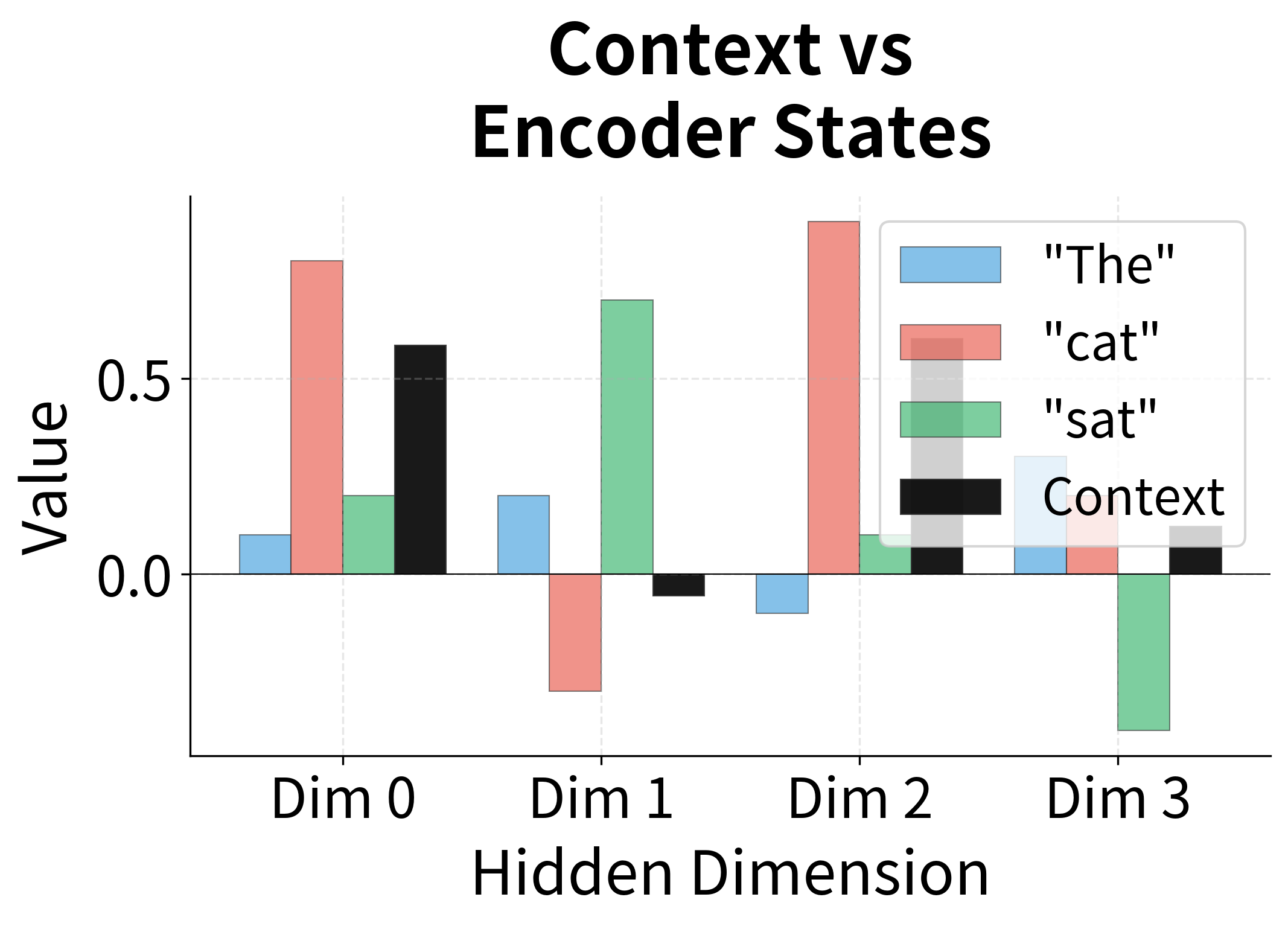
Consider translating the English sentence "The cat sat" to French "Le chat assis". We'll focus on the moment when the decoder is about to generate the second French word "chat". At this point, the decoder needs to figure out which English word to focus on. Intuitively, it should attend to "cat" since that's the word being translated.
Setting Up the Problem
First, let's create simulated encoder hidden states for each English word. In a real model, these would come from running a bidirectional LSTM or transformer encoder over the input. Here, we'll craft vectors that capture the intuition: "cat" and the decoder state for "chat" should be similar, while "The" and "sat" should be less relevant.
The encoder states have shape (1, 3, 4): batch size 1, 3 source words, and 4-dimensional hidden states. The decoder state has shape (1, 4): a single 4-dimensional vector representing what the decoder is "looking for" when generating "chat".
Step 1: Computing Alignment Scores
Now we apply the dot product score function. For each encoder state, we compute its dot product with the decoder state. Remember, the dot product measures how much two vectors point in the same direction.
Step 2: Examining the Results
Let's see what scores each word received and how softmax transforms them into attention weights:
The results reveal exactly what we hoped to see. The decoder state for generating "chat" produces the highest alignment score with "cat" because their vectors point in similar directions. The softmax function then amplifies this difference: "cat" receives about 70% of the attention weight, while "The" and "sat" share the remaining 30%.
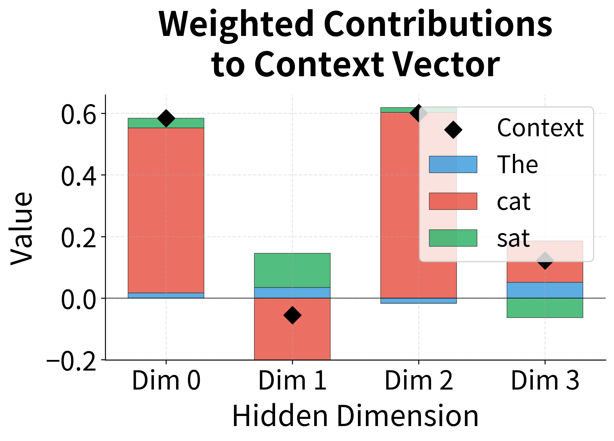
Notice how the context vector ends up being dominated by the "cat" representation. This is attention in action: the decoder has learned to extract the relevant information from the source sequence by focusing on the semantically corresponding word.
The visualization below shows how the context vector is constructed as a weighted blend of the encoder states. Each dimension of the context vector is a weighted sum of that dimension across all encoder states, with the weights determined by attention.
Limitations and Impact
Luong attention addressed several limitations of Bahdanau attention while introducing its own trade-offs. Understanding these helps contextualize attention's evolution toward transformers.
Computational Efficiency
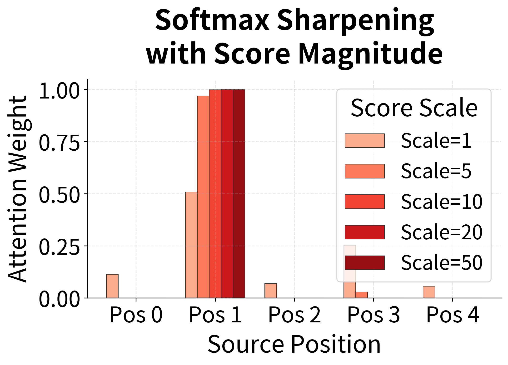
The dot product score function is significantly faster than additive attention, especially for long sequences. With hidden dimension and sequence length , dot product requires operations compared to for additive attention (where is the intermediate dimension). This efficiency gain compounds during training when attention is computed millions of times.
However, dot product attention has a subtle numerical issue: when the hidden dimension is large, dot products can become very large in magnitude. This pushes softmax toward extreme values (near 0 or 1), causing gradient saturation. The transformer architecture addresses this with scaled dot-product attention, dividing by to keep values in a reasonable range.

Expressiveness vs Simplicity
General and concat attention are more expressive than dot product, able to learn arbitrary compatibility functions. But this expressiveness comes at a cost: more parameters, slower computation, and potential overfitting on small datasets. Empirically, the simpler dot product often performs comparably or better, suggesting that the encoder and decoder learn representations where raw similarity is a good proxy for alignment.
This finding influenced the design of transformers, which use dot product attention exclusively. The lesson is that with sufficient model capacity and data, simple mechanisms can match or exceed complex ones.
Sequential Bottleneck
Both Bahdanau and Luong attention still rely on RNNs for the encoder and decoder. This creates a sequential bottleneck: each timestep must wait for the previous one, preventing parallelization. Attention helps by providing direct connections to encoder states, but the fundamental limitation remains.
Transformers eliminate this bottleneck entirely by using self-attention instead of recurrence. Each position can attend to all other positions in parallel, enabling massive speedups on modern hardware. Luong's dot product attention, combined with the key-query-value formulation, became the foundation for this revolution.
Legacy and Influence
Luong attention's most lasting contribution is demonstrating that simple, efficient attention mechanisms work well. The dot product score function, attention after the decoder step, and the idea of multiple attention variants all influenced subsequent research. When Vaswani et al. designed the transformer, they chose scaled dot-product attention, directly building on Luong's work.
The distinction between global and local attention also foreshadowed later work on sparse attention patterns. Transformers face quadratic complexity in sequence length, and researchers have explored various ways to restrict attention to local windows or learned patterns. Luong's local attention was an early exploration of this trade-off between expressiveness and efficiency.
Summary
This chapter explored Luong attention, a family of attention mechanisms that simplified and extended Bahdanau's original formulation.
The key innovations include three score functions for computing alignment:
- Dot product: Parameter-free, efficient, requires matching dimensions
- General: Learned bilinear transformation, handles different dimensions
- Concat: Two-layer network with nonlinearity, most expressive
Luong attention also introduced the distinction between global and local attention. Global attention considers all encoder positions, while local attention focuses on a predicted window. Global attention dominates in practice due to its flexibility and the efficiency of modern hardware.
The architectural placement differs from Bahdanau: Luong computes attention after the RNN step using the current hidden state, then combines the context with the hidden state through a learned transformation. This "attention as output" approach is simpler and slightly more parallelizable.
Perhaps most importantly, Luong's work demonstrated that simple attention mechanisms, particularly dot product attention, can match or exceed more complex alternatives. This insight directly influenced the transformer architecture, which uses scaled dot-product attention as its core mechanism. Understanding Luong attention provides essential context for the self-attention mechanisms we'll explore in the next part of this book.
Key Parameters
When implementing Luong attention, several parameters significantly impact model behavior and performance:
-
Attention method (
method): Chooses between "dot", "general", or "concat" score functions. Dot product is fastest and parameter-free but requires matching encoder/decoder dimensions. General attention adds a learned projection matrix, enabling different dimensions and learned similarity. Concat attention is most expressive but slowest. Start with dot product for most applications. -
Hidden dimension (
hidden_dim): The dimensionality of the decoder hidden state. Larger values (256-512) provide more representational capacity but increase computation. For attention, this determines the space in which similarity is computed. Values of 256-512 work well for most sequence-to-sequence tasks. -
Encoder dimension (
encoder_dim): The dimensionality of encoder hidden states. Can differ fromhidden_dimwhen using general or concat attention. For bidirectional encoders, this is typically2 * hidden_dimsince forward and backward states are concatenated. -
Local attention window (
D): For local attention, controls the half-width of the attention window. Positions outside receive zero attention. Larger windows (D=10-20) provide more flexibility but increase computation. Smaller windows (D=2-5) work well when alignments are expected to be monotonic. -
Dropout (
dropout): Applied to embeddings and the attentional hidden state before output projection. Values of 0.1-0.3 help prevent overfitting, especially important for attention weights which can become overly peaked during training.
Quiz
Ready to test your understanding? Take this quick quiz to reinforce what you've learned about Luong attention mechanisms.

Comments