

Learn how bidirectional RNNs process sequences in both directions to capture past and future context. Covers architecture, LSTMs, implementation, and when to use them.

This article is part of the free-to-read Language AI Handbook
Choose your expertise level to adjust how many terms are explained. Beginners see more tooltips, experts see fewer to maintain reading flow. Hover over underlined terms for instant definitions.
Bidirectional RNNs
Standard RNNs process sequences in one direction: from the first token to the last. At each timestep, the hidden state captures information about everything that came before. But for many tasks, the future matters just as much as the past. When you're trying to understand the meaning of a word in a sentence, you naturally consider both what came before and what comes after.
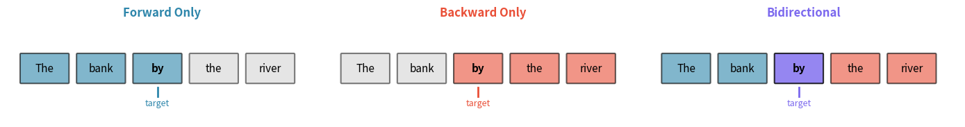
Consider the sentence: "The bank by the river was steep." To understand that "bank" refers to a riverbank rather than a financial institution, you need to see "river" which appears after "bank." A forward-only RNN processing "bank" has no access to this disambiguating context. Bidirectional RNNs solve this problem by running two separate RNNs: one forward through time, one backward. At each position, you get a representation informed by the entire sequence.
The Bidirectional Intuition
Think about how you actually read text. When you encounter an ambiguous word, you don't commit to an interpretation immediately. You keep reading, gathering more context, and then your understanding of earlier words crystallizes. You're implicitly using bidirectional information: past context and future context together inform your understanding of each position.
Bidirectional RNNs formalize this intuition with a simple architectural change. Instead of one RNN, we use two:
- A forward RNN that processes the sequence from position 1 to position , producing hidden states
- A backward RNN that processes the sequence from position to position 1, producing hidden states
At each position , we concatenate these two hidden states to get a combined representation that captures both past and future context:
where:
- : the combined bidirectional hidden state at position
- : the forward hidden state, encoding information from positions
- : the backward hidden state, encoding information from positions
- : the concatenation operator, which stacks two vectors end-to-end
- : the hidden dimension of each directional RNN
The concatenation doubles the dimensionality: if each directional RNN has hidden dimension , the combined representation has dimension .
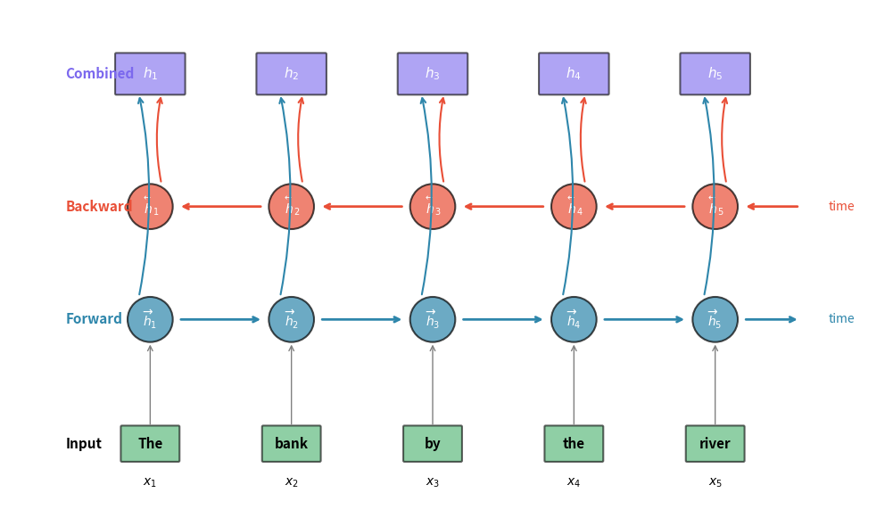
A bidirectional RNN processes a sequence in both directions simultaneously, using a forward RNN and a backward RNN. The hidden states from both directions are combined (typically concatenated) at each position to create representations that capture context from the entire sequence.
Forward and Backward Passes
Now that we understand why bidirectional processing helps, let's formalize how information flows through the architecture. The elegance of bidirectional RNNs lies in their simplicity: we run two completely independent RNNs on the same input, one reading left-to-right and one reading right-to-left. Each builds its own summary of the sequence from its respective direction, and we combine these complementary views at the end.
Consider an input sequence where each is a -dimensional vector, typically a word embedding in NLP or acoustic features in speech recognition. Our goal is to produce a representation at each position that captures context from the entire sequence, not just what came before.
The Forward Pass: Accumulating Left Context
The forward RNN processes the sequence in natural reading order, from position 1 to position . At each step, it faces the same question every recurrent network must answer: how do I combine what I'm seeing right now with everything I've accumulated so far?
The answer is the standard RNN update equation, applied in the forward direction:
Let's unpack each component to understand its role:
- : the input at the current position, the raw information we're processing
- : the previous hidden state, carrying a compressed summary of everything from positions through
- : the input weight matrix, which learns to extract relevant features from the current input
- : the recurrent weight matrix, which learns how to integrate new information with accumulated history
- : a bias vector that shifts the activation
- : an activation function (tanh for vanilla RNNs, or the full gating mechanism for LSTMs and GRUs)
- : the output, a new hidden state that now summarizes positions through
The computation starts with , a zero vector representing "no prior context." As the forward pass proceeds through , each hidden state accumulates progressively more information about the sequence's left context. By the time we reach position , the final forward state has seen the entire sequence, but only from the left-to-right perspective.
The Backward Pass: Accumulating Right Context
The backward RNN performs the mirror-image computation. It starts at the end of the sequence and works its way back to the beginning, building up a summary of what comes after each position:
The structure is identical to the forward pass, but notice the crucial difference in the subscript: the backward hidden state at position depends on , not . This reflects the reversed processing order: the backward RNN has already processed positions before it reaches position .
Each component plays the same role as in the forward pass, but now oriented toward capturing right context:
- : the hidden state from the next position (which the backward RNN has already processed)
- : the backward network's own weight matrices and bias, completely separate from the forward parameters
- : the output, summarizing positions through
The backward pass begins with and proceeds through . By the time it reaches position 1, the state has processed the entire sequence from right to left.
Two Independent Networks with Complementary Views
A crucial architectural point: the forward and backward RNNs are completely separate networks with independent parameters. The forward weights , , share nothing with the backward weights , , . Each network learns its own way of processing the sequence, free to specialize in capturing different types of patterns.
This independence has a direct consequence for model size: a bidirectional RNN has exactly twice the parameters of a unidirectional RNN with the same hidden dimension. If a unidirectional LSTM with hidden size 256 has 1 million parameters, the bidirectional version has 2 million. The doubled capacity is the price we pay for bidirectional context.
Concrete Example: Disambiguating "Bank"
To see how these two passes complement each other, let's trace through our example sentence: "The bank by the river was steep."
When the forward RNN processes "bank" at position 2, its hidden state has only seen "The bank." Based on this limited context, it might tentatively encode "bank" as a financial institution, a reasonable guess given word frequencies. The forward hidden state captures everything to the left, but that's not enough to disambiguate.
When the backward RNN processes "bank" at position 2, the situation is different. It has already processed "was steep," "river," "the," and "by" (in that order). Its hidden state carries this future context, strongly suggesting a geographical feature rather than a financial one. The word "river" appearing later in the sentence is the key disambiguating signal.
By concatenating and , we get a representation that knows both what came before ("The") and what comes after ("by the river was steep"). This combined representation has all the information needed to correctly interpret "bank" as a riverbank.
Hidden State Concatenation
At this point, we have two hidden states at each position: capturing left context and capturing right context. The final step is combining these complementary views into a single representation. This combination operation is where the bidirectional magic happens: we're fusing two partial pictures of the sequence into one complete view.
The Standard Approach: Concatenation
The most common and effective strategy is simple concatenation. We stack the two hidden vectors end-to-end, creating a longer vector that preserves all information from both directions:
where:
- : the combined bidirectional representation at position
- : the forward hidden state, occupying the first elements
- : the backward hidden state, occupying the last elements
Why is concatenation the default choice? It's lossless: no information from either direction is discarded or compressed. The forward and backward components remain distinct, allowing downstream layers to learn how to weight them appropriately for the task at hand. The cost is that the representation doubles in size: if each directional RNN uses hidden dimension 256, the combined output has dimension 512.
Alternative Combination Strategies
While concatenation dominates in practice, other approaches exist. Each makes different trade-offs between information preservation and computational efficiency:
Summation adds the two hidden states element-wise:
This preserves the original dimensionality, which can be convenient when you need to match a specific output size or maintain compatibility with existing architecture. However, summation is lossy. Consider what happens when the forward state has value 0.5 in some dimension and the backward state has -0.5: they cancel out to zero, erasing the information that both directions had strong but opposite signals. The sum can't distinguish "both directions agree on zero" from "both directions disagree strongly."
Element-wise product multiplies corresponding elements:
This captures multiplicative interactions between the directions, which can be powerful when you want to detect patterns that require agreement from both sides. However, it's numerically unstable: if either direction has values near zero, the product collapses regardless of what the other direction says. It also fails when only one direction has relevant information, since a strong signal from one side gets suppressed by a weak signal from the other.
Learned projection concatenates first, then applies a weight matrix:
where is a learned projection matrix. This lets the network learn the optimal way to combine the directions, potentially compressing back to the original dimension () or any other size. The trade-off is additional parameters and computation, plus the risk that the projection might discard useful information during training.
Concatenation remains the standard choice because it's simple, lossless, and numerically stable. The doubled dimensionality is usually acceptable, and downstream layers can learn to weight the forward and backward components appropriately for each task.
Practical Implications of Doubled Dimensions
The doubled output dimension has concrete implications for your network architecture. Any layer that receives the bidirectional output must be sized accordingly:
- A classification layer needs input features instead of
- Attention mechanisms must account for the larger key/value dimensions
- Memory requirements increase proportionally
In PyTorch and similar frameworks, specifying bidirectional=True automatically handles the output dimensionality: the output tensor's last dimension becomes . But when designing custom architectures or debugging dimension mismatches, understanding this doubling is essential.
For sequence-to-sequence models, the decoder typically needs to initialize from the encoder's final state. With a bidirectional encoder, you have two "final" states: from the forward pass (which has seen the whole sequence left-to-right) and from the backward pass (which has seen it right-to-left). Common approaches include concatenating them, summing them, or using a learned projection to combine them into the decoder's initial state.
Bidirectional LSTMs and GRUs
The bidirectional concept we've developed, running two RNNs in opposite directions and concatenating their outputs, is architecture-agnostic. It works identically whether the underlying RNN is a vanilla RNN, an LSTM, or a GRU. In practice, bidirectional LSTMs dominate because they combine bidirectional context with LSTM's ability to capture long-range dependencies. The gating mechanisms that make LSTMs powerful for long sequences work just as well in both directions.
A bidirectional LSTM consists of two independent LSTMs: one processing left-to-right, one processing right-to-left. Each maintains its own hidden state and cell state . The cell state, LSTM's key innovation for preserving information over long distances, operates independently in each direction. Each direction has its own memory pathway, learning to remember and forget different aspects of the sequence.
Forward LSTM: Gated Memory from the Left
At each position , the forward LSTM computes four gate values based on the current input and the previous hidden state. These gates control how information flows into, out of, and through the cell state:
Each gate serves a specific purpose in managing the LSTM's memory:
- : the forget gate, with values between 0 and 1 that decide how much of the previous cell state to retain. A value near 1 means "keep this memory," while near 0 means "discard it."
- : the input gate, which controls how much of the new candidate information to write into memory
- : the output gate, which controls how much of the cell state to expose as the hidden state
- : the candidate cell state, which proposes new values that could be added to memory
- : the collection of forward LSTM weight matrices (one set for each gate)
The cell state update is where LSTM's memory mechanism operates. Old information is selectively forgotten, and new information is selectively added:
where denotes element-wise multiplication. The first term preserves parts of the old cell state that the forget gate allows through. The second term adds parts of the candidate that the input gate admits. This additive structure is what allows LSTMs to maintain information over long distances without the vanishing gradient problems that plague vanilla RNNs.
Finally, the hidden state is computed by filtering the cell state through the output gate:
The tanh squashes the cell state to the range , and the output gate selects which dimensions to expose. This hidden state serves two purposes: it gets passed to the next timestep as input, and it's what we'll eventually concatenate with the backward direction.
Backward LSTM: Gated Memory from the Right
The backward LSTM follows exactly the same gating structure, but with two key differences: it has its own independent set of weights, and it processes in the reverse direction. At position , it uses the hidden state from position , which it has already computed since it started at the end of the sequence:
Notice the subscript pattern: the cell state update uses rather than . The backward LSTM's "previous" state is the state from the next position in the sequence, reflecting its reversed processing order. The backward forget gate decides what to remember from the future (positions through ), while the backward input gate decides what new information from position to add to that future-oriented memory.
Combining the Directions: Hidden States Only
After both passes complete, we have two hidden states at each position: from the forward LSTM and from the backward LSTM. These are concatenated exactly as before:
An important architectural detail: only the hidden states are concatenated. The cell states and remain internal to their respective LSTMs and are never exposed or combined. This makes sense when you consider their roles: the cell state's job is to maintain long-term memory within each direction, serving as a private scratchpad for the LSTM's internal computations. The hidden state is what carries information to the outside world, and that's what we want to combine for downstream tasks.
Implementing Bidirectional RNNs
The mathematics we've developed translates directly into code. Building a bidirectional RNN from scratch reveals the elegant simplicity of the architecture: we literally run two independent RNNs and concatenate their outputs. There's no magic, just two passes over the data in opposite directions.
Let's implement this step by step, starting with the building blocks and working up to a complete bidirectional LSTM.
Building Blocks: Activation Functions and LSTM Cells
Before we can build the bidirectional layer, we need the components that make up each directional LSTM. The sigmoid function squashes values to the range , making it perfect for gates that control information flow (0 = block everything, 1 = let everything through). The tanh function squashes to , used for the candidate cell state and output normalization.
Next, we implement a single LSTM cell. This is the building block that gets replicated at each timestep. The cell takes an input vector and the previous states, computes the four gates, updates the cell state, and produces a new hidden state.
A few implementation details worth noting:
-
Combined weight matrices: Rather than four separate matrix multiplications (one per gate), we concatenate all weights into single large matrices and do one multiplication, then split the result. This is a common optimization that improves computational efficiency.
-
Forget gate bias initialization: The forget gate bias is initialized to 1 rather than 0. This encourages the network to preserve information by default early in training, preventing the common failure mode where the network learns to forget everything before it learns what to remember.
-
Xavier/He initialization: The weight scale
np.sqrt(2.0 / (input_dim + hidden_dim))follows best practices for initializing neural network weights, preventing exploding or vanishing activations at the start of training.
The Bidirectional Layer
Now we build the bidirectional layer itself. The architecture is remarkably simple: create two completely independent LSTM cells (one for each direction) and run them on the same input sequence in opposite orders. The forward LSTM sees positions 0, 1, 2, ..., T-1 in that order; the backward LSTM sees T-1, T-2, ..., 0.
The implementation reveals the core simplicity of bidirectional RNNs:
-
Forward pass: Iterate through positions 0 to in order, updating hidden and cell states at each step. This is identical to a standard LSTM.
-
Backward pass: Iterate in reverse from down to 0. The only tricky part is bookkeeping: we use
backward_states.insert(0, h_bwd)to insert at the front of the list, ensuring thatbackward_states[t]corresponds to position in the original sequence. This alignment is crucial because we need the forward and backward states to match up position-by-position for concatenation. -
Concatenation: Stack the forward and backward states along the feature dimension. At each position , the combined representation has the forward context (from positions 0 through ) in the first half and backward context (from positions through ) in the second half.
Testing the Implementation
Let's verify our implementation produces the expected output shapes and confirm the dimensionality doubling:
The output shapes confirm our implementation is working correctly:
- Input: 5 timesteps × 10 dimensions per timestep
- Forward states: 5 timesteps × 16 hidden units (left context at each position)
- Backward states: 5 timesteps × 16 hidden units (right context at each position)
- Combined output: 5 timesteps × 32 features (full bidirectional context)
The doubling from 16 to 32 is the characteristic signature of bidirectional processing. Every downstream layer that consumes this output must account for this doubled dimensionality.
Visualizing Hidden State Evolution
To build intuition for what the bidirectional LSTM computes, let's visualize how the forward and backward hidden states evolve across the sequence. This reveals the complementary nature of the two directions:
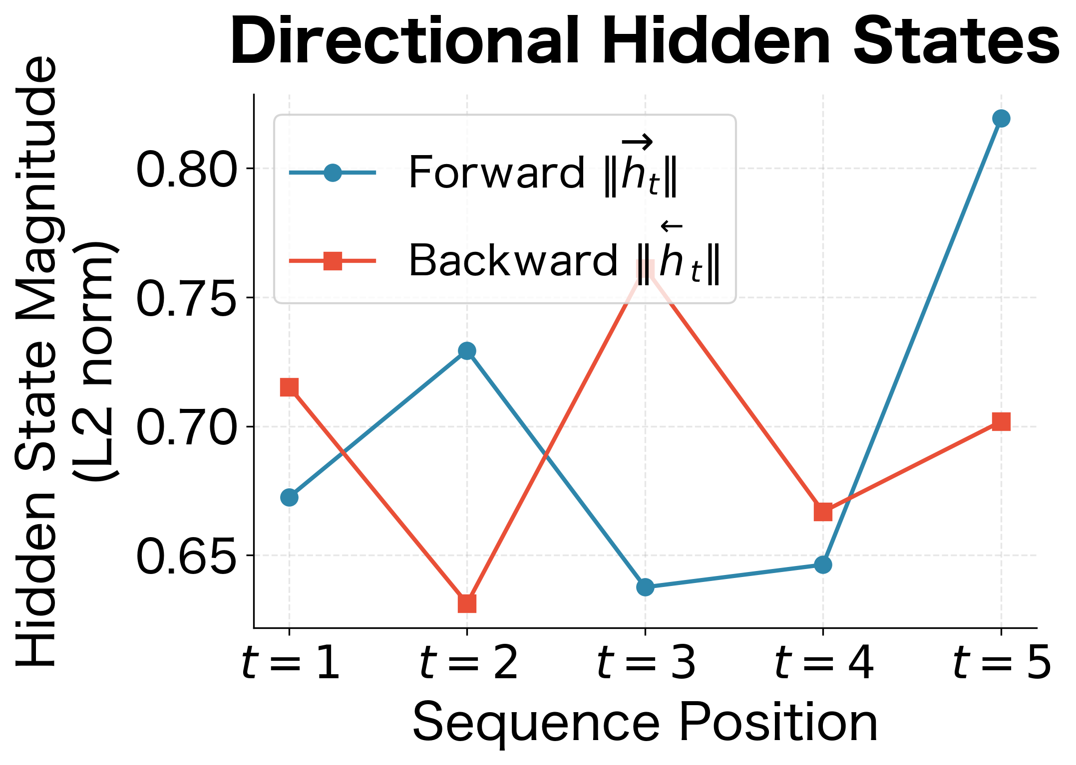
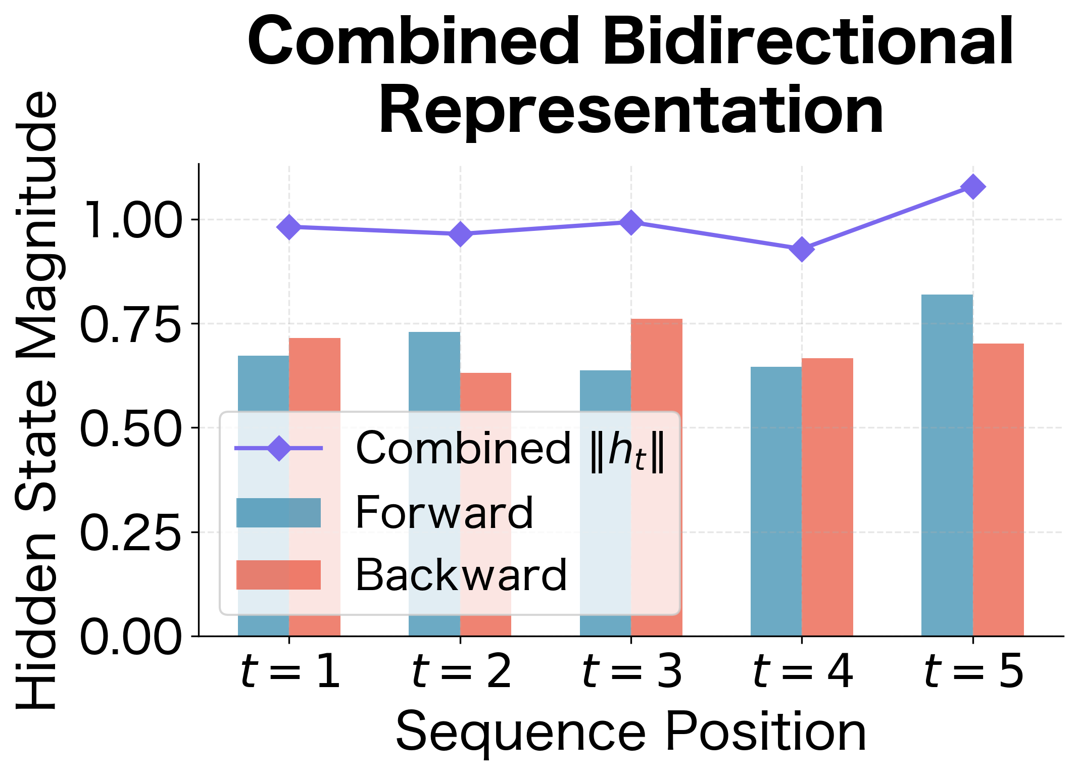
The hidden state magnitudes reveal how each direction builds up its representation over the sequence. With random inputs, the specific patterns depend on the input values, but the key insight is structural: both directions contribute meaningfully at every position. The combined representation (purple diamonds) is always larger than either individual direction because concatenation preserves all information from both passes. We're not losing anything by combining them.
Information Flow: What Each Position "Knows"
The power of bidirectional processing becomes clear when we visualize what information is available at each position. Let's trace how information propagates through the network:
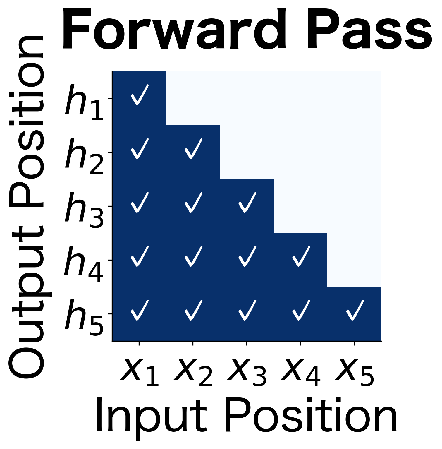
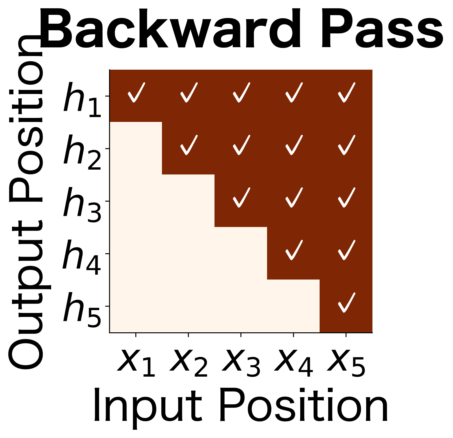
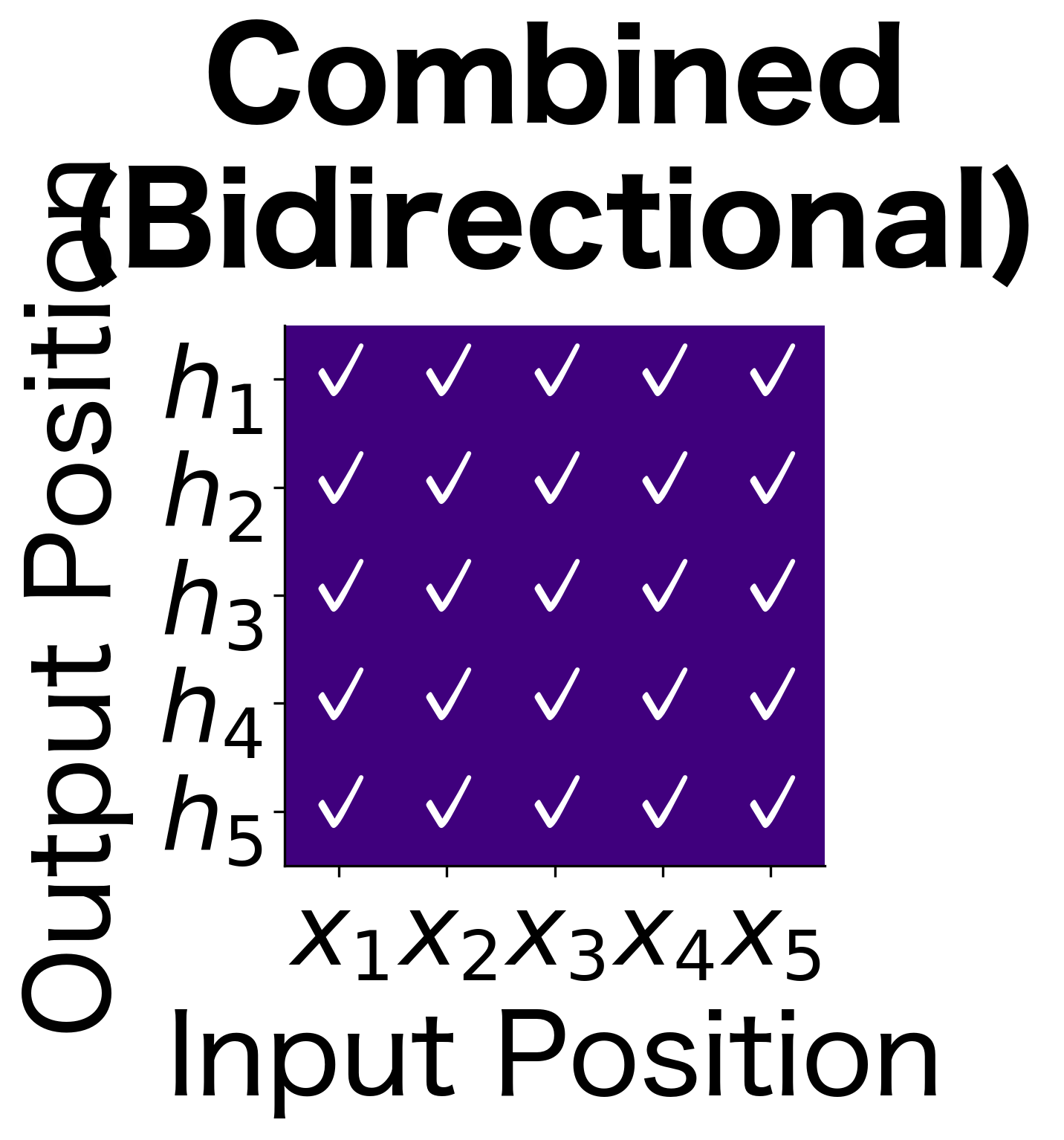
These information flow diagrams illustrate the fundamental difference between unidirectional and bidirectional processing:
- Forward pass (lower triangle): The hidden state at position contains information from inputs 1 through . Early positions have limited context; later positions have seen more of the sequence.
- Backward pass (upper triangle): The hidden state at position contains information from inputs through . The pattern is reversed: early positions have seen more (from the backward perspective).
- Combined (full matrix): Every position has access to the entire sequence. This is the key advantage of bidirectional processing.
Hidden State Activation Patterns
Let's examine the actual hidden state values from our bidirectional LSTM to see what internal representations emerge:
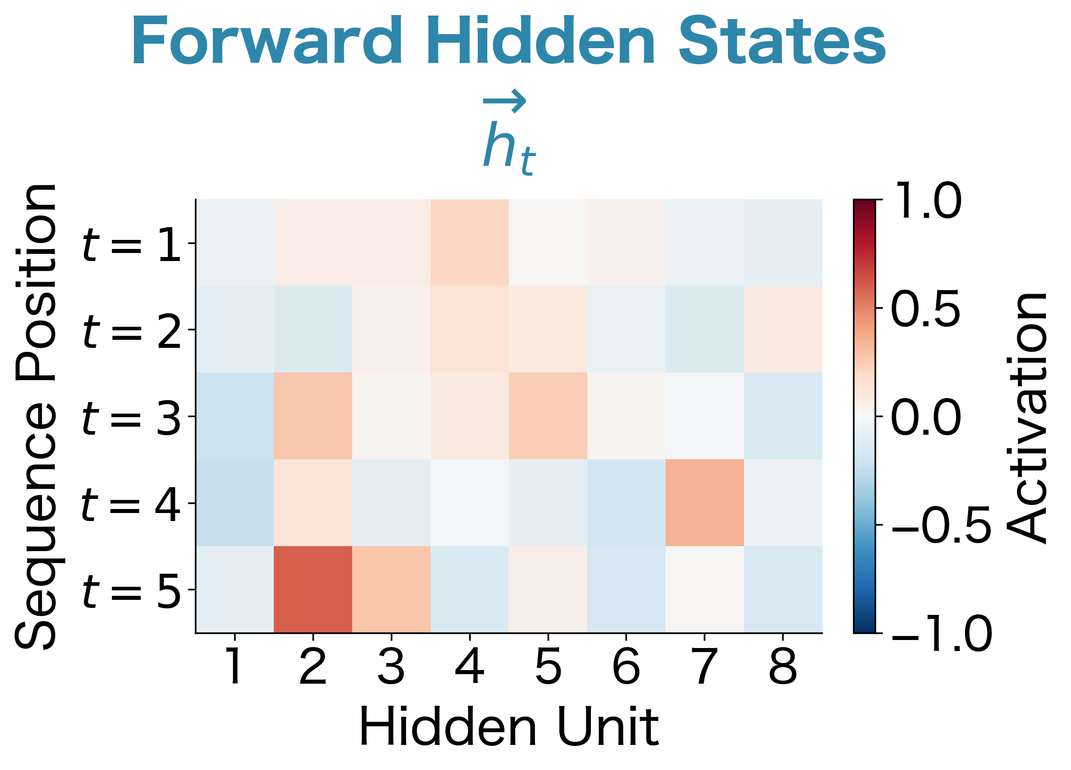
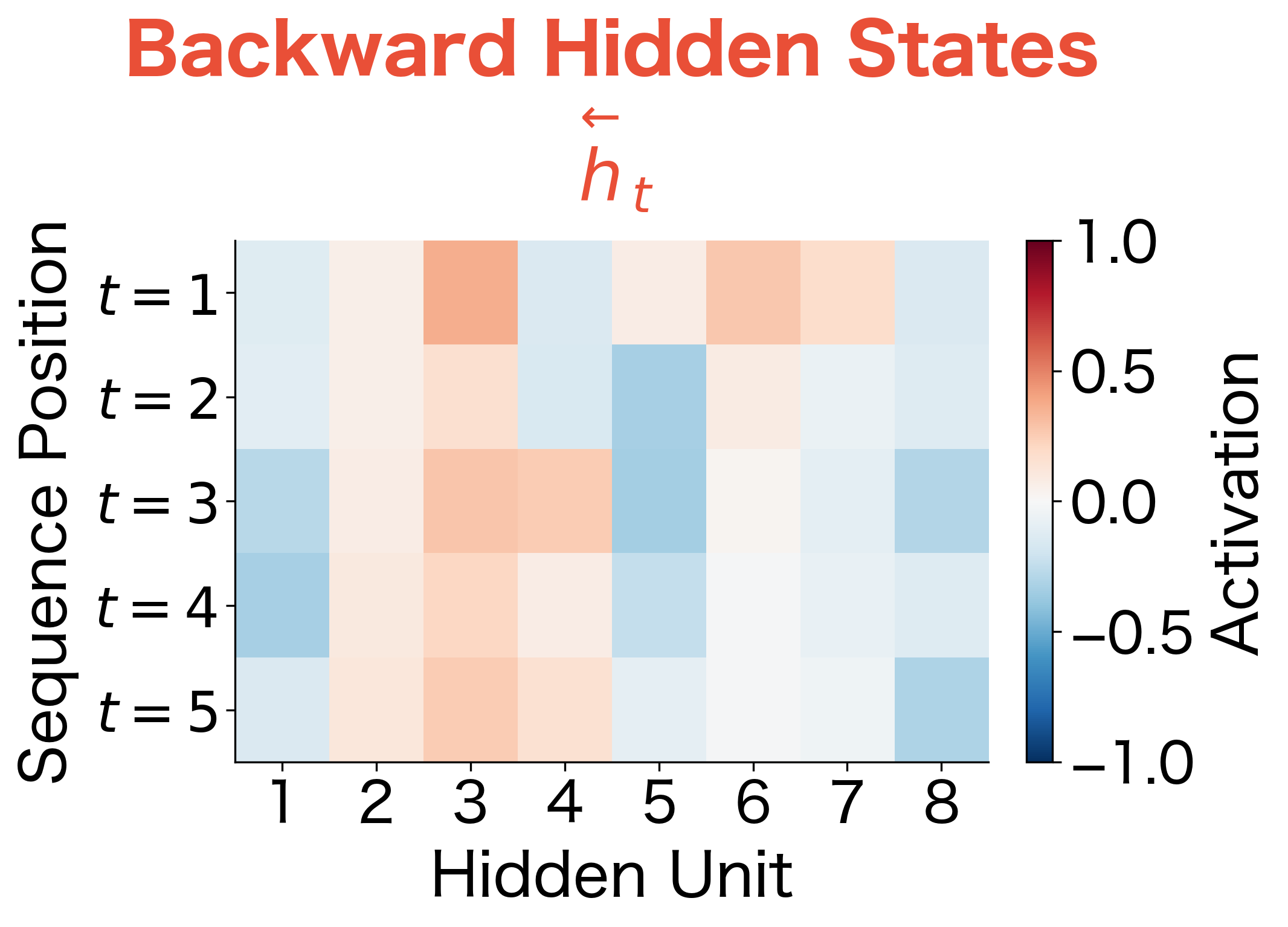
The heatmaps reveal the internal representations computed by each direction. With randomly initialized weights and random inputs, the patterns are essentially arbitrary, but the structure is informative. Notice how different hidden units show different activation patterns across positions, and how the forward and backward passes develop distinct representations.
In a trained model on real data, you would see meaningful patterns emerge: hidden units that activate for specific linguistic features, with forward units capturing left-context patterns (like "the word following 'the' is likely a noun") and backward units capturing right-context patterns (like "the word before 'said' is likely a person"). The bidirectional combination gives downstream layers access to both types of patterns simultaneously.
How Different Are the Two Directions?
A natural question: do the forward and backward passes learn redundant or complementary representations? Let's measure this by computing the correlation between corresponding hidden units in each direction:
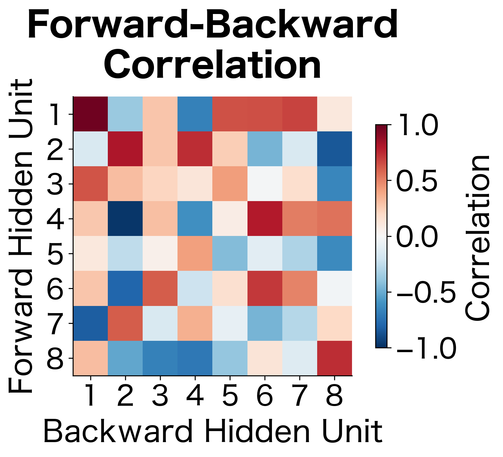
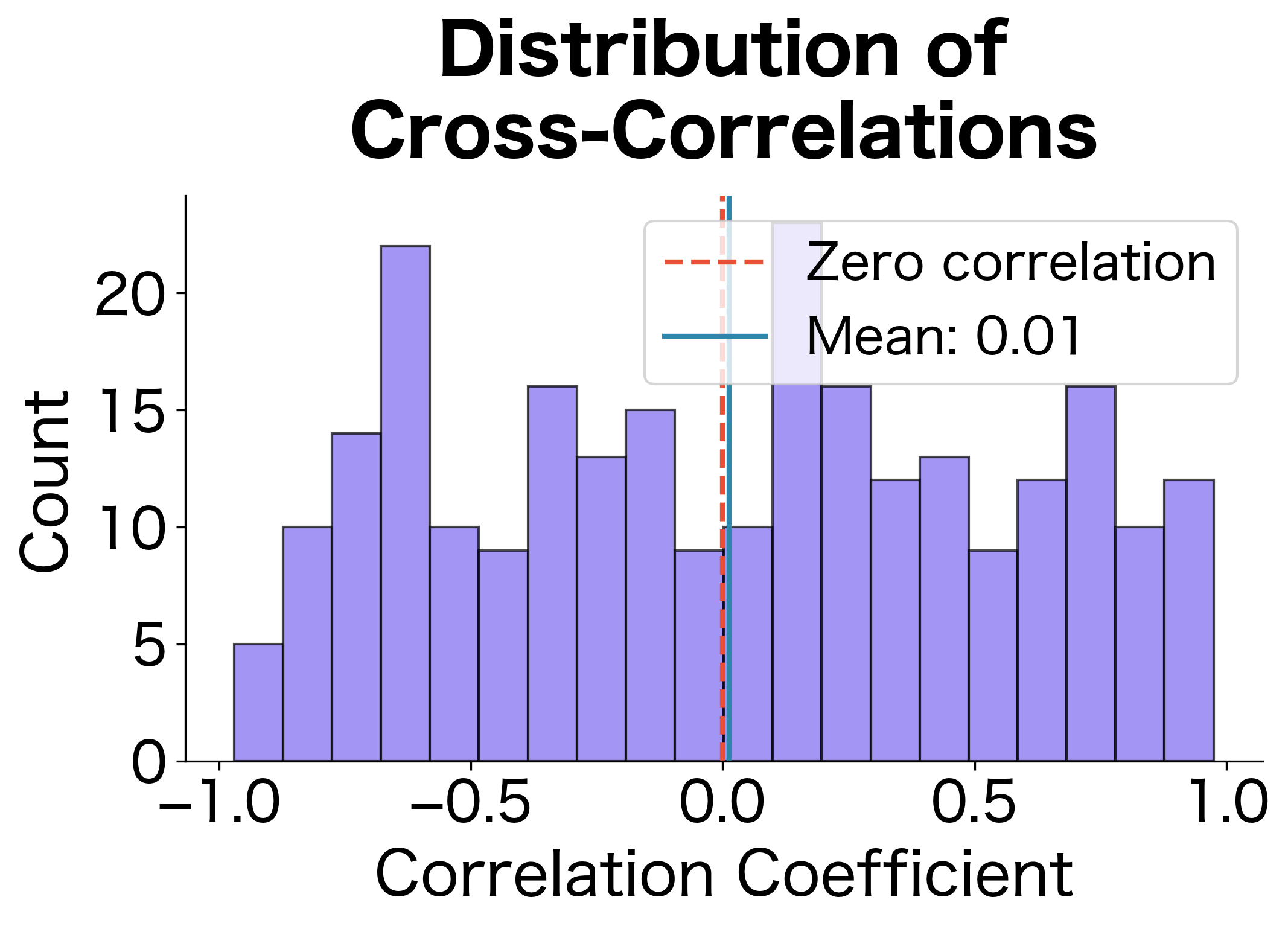
The correlation analysis reveals how independent the two directions are. With random initialization, we expect correlations near zero because the two LSTMs haven't learned to coordinate. In a trained model, you might see some structure emerge: certain forward units might correlate with backward units that capture related (but temporally reversed) patterns. However, the key insight is that low correlation means the directions provide complementary information. If they were highly correlated, concatenation would be wasteful since we'd be duplicating information. The spread of correlations around zero confirms that bidirectional processing genuinely expands the representational capacity.
Bidirectionality for Classification
Bidirectional RNNs excel at classification tasks where you need to make a decision based on the entire sequence. Sentiment analysis, named entity recognition, and part-of-speech tagging all benefit from bidirectional context.
Sequence Classification
For classifying an entire sequence (e.g., sentiment of a review), you typically use the final hidden states from both directions:
The classifier processes an 8-token sequence and produces logits for each class. The softmax converts these to probabilities that sum to 1. With randomly initialized weights, the predictions are essentially random, but the architecture correctly combines bidirectional context: the final forward state captures information from all 8 tokens read left-to-right, while the final backward state captures information from all 8 tokens read right-to-left.
Token-Level Classification
For tasks like named entity recognition where you classify each token, you use the combined representation at each position:
The tagger produces a 5-dimensional logit vector at each of the 6 positions, one score per possible tag. The argmax selects the highest-scoring tag for each token. With random weights, the predictions are meaningless, but the key point is that each token's prediction uses the full bidirectional context: the combined hidden state at position incorporates information from all tokens before and after it.
The bidirectional context is particularly valuable for NER because entity boundaries often depend on both preceding and following words. "Bank of America" needs the following "of America" to recognize "Bank" as part of an organization name.
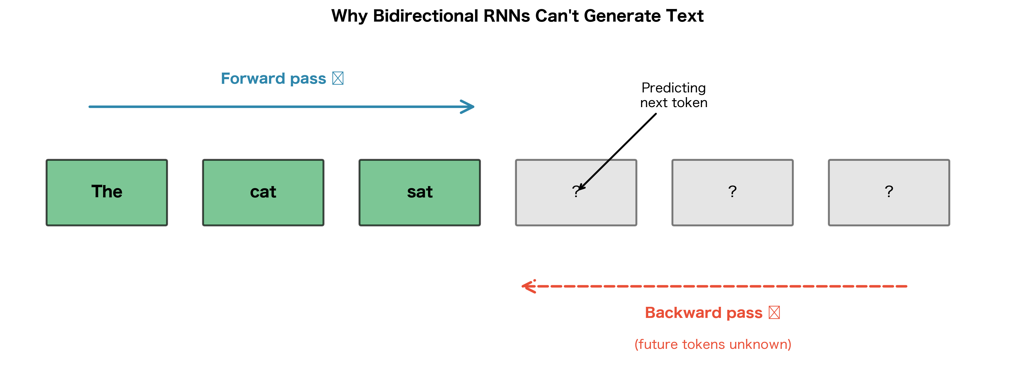
Limitations for Generation
Bidirectional RNNs have a fundamental limitation: they cannot be used for autoregressive generation. When generating text one token at a time, you don't have access to future tokens because they haven't been generated yet.
Consider a language model trying to predict the next word. At position , an autoregressive model can only use information from positions . The backward pass of a bidirectional RNN would require information from positions , which don't exist during generation.
This limitation means bidirectional RNNs are used for:
- Encoding in sequence-to-sequence models (the encoder sees the full input)
- Classification tasks where the full sequence is available
- Feature extraction for downstream tasks
But not for:
- Language modeling (predicting next tokens)
- Text generation (writing stories, completing sentences)
- Decoders in seq2seq models (which generate one token at a time)
PyTorch Implementation
PyTorch provides built-in support for bidirectional RNNs. Let's see how to use it and verify our understanding:
PyTorch's bidirectional LSTM automatically handles the forward and backward passes and concatenates the results. The output shape confirms the doubled dimensionality: 32 features instead of 16. The final hidden state tensor has shape (2, 1, 16), where the first dimension indexes direction (0 = forward, 1 = backward), the second is batch size, and the third is hidden dimension. This matches our from-scratch implementation.
Extracting Directional States
To access the forward and backward components separately:
Slicing the output tensor along the feature dimension separates the forward and backward components. Each has shape (1, 5, 16), corresponding to batch size, sequence length, and hidden dimension. The final hidden states for each direction have shape (1, 16), representing the last state computed by each directional LSTM. These can be concatenated for sequence classification or used separately depending on your task.
Visualizing the Concatenated Output Structure
To make the structure of bidirectional output concrete, let's visualize how the forward and backward components are arranged in the concatenated tensor:
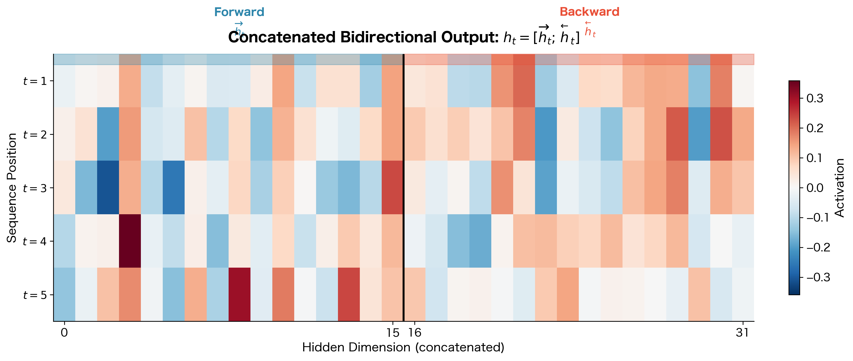
The visualization makes the concatenation structure explicit: at each position , the output vector has dimensions. The first dimensions (indices 0 to ) contain the forward hidden state , encoding left context. The second dimensions (indices to ) contain the backward hidden state , encoding right context. When you slice output[:, :, :hidden_dim], you get the forward component; output[:, :, hidden_dim:] gives you the backward component.
Comparing Unidirectional and Bidirectional Performance
Let's design an experiment that demonstrates the advantage of bidirectional processing. We'll create a task where context from both directions is necessary for correct classification.
The Bracket Matching Task
We'll create sequences with matching brackets where the model must classify whether each position is inside or outside a bracket pair. This requires seeing both the opening bracket (past) and closing bracket (future).
Now let's train both unidirectional and bidirectional models:
The bidirectional model achieves near-perfect accuracy because it can see both the opening and closing brackets when classifying each position. The unidirectional model struggles because when it processes a position, it doesn't know if a closing bracket will appear later. This task is specifically designed to require future context: determining whether a position is inside brackets needs information about both the opening bracket (past) and closing bracket (future).
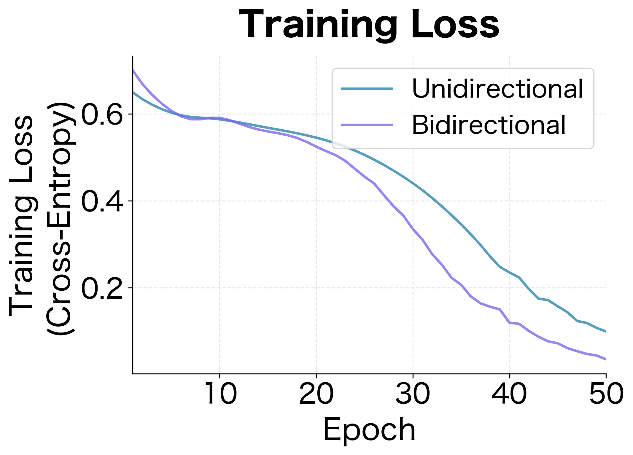
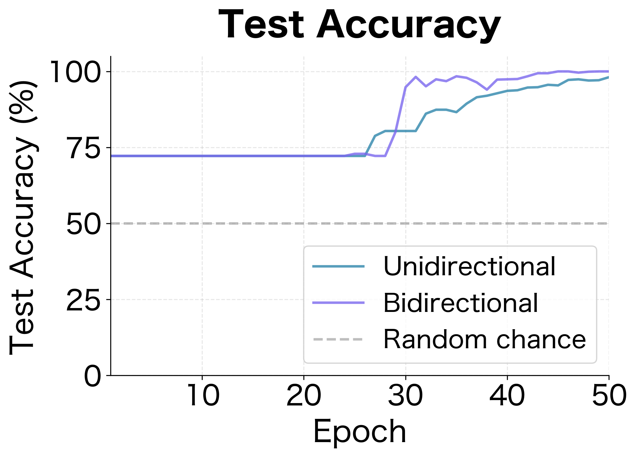
The learning curves reveal the dynamics of training. The bidirectional model not only achieves higher final accuracy but also learns faster, reaching good performance within the first few epochs. The unidirectional model's loss decreases but plateaus at a higher value, reflecting its fundamental inability to solve the task perfectly without future context.
Where Does the Unidirectional Model Fail?
To understand why the unidirectional model struggles, let's analyze accuracy by position within the sequence. The bracket matching task has a specific structure: positions before the opening bracket should be labeled "outside," positions between brackets should be "inside," and positions after the closing bracket should be "outside."
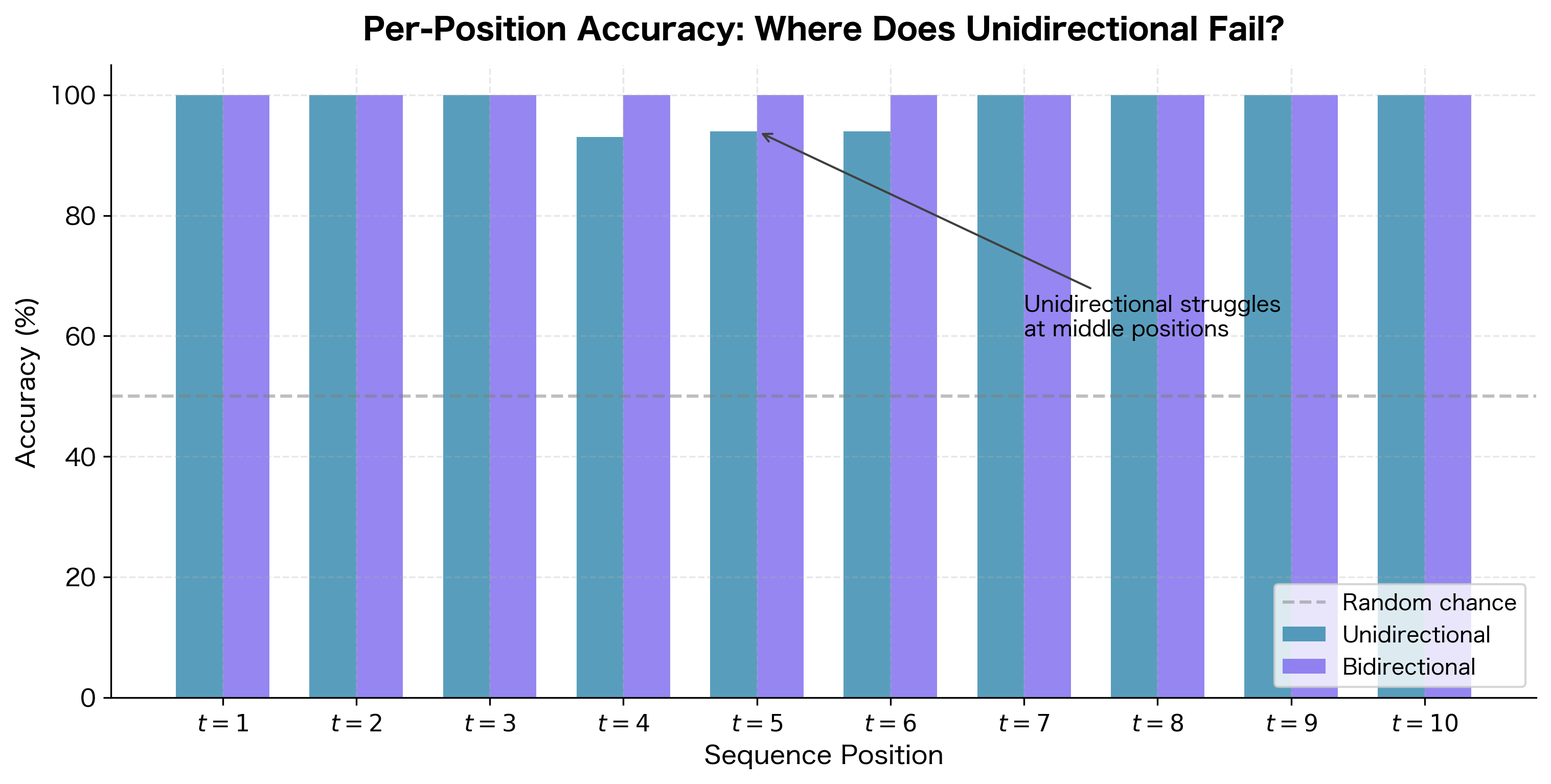
The per-position analysis reveals the fundamental limitation of unidirectional processing. Early positions (near the start of the sequence) tend to have higher accuracy because they're more likely to be before any bracket, so the model can correctly predict "outside" without needing future context. However, middle positions are problematic: the unidirectional model has seen the opening bracket but doesn't know if or when a closing bracket will appear. It must guess whether the current position is inside or outside brackets based only on past context.
The bidirectional model maintains high accuracy at all positions because it has access to the full sequence. When classifying position 5, it knows both that an opening bracket appeared at position 2 and that a closing bracket appears at position 7. This complete picture enables correct classification regardless of position.
Practical Considerations
When deciding whether to use bidirectional RNNs, consider these factors:
When to Use Bidirectional RNNs
Bidirectional architectures are well-suited for tasks where:
- The entire input sequence is available before making predictions
- Context from both directions improves understanding (most NLP classification tasks)
- You're building an encoder that will feed into a decoder
- Token-level predictions depend on surrounding context (NER, POS tagging)
When to Avoid Bidirectional RNNs
Stick with unidirectional architectures when:
- You need to generate sequences autoregressively
- You're processing streaming data where future inputs aren't available
- Latency is critical and you can't wait for the full sequence
- You're building a decoder in a seq2seq model
Parameter and Computation Cost
Bidirectional RNNs double both parameters and computation compared to unidirectional versions with the same hidden size. If you need a bidirectional model with the same total capacity as a unidirectional one, use half the hidden size in each direction.
The parameter counts reveal the cost of bidirectionality:
| Configuration | Hidden Size | Parameters | Output Dim | Notes |
|---|---|---|---|---|
| Unidirectional | 256 | 366,592 | 256 | Baseline |
| Bidirectional | 256 | 733,184 | 512 | 2× parameters |
| Bidirectional | 128 | 188,416 | 256 | Similar to unidirectional |
A bidirectional LSTM with hidden size 256 has exactly twice the parameters of a unidirectional one, since it maintains two complete sets of weights. If you need to match parameter budgets, using hidden size 128 in each direction gives you bidirectional context with roughly the same total parameters as a unidirectional model with hidden size 256. The trade-off is that each direction has less capacity, but the combined representation still benefits from seeing the full sequence.
Limitations and Impact
Bidirectional RNNs solved a critical limitation of unidirectional sequence models: the inability to incorporate future context. This architectural innovation had significant impact across NLP, enabling substantial improvements on tasks from named entity recognition to machine translation encoders.
The most significant practical limitation remains the incompatibility with autoregressive generation. You cannot use bidirectional models for language modeling, text generation, or any task requiring sequential token-by-token output. This fundamental constraint means that even as bidirectional encoders became standard, unidirectional decoders remained necessary for generation tasks.
Computational cost presents another consideration. Processing sequences in both directions doubles the computation and memory requirements compared to unidirectional models. For very long sequences or resource-constrained environments, this overhead may be prohibitive. The sequential nature of RNNs compounds this issue: you cannot parallelize across time steps, so processing time scales linearly with sequence length regardless of available hardware.
Despite these constraints, bidirectional RNNs became a foundational component of modern NLP. The ELMo model, which achieved state-of-the-art results across many benchmarks in 2018, used deep bidirectional LSTMs. BERT and subsequent transformer models adopted the bidirectional principle, though they achieved bidirectionality through attention mechanisms rather than separate forward and backward passes. The insight that both past and future context matter for understanding language proved more durable than any specific architectural implementation.
Summary
Bidirectional RNNs process sequences in both directions simultaneously, combining forward and backward hidden states to create representations informed by the entire sequence context.
The key architectural components are:
- A forward RNN processing from position 1 to , producing states
- A backward RNN processing from position to 1, producing states
- Concatenation at each position:
This architecture excels at classification tasks where full sequence context improves predictions. Named entity recognition, sentiment analysis, and part-of-speech tagging all benefit from bidirectional processing. The encoder in sequence-to-sequence models typically uses bidirectional RNNs to capture complete input context.
The fundamental limitation is incompatibility with autoregressive generation. Since future tokens don't exist during generation, the backward pass cannot be computed. Language models, text generators, and decoders must use unidirectional architectures.
Bidirectional RNNs double both parameters and computation compared to unidirectional versions. When computational budget is fixed, using half the hidden size in each direction maintains similar total capacity while gaining bidirectional context.
Key Parameters
When working with bidirectional RNNs in PyTorch (nn.LSTM, nn.GRU, nn.RNN), the following parameters are most relevant:
-
bidirectional: Set to
Trueto enable bidirectional processing. This doubles the output dimension and the number of parameters. -
hidden_size: The hidden dimension for each direction. With
bidirectional=True, the output dimension becomes2 * hidden_size. -
num_layers: Number of stacked RNN layers. Each layer can be bidirectional independently, though typically all layers share the same directionality.
-
batch_first: When
True, input and output tensors have shape(batch, seq, features). The bidirectional output features are concatenated along the last dimension. -
dropout: Applied between layers (when
num_layers > 1). Does not affect bidirectionality but helps regularize deeper bidirectional stacks.
The output tensor shape is (batch, seq_len, num_directions * hidden_size) where num_directions is 2 for bidirectional models. The final hidden state has shape (num_layers * num_directions, batch, hidden_size), with forward and backward states interleaved by layer.
Quiz
Ready to test your understanding? Take this quick quiz to reinforce what you've learned about bidirectional RNNs and how they capture context from both directions.

Comments