

Learn how LSTMs solve the vanishing gradient problem through the cell state gradient highway. Includes derivations, visualizations, and PyTorch implementations.

This article is part of the free-to-read Language AI Handbook
Choose your expertise level to adjust how many terms are explained. Beginners see more tooltips, experts see fewer to maintain reading flow. Hover over underlined terms for instant definitions.
LSTM Gradient Flow
In the previous chapters, we saw how vanilla RNNs suffer from vanishing gradients and how LSTMs introduce gates to control information flow. But we haven't yet examined the mathematical reason why LSTMs solve the vanishing gradient problem. The answer lies in how gradients flow through the cell state, a mechanism sometimes called the constant error carousel.
This chapter analyzes gradient flow in LSTMs from first principles. We'll derive the gradient equations, show why the cell state acts as a "gradient highway," compare gradient behavior between vanilla RNNs and LSTMs, and explore when LSTMs still need gradient clipping. We'll also examine peephole connections, a variant that allows gates to directly observe the cell state.
The Constant Error Carousel
The term "constant error carousel" comes from Hochreiter and Schmidhuber's original 1997 paper. It describes the key insight that makes LSTMs work: the cell state can carry information (and gradients) across many timesteps without the multiplicative decay that plagues vanilla RNNs.
Recall the cell state update equation from the previous chapter:
where:
- : the cell state at timestep
- : the forget gate activation (values between 0 and 1)
- : the cell state from the previous timestep
- : the input gate activation
- : the candidate cell state
- : element-wise multiplication
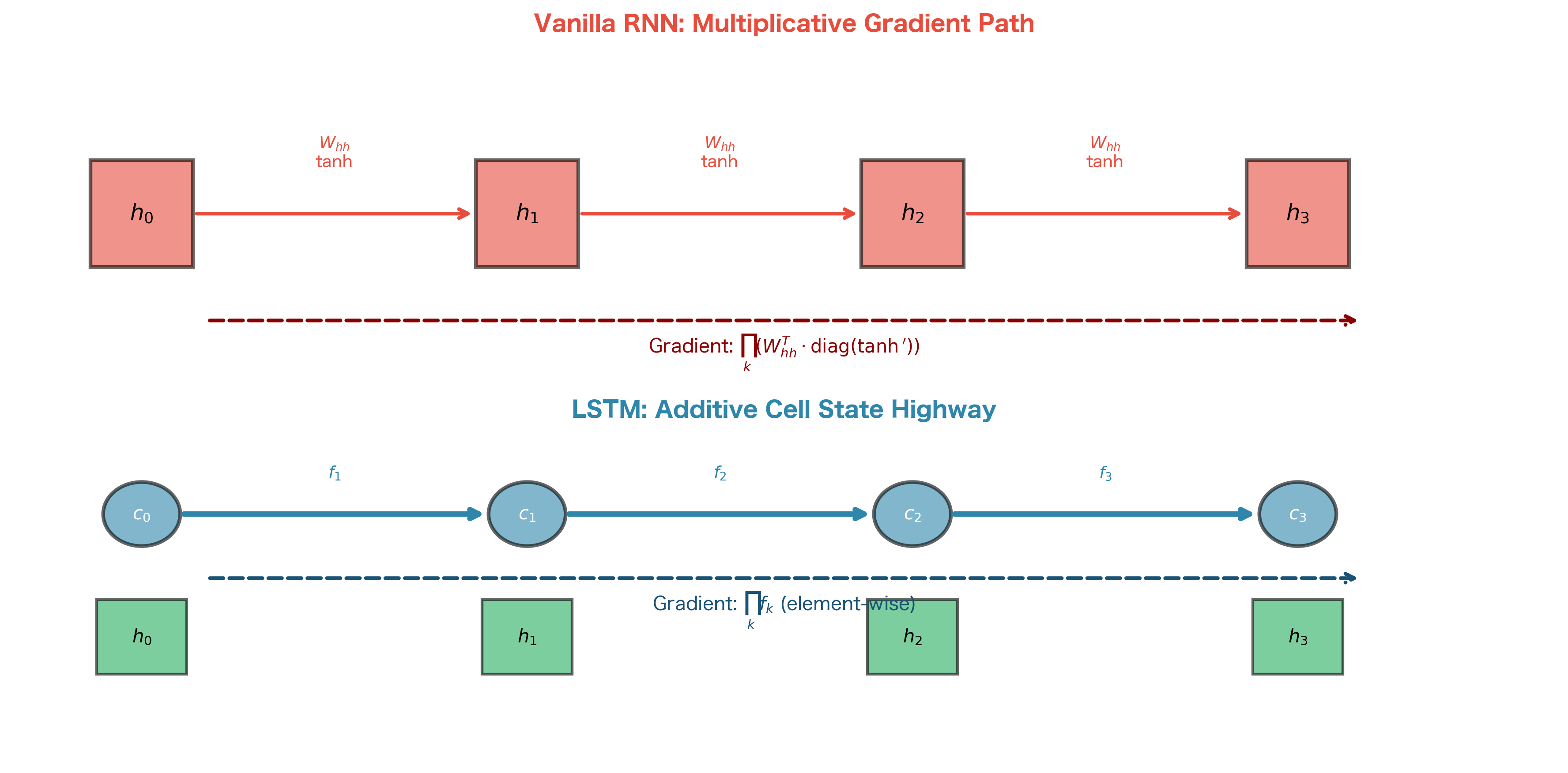
The crucial observation is that this update is additive with respect to the previous cell state. The previous cell state is scaled by the forget gate and then added to new information. Compare this to the vanilla RNN update:
where:
- : the hidden state at timestep
- : the recurrent weight matrix that transforms the previous hidden state
- : the hidden state from the previous timestep
- : the input weight matrix that transforms the current input
- : the input at timestep
- : the bias vector
- : the hyperbolic tangent activation function
In the vanilla RNN, the previous hidden state passes through a matrix multiplication and a nonlinearity at every timestep. In the LSTM, the cell state can flow through with only element-wise scaling by the forget gate.
Why Additive Updates Matter
The difference between multiplicative and additive updates might seem subtle, but it has profound implications for gradient flow. To understand why, we need to look at what happens during backpropagation.
During the backward pass, we compute how the loss changes with respect to earlier states. This requires the Jacobian , a matrix that tells us how each component of depends on each component of .
Starting from the cell state equation , we apply the chain rule:
This equation reveals something remarkable. The first term, , is a diagonal matrix with the forget gate values on its diagonal. This term comes directly from differentiating , the additive contribution of the previous cell state.
The second term captures how the new information () depends on . This dependency is indirect: affects , which affects the gates, which affect the update. We'll analyze this indirect path later.
The critical insight is that the first term provides a direct gradient path with three special properties:
- No weight matrices: Unlike vanilla RNNs, gradients don't pass through learned weight matrices on this path.
- No activation saturation: The path doesn't involve tanh or sigmoid derivatives that could shrink gradients.
- Learnable scaling: The forget gate values are learned, so the network can control gradient flow.
When the forget gate is close to 1, this term is approximately the identity matrix . In that case, gradients flow backward with minimal decay: the "constant error carousel" in action.
The constant error carousel refers to the LSTM's ability to maintain constant gradient flow through the cell state when the forget gate equals 1. In this limiting case, , and gradients propagate backward indefinitely without decay. The "carousel" metaphor evokes information cycling through time without degradation, like a carousel that keeps spinning without friction.
The Forget Gate as a Gradient Highway
The forget gate serves a dual purpose in LSTMs. In the forward pass, it controls how much of the previous cell state to retain. In the backward pass, it controls how much gradient flows to earlier timesteps. This duality is not coincidental: it's a fundamental property of how gradients work.
Deriving the Gradient
Let's make the gradient highway concrete with a formal derivation. Suppose we have a loss computed at the final timestep . We want to understand how gradients propagate backward, specifically how relates to .
Starting from the cell state update equation:
By the chain rule, the gradient with respect to has two components:
- Direct path: Gradients flow directly through the term
- Indirect paths: Gradients flow through , , and , all of which depend on , which in turn depends on
For now, let's focus on the direct path, which is the star of the show. The derivative of with respect to is simply (element-wise). So the direct path contribution is:
This equation is the heart of the LSTM's gradient flow. It says: the gradient at timestep equals the gradient at timestep , scaled element-wise by the forget gate. No weight matrices. No activation derivatives. Just a simple scaling.
Now consider what happens over multiple timesteps. If we trace the direct path from timestep back to timestep , the gradient accumulates as:
The product is computed element-wise, meaning each dimension of the cell state has its own chain of forget gates. This product determines how much gradient survives the journey backward through timesteps.
Here's the key insight: if all forget gates equal 1, the product equals 1, and gradients flow perfectly. If forget gates average 0.9, the product after 10 timesteps is , still substantial. Compare this to a vanilla RNN, where the equivalent factor involves weight matrix eigenvalues and tanh derivatives, typically yielding after 10 timesteps.
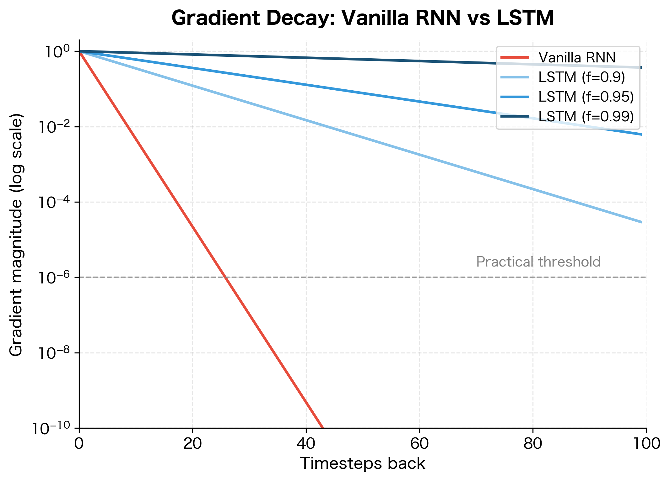
The visualization reveals a striking difference. The vanilla RNN's gradient decays below the practical threshold (where gradients become too small to provide useful learning signal) within about 15-20 timesteps. LSTMs with forget gates averaging 0.9 extend this to about 50 timesteps, while forget gates averaging 0.99 maintain useful gradients for over 100 timesteps.
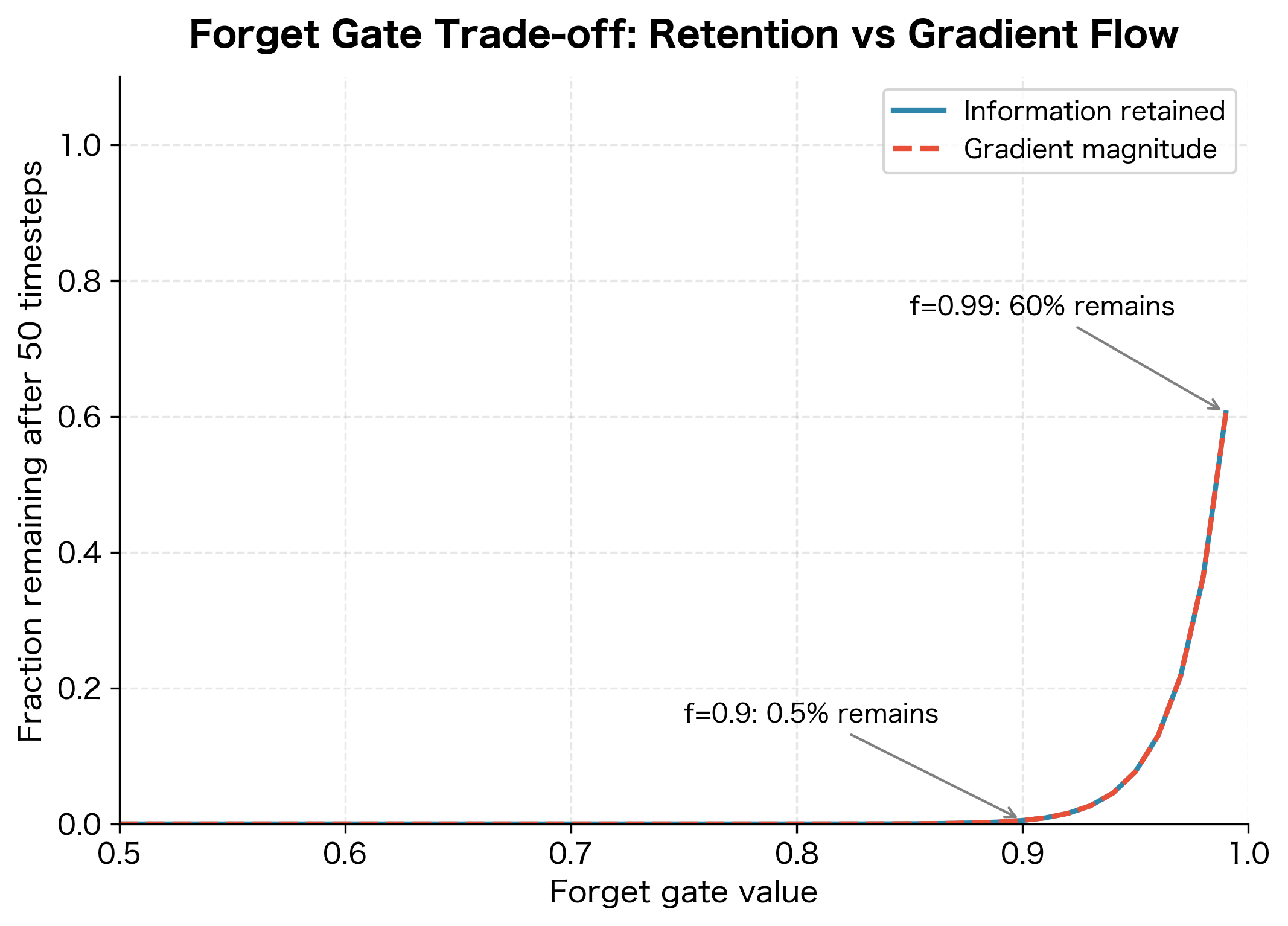
The Forget Gate Gradient Trade-off
There's an important trade-off in the forget gate's behavior. A forget gate close to 1 provides excellent gradient flow but prevents the network from forgetting old information. A forget gate close to 0 allows aggressive forgetting but blocks gradient flow.
In practice, well-trained LSTMs learn to balance this trade-off. The forget gate stays relatively high (preserving gradients) for information that needs to persist, and drops lower when the network needs to clear old state. This adaptive behavior emerges from training: the network learns forget gate patterns that both maintain useful information and enable learning.
Complete Gradient Flow Analysis
So far, we've focused on the direct gradient path through the forget gate, the "gradient highway" that makes LSTMs so effective. But this is only part of the story. To fully understand LSTM gradient flow, we need to trace all the paths gradients can take as they propagate backward through time.
Think of it this way: when we compute , we're asking "how does a small change in the previous cell state affect the loss?" The answer involves multiple routes:
- The direct route: The previous cell state directly contributes to the current cell state through the forget gate multiplication.
- The indirect routes: The previous cell state also affects the hidden state , which in turn influences all the gates at timestep , which then affect the cell state update.
Let's derive the complete picture.
The Full Jacobian
To capture all gradient paths, we need the complete Jacobian . Using the chain rule, this decomposes into:
The first term, , is a diagonal matrix with the forget gate values on its diagonal. This is the direct path we analyzed earlier: simple, stable, and controlled entirely by the forget gate.
The second term represents the indirect paths. It's a product of two Jacobians:
- : How does the current cell state depend on the previous hidden state? This captures the influence through all three gates.
- : How does the previous hidden state depend on the previous cell state? This is the output gate and tanh connection.
Expanding the Indirect Paths
Let's work through each piece. The cell state update is:
The previous hidden state affects this update through three channels: it influences , , and . Taking the derivative with respect to :
Each term corresponds to one gate's contribution:
| Term | Gate | Meaning |
|---|---|---|
| Forget | How changes in affect what we keep from the past | |
| Input | How changes in affect how much new information we add | |
| Candidate | How changes in affect what new information we propose |
The second piece connects the hidden state to the cell state. Recall that . Taking the derivative:
This is a product of two diagonal matrices:
- : The output gate values, all between 0 and 1
- : The tanh derivative, also between 0 and 1
Notice that both factors are bounded between 0 and 1, so this product tends to shrink gradients. This is a key observation we'll return to.
Why the Direct Path Dominates
Now we can see why the LSTM's gradient flow is so much better than a vanilla RNN's. Compare the two gradient paths:
Direct path ():
- Involves only element-wise scaling by the forget gate
- No weight matrices
- No activation function derivatives (other than the forget gate's sigmoid, which is already folded into )
- Controlled entirely by the learned forget gate values
Indirect paths ():
- Involve products of weight matrices (through , etc.)
- Multiplied by the tanh derivative, which is at most 1 and often much smaller
- Multiplied by the output gate, which is at most 1
- Subject to the same vanishing/exploding gradient problems as vanilla RNNs
This leads to two crucial insights:
-
Magnitude: The direct path gradient is simply , which the network learns to keep near 1 for important information. The indirect paths involve products of many terms, each bounded by 1, so they tend to be much smaller.
-
Stability: The direct path doesn't involve any learned weight matrices; it's purely controlled by the forget gate. The indirect paths pass through weight matrices that can have problematic eigenvalues, but because they're multiplied by small factors (tanh derivatives, output gates), their contribution is usually dominated by the stable direct path.
Let's verify this empirically. First, we can measure the actual forget gate values in a trained LSTM and visualize them as a heatmap:
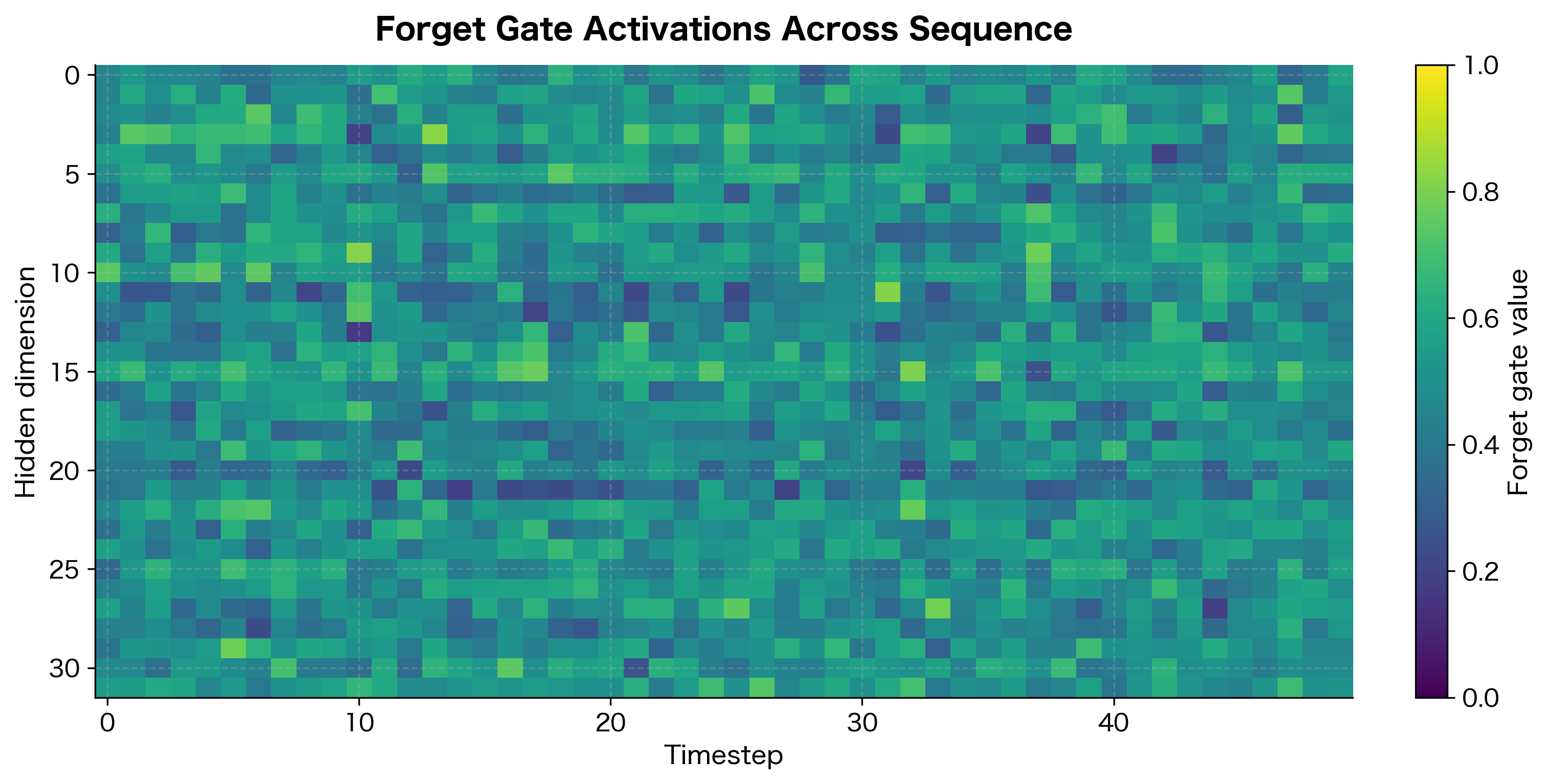
The heatmap reveals the forget gate landscape. With default initialization, values cluster around 0.5, but trained LSTMs learn to push these higher for dimensions storing important long-term information. The variation across hidden dimensions shows how different "memory slots" can have different retention characteristics.
Now let's measure actual gradient magnitudes in a trained LSTM:
LSTM vs Vanilla RNN: A Direct Comparison
Let's directly compare gradient flow in vanilla RNNs and LSTMs on the same task. We'll use a simple memory task where the network must remember information from early in the sequence.
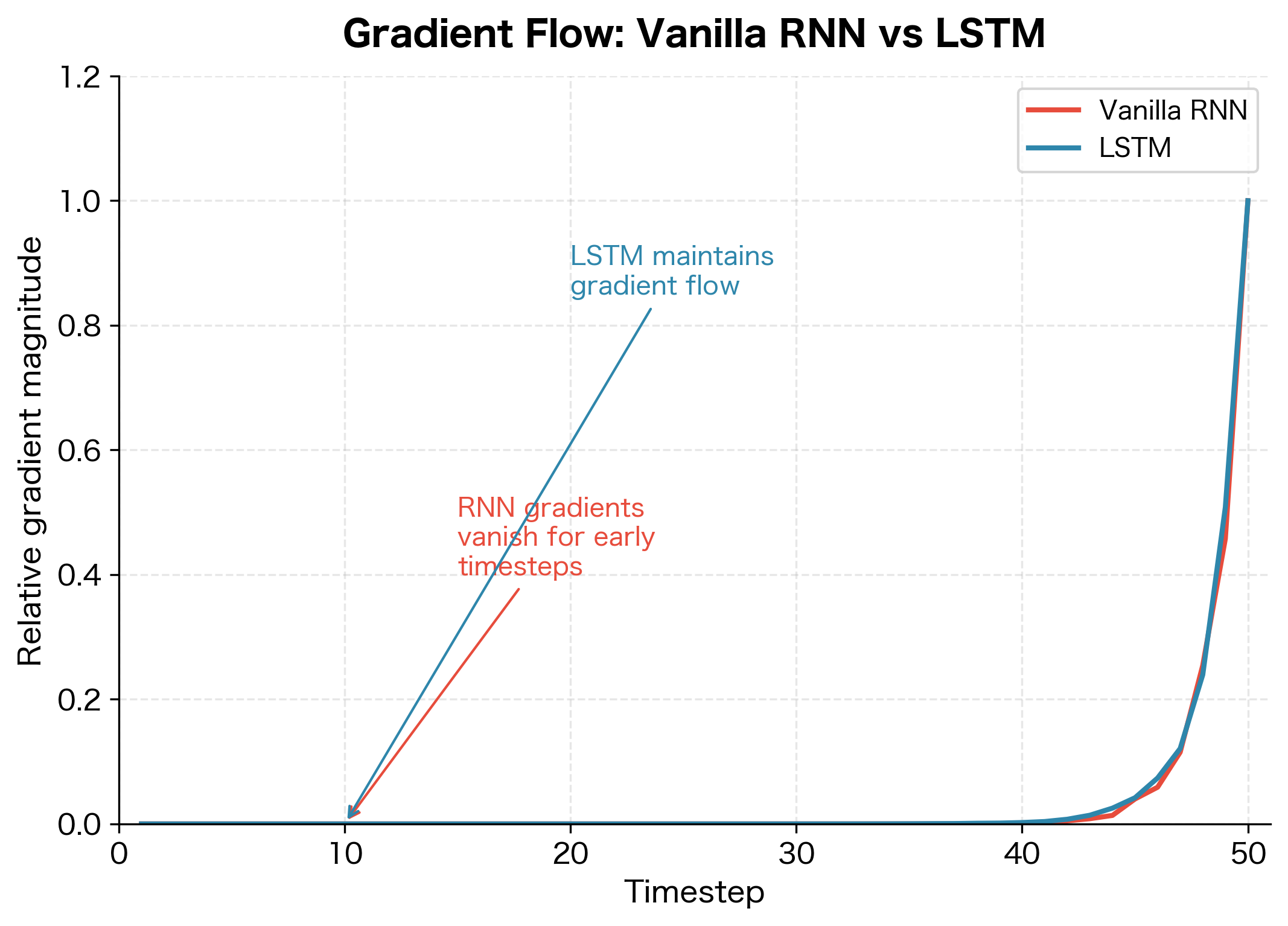
The comparison reveals the LSTM's advantage clearly. While the vanilla RNN's gradients decay rapidly as we move earlier in the sequence, the LSTM maintains relatively stable gradient flow throughout. This is why LSTMs can learn dependencies spanning 50, 100, or even more timesteps, while vanilla RNNs struggle beyond 10-20 timesteps.
Visualizing the Gradient Distribution
Another way to see the difference is to look at the distribution of gradient magnitudes across all timesteps. For a vanilla RNN, we expect a heavily skewed distribution with most gradients near zero. For an LSTM, we expect a more uniform distribution:
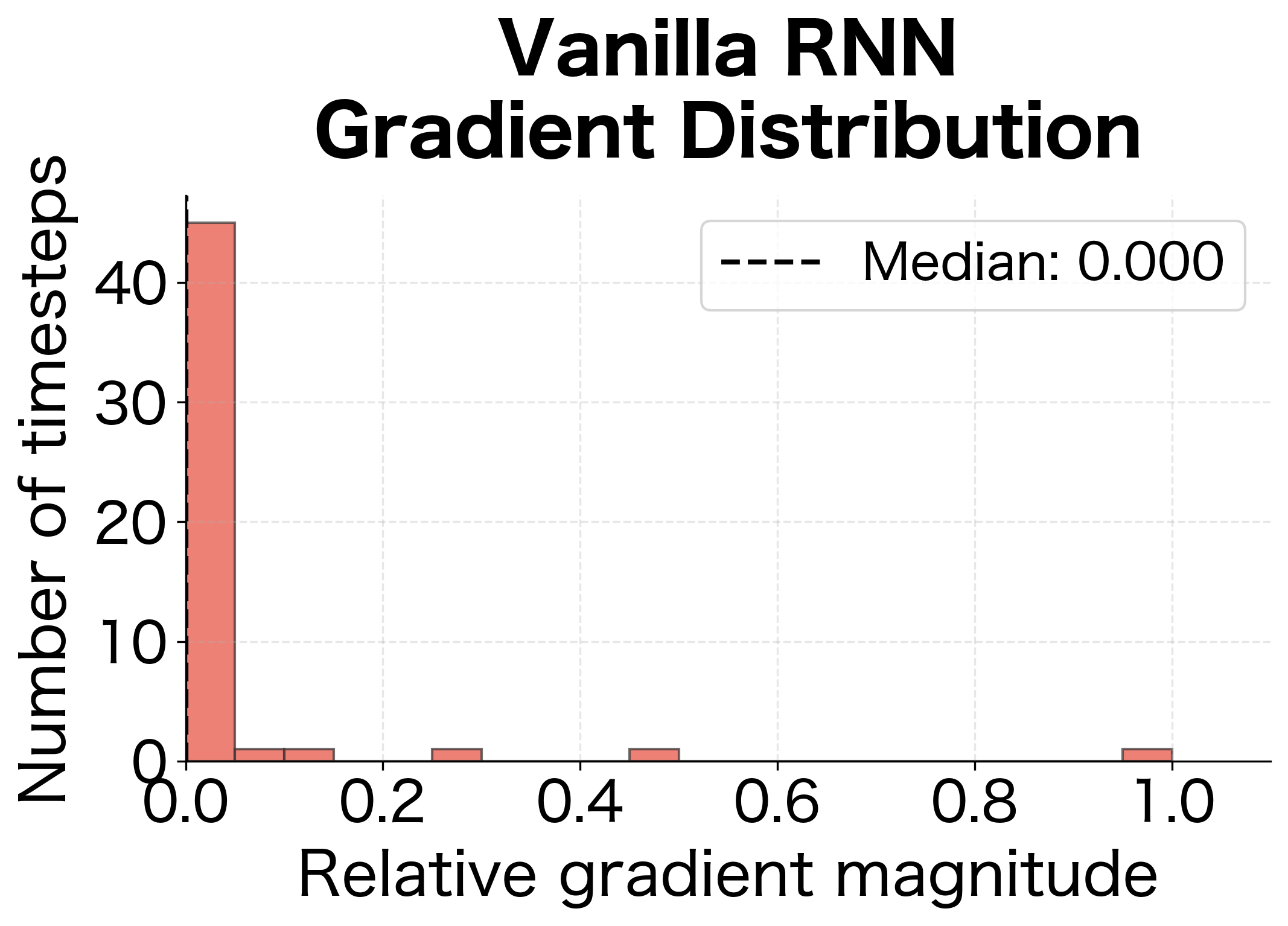
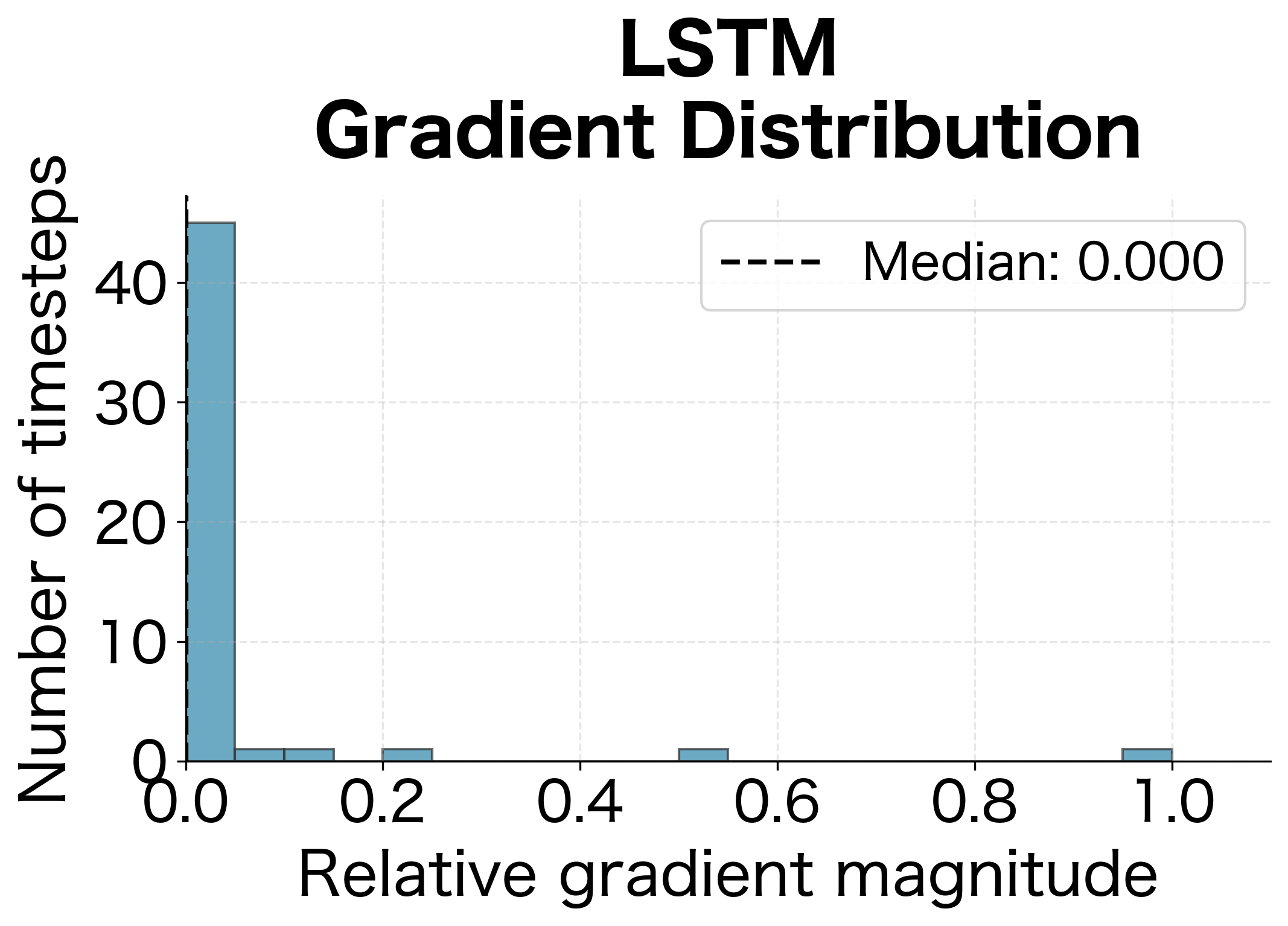
The distributions tell a clear story. The vanilla RNN's gradient distribution is heavily skewed toward zero, meaning most timesteps receive negligible gradient signal. The LSTM's distribution is much more uniform, with the median gradient magnitude significantly higher. This uniformity is what enables LSTMs to learn from early parts of the sequence.
Quantifying the Difference
Let's quantify exactly how much better LSTMs are at preserving gradients:
The metrics confirm what we see visually. The first/last gradient ratio measures how much gradient reaches the earliest timestep compared to the final timestep, where higher values indicate better gradient flow to early timesteps. The coefficient of variation captures how uniformly gradients are distributed across timesteps, where lower values mean more uniform distribution, which is desirable for learning long-range dependencies. The effective range counts how many timesteps receive at least 10% of the maximum gradient, where more timesteps means gradients remain useful across a larger portion of the sequence. The LSTM's first-to-last gradient ratio is much higher, meaning gradients reach early timesteps more effectively. The coefficient of variation is lower, indicating more uniform gradient distribution. And the effective range shows that LSTM gradients remain useful across nearly all timesteps, while RNN gradients are only useful for a fraction of the sequence.
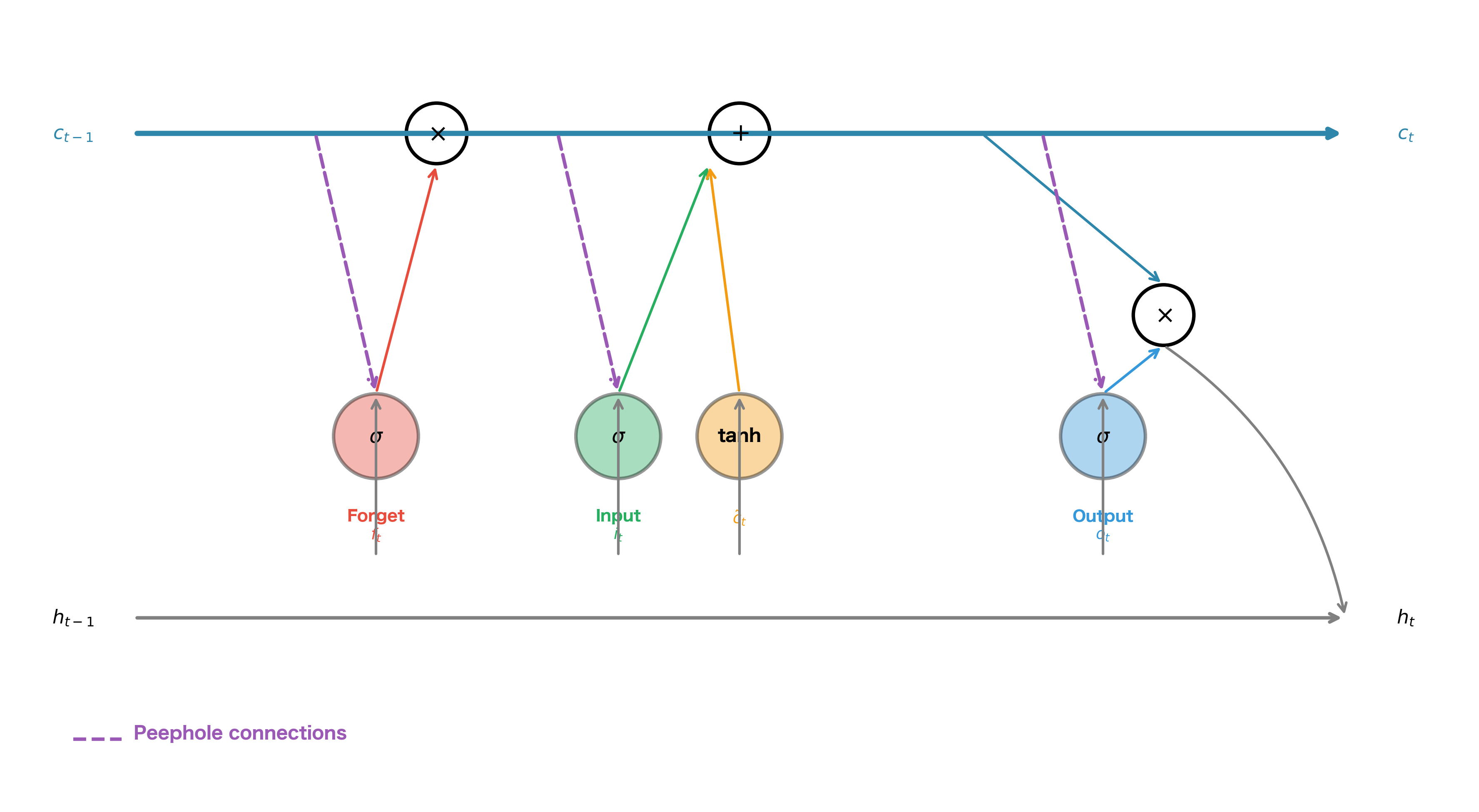
Peephole Connections
Standard LSTMs compute gate activations based on the current input and previous hidden state . Peephole connections, introduced by Gers and Schmidhuber in 2000, allow gates to also directly observe the cell state. This can improve the network's ability to learn precise timing.
The Peephole Equations
With peephole connections, each gate receives an additional input: a direct view of the cell state. The standard gate computation is augmented with a term , where is a learnable weight vector and is the cell state. The modified gate equations become:
where:
- : input weight matrices (same as standard LSTM)
- : recurrent weight matrices (same as standard LSTM)
- : peephole weight vectors for forget, input, and output gates
- : the previous cell state (used by forget and input gates)
- : the current cell state (used by output gate)
- : bias vectors
- : the sigmoid activation function
- : element-wise multiplication (the peephole weights are vectors, not matrices)
Notice that the forget and input gates use the previous cell state , while the output gate uses the current cell state . This is because the output gate needs to see the updated cell state to decide what to output. The peephole weights are vectors rather than matrices, meaning each gate dimension only sees the corresponding cell state dimension . This keeps the parameter count low: peepholes add only parameters (one vector per gate) rather than parameters that matrices would require.
Peephole connections add direct connections from the cell state to the gates, allowing gates to make decisions based on the actual memory content rather than just the filtered hidden state. The peephole weights are vectors (not matrices), so they add only parameters to the model.
Gradient Flow with Peepholes
Peephole connections create additional gradient paths. The gradient now flows not only through the forget gate scaling but also through the peephole connections themselves. This can provide additional gradient highways, potentially improving gradient flow for certain tasks.
However, peephole connections also make the gradient flow more complex. The cell state now directly influences the gates, which influence the cell state update, creating a more intricate dependency structure.
When to Use Peepholes
Peephole connections are most useful when:
- Precise timing matters: Tasks like rhythm detection or time series prediction with specific periodicities benefit from gates being able to see the exact cell state values.
- Cell state magnitude is informative: When the absolute value of stored information matters, not just its presence or absence.
- Standard LSTM underperforms: If a standard LSTM struggles with a task despite adequate capacity, peepholes might help.
However, peepholes add complexity and computation. In practice, many successful applications use standard LSTMs without peepholes. The GRU architecture, which we'll cover in a later chapter, takes a different approach by simplifying the gating mechanism rather than adding peepholes.
Gradient Clipping in LSTMs
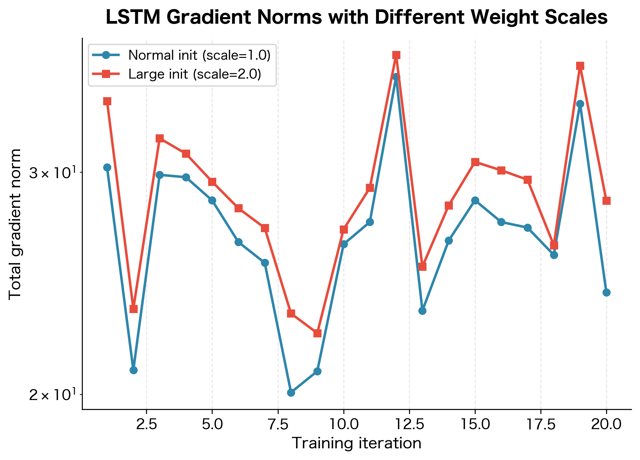
Despite the cell state gradient highway, LSTMs can still experience exploding gradients. This happens primarily through the indirect gradient paths: the gates depend on weight matrices, and if these weights have large eigenvalues, gradients can explode.
When Gradients Explode in LSTMs
Exploding gradients in LSTMs typically occur when:
-
Weight matrices have large spectral radius: The gate weight matrices , , , transform the hidden state. If their eigenvalues exceed 1, gradients through the indirect paths can explode.
-
Long sequences with active gates: When the input and forget gates are both active (not saturated near 0 or 1), gradients flow through multiple paths and can accumulate.
-
Poor initialization: Random initialization can create weight matrices with problematic eigenvalue distributions.
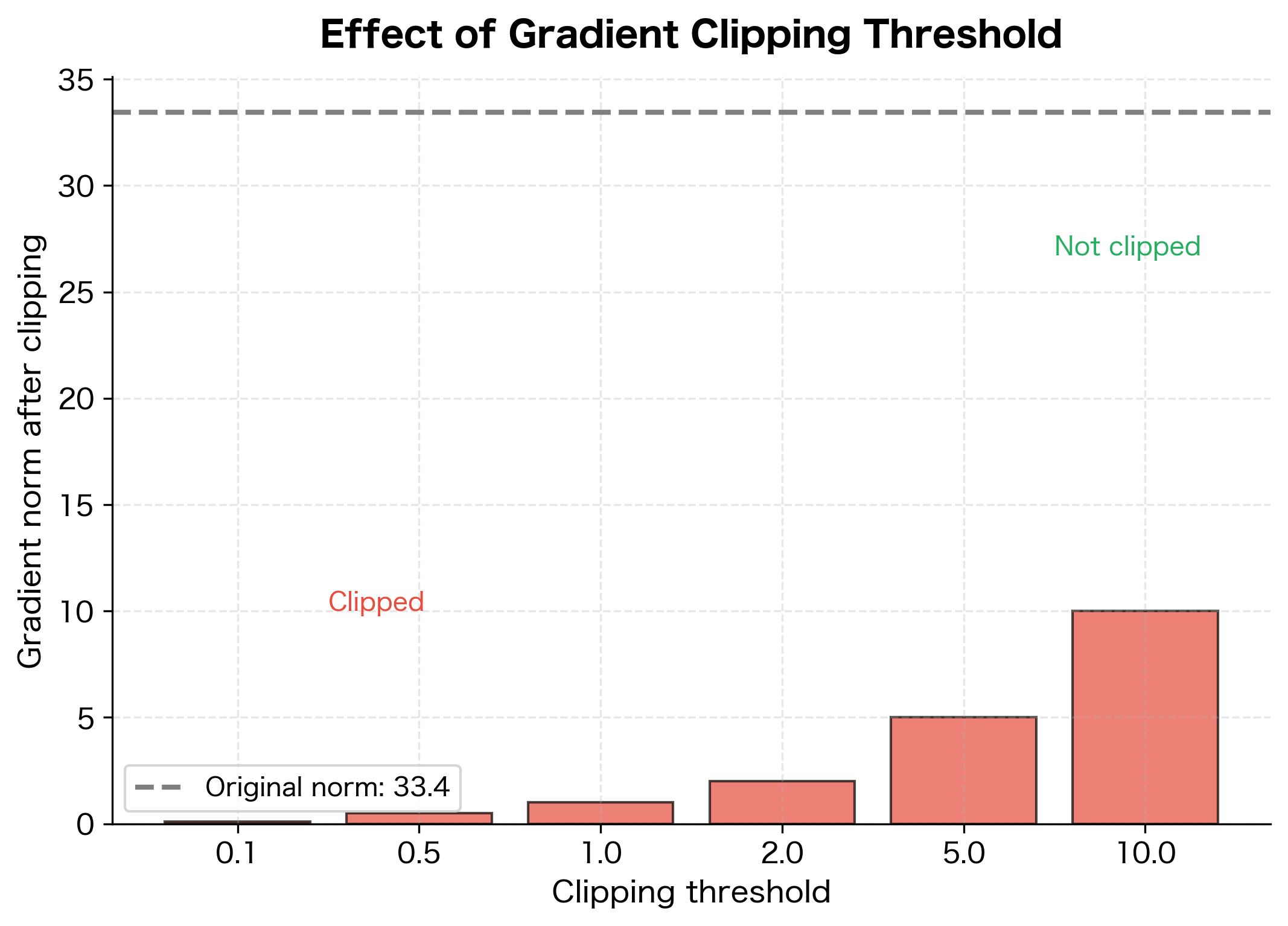
Implementing Gradient Clipping
Gradient clipping is a standard technique that rescales gradients when their norm exceeds a threshold. For LSTMs, this is typically applied to all parameters together:
The gradient norm before clipping indicates how large the gradients grew during this backward pass. When this exceeds the threshold (1.0 in this case), the gradients are scaled down proportionally so their norm equals exactly the threshold. The clipping ratio shows what fraction of the original gradient magnitude is retained. A ratio of 1.0 means no clipping occurred, while smaller values indicate more aggressive scaling. This prevents any single update from being too large, which could destabilize training.
Choosing the Clipping Threshold
The gradient clipping threshold is a hyperparameter that requires tuning. Common practices include:
- Start with 1.0 or 5.0: These are reasonable defaults for most tasks.
- Monitor gradient norms: Log gradient norms during training to understand the typical range.
- Adjust based on stability: If training is unstable (loss spikes), reduce the threshold. If training is too slow, try increasing it.
Worked Example: Tracing Gradients Through an LSTM
The mathematical analysis above tells us why LSTM gradients flow better, but there's no substitute for working through a concrete example. Let's trace gradient flow step by step through a small LSTM, computing every number explicitly so we can see the gradient highway in action.
Setting Up the Problem
We'll use deliberately small dimensions so every value is visible:
- Hidden dimension: (just two neurons)
- Sequence length: (three timesteps)
- Goal: Compute , which tells us how the initial cell state affects the final loss
This setup lets us trace the gradient as it flows backward through time: from to to to . At each step, we'll see the forget gate scaling the gradient, creating the "highway" effect.
To keep the example tractable, we'll use fixed gate values rather than computing them from weights. In a real LSTM, these would be learned, but the gradient flow mechanics are identical.
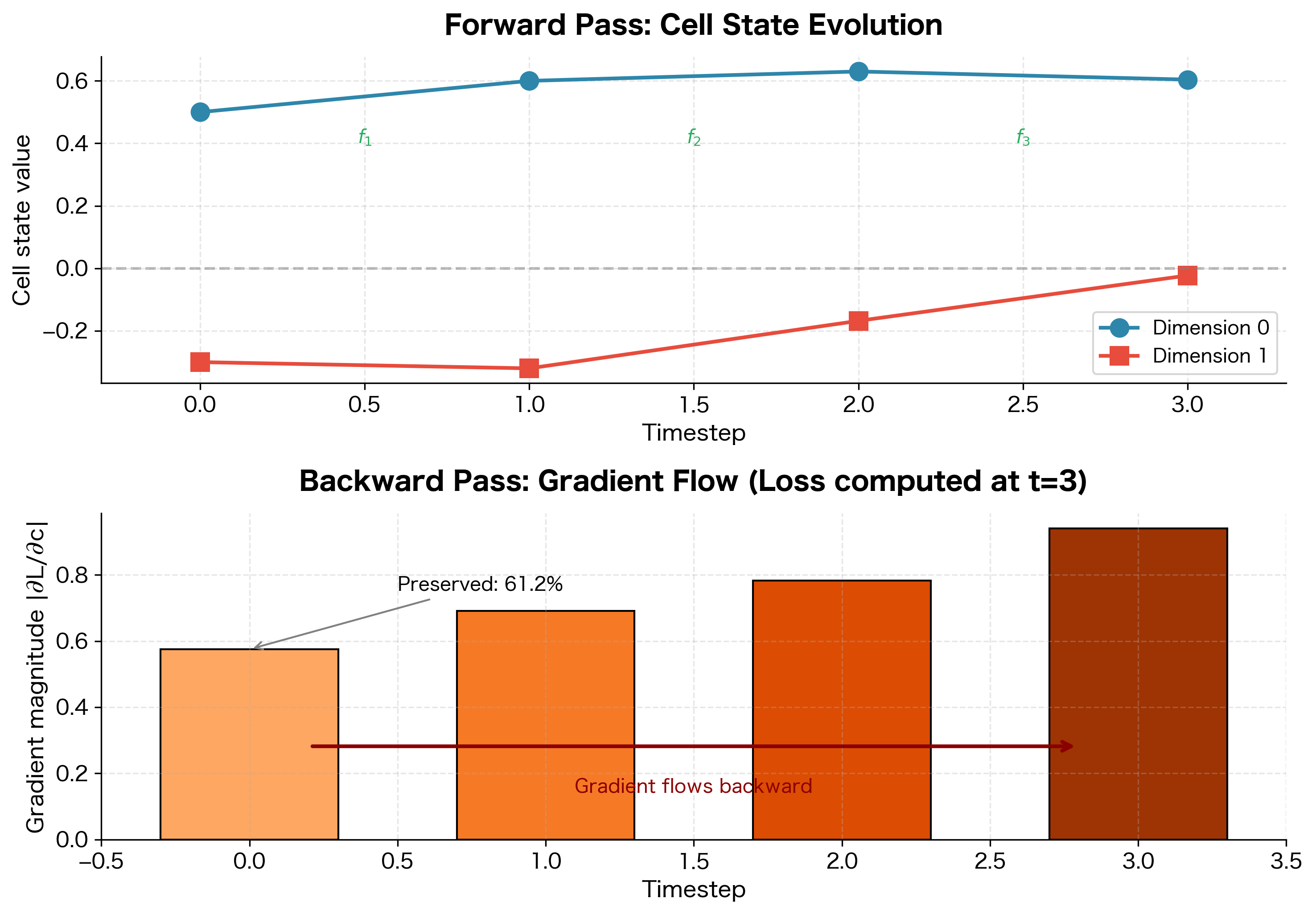
Interpreting the Results
The output reveals the gradient highway in action. Let's trace through what happened:
Forward pass: Starting from , the cell state evolved through three timesteps. At each step, the forget gate scaled the previous state and the input gate added new information. The final cell state fed into the output gate to produce , which determined the loss.
Backward pass: The gradient started at (since our loss was the sum of ). It then flowed backward through:
- The output gate and tanh, giving
- The forget gate , giving
- The forget gate , giving
- The forget gate , giving
The key insight: The cumulative forget gate product tells us what fraction of the gradient survives the journey. With forget gates averaging around 0.85, we preserve about 61% of the gradient magnitude over just 3 timesteps.
Compare this to a vanilla RNN, where the equivalent factor would be approximately , only 20% preserved. Over longer sequences, this difference becomes dramatic: after 10 timesteps, the LSTM preserves roughly 20% () while the vanilla RNN preserves less than 0.5% ().
Limitations and Impact
Understanding gradient flow in LSTMs reveals both their strengths and remaining limitations.
What LSTMs Achieve
The constant error carousel and forget gate gradient highway enable LSTMs to learn dependencies spanning hundreds of timesteps. This was revolutionary when introduced in 1997 and enabled breakthroughs in speech recognition, machine translation, and language modeling throughout the 2000s and 2010s. The key insight that additive updates preserve gradients better than multiplicative updates has influenced subsequent architectures, including residual networks and transformers.
Remaining Limitations
Despite improved gradient flow, LSTMs face several challenges:
Gradient decay still occurs: Even with forget gates near 1, gradients decay as over timesteps, where is the average forget gate value and is the sequence length. For very long sequences (thousands of tokens), this decay becomes significant. The forget gate cannot be exactly 1 everywhere, or the network would never forget anything.
Sequential computation bottleneck: LSTMs must process sequences one timestep at a time because each hidden state depends on the previous one. This prevents parallelization across time, making LSTMs slow on modern GPUs optimized for parallel computation. Transformers address this by processing all positions in parallel.
Limited context window in practice: While theoretically capable of infinite context, practical LSTMs struggle with dependencies beyond a few hundred timesteps. The attention mechanism in transformers provides a more direct way to connect distant positions.
Complexity of gradient paths: The full gradient flow involves not just the direct path through the forget gate but also indirect paths through all the gates. These indirect paths can still experience vanishing or exploding gradients, requiring careful initialization and gradient clipping.
Summary
This chapter analyzed gradient flow in LSTMs, revealing why they succeed where vanilla RNNs fail.
The Constant Error Carousel:
The cell state update is additive with respect to the previous cell state. This creates a direct gradient path where the Jacobian of the cell state with respect to the previous cell state is:
where is a diagonal matrix with forget gate values on the diagonal, and the indirect paths represent gradient flow through the gates (which depend on the previous hidden state). When the forget gate is close to 1, the diagonal matrix approaches the identity matrix, allowing gradients to flow backward with minimal decay.
The Forget Gate Gradient Highway:
Over timesteps, the direct path gradient scales as , where the product is taken element-wise over all forget gate vectors from timestep 1 to . With forget gates averaging 0.9, gradients retain about 35% of their magnitude over 10 timesteps (since ), compared to less than 1% for vanilla RNNs.
Key Insights:
- The same mechanism that preserves information (high forget gate) also preserves gradients
- Peephole connections add direct cell state observation to gates, creating additional gradient paths
- LSTMs still need gradient clipping because indirect paths through weight matrices can explode
- The gradient highway enables learning dependencies spanning hundreds of timesteps, but very long sequences still pose challenges
Practical Implications:
- Initialize forget gate bias to 1 or higher to start with good gradient flow
- Use gradient clipping (typically max norm 1.0-5.0) to handle exploding gradients through indirect paths
- For very long sequences (1000+ tokens), consider attention mechanisms or hierarchical approaches
The next chapter explores the GRU architecture, which simplifies the LSTM's gating mechanism while maintaining effective gradient flow.
Key Parameters
When working with LSTMs and considering gradient flow, several parameters significantly impact training stability:
-
forget_bias (initialization): The initial value for the forget gate bias. Setting this to 1.0 or higher ensures the network starts with good gradient flow by keeping forget gates near 1. This is one of the most important initialization choices for LSTMs.
-
gradient_clip_norm (
max_normin PyTorch'sclip_grad_norm_): The maximum allowed gradient norm. Values of 1.0-5.0 are typical. Lower values provide more stability but may slow learning; higher values allow faster updates but risk instability. -
hidden_size: Larger hidden dimensions mean more gradient paths (both direct and indirect). While the direct path scales linearly, indirect paths involve larger weight matrices that may have more extreme eigenvalues.
-
num_layers: Stacked LSTMs have gradient flow challenges between layers as well as across time. Residual connections between layers can help preserve gradients in deep LSTMs.
-
weight_init_scale: The scale of weight initialization affects the spectral radius of recurrent weight matrices. Xavier or orthogonal initialization helps maintain stable gradient flow through indirect paths.
-
sequence_length: Longer sequences require gradients to flow through more timesteps. Even with the cell state highway, very long sequences (1000+ tokens) may experience significant gradient decay.
Quiz
Ready to test your understanding? Take this quick quiz to reinforce what you've learned about LSTM gradient flow and the constant error carousel.

Comments