

Learn how NTK-aware scaling extends transformer context windows by preserving high-frequency position information while scaling low frequencies for longer sequences.

This article is part of the free-to-read Language AI Handbook
Choose your expertise level to adjust how many terms are explained. Beginners see more tooltips, experts see fewer to maintain reading flow. Hover over underlined terms for instant definitions.
NTK-aware Scaling
Position Interpolation, as we saw in the previous chapter, extends context length by simply scaling down all rotation frequencies. While this works, it comes with a hidden cost: by compressing all frequencies equally, we lose the fine-grained positional distinctions that high-frequency components provide. Consider a model trained with 4,096 tokens. Position Interpolation at 8x scale compresses everything to fit 32,768 positions, but now adjacent tokens that were once easily distinguishable become nearly identical in their high-frequency dimensions.
NTK-aware scaling takes a more surgical approach. Instead of treating all frequencies equally, it recognizes that different frequency bands serve different purposes. High frequencies distinguish nearby tokens, while low frequencies capture long-range structure. By scaling frequencies non-uniformly, NTK-aware methods preserve local precision while still extending the effective context window.
This chapter develops the intuition behind NTK-aware scaling, derives the mathematical formula, and implements both static and dynamic variants. By the end, you'll understand why this approach often outperforms linear interpolation, especially for tasks requiring precise local attention.
The Problem with Uniform Scaling
To understand why uniform scaling falls short, we need to revisit how RoPE frequencies work. Recall that RoPE assigns each dimension pair a base frequency that determines how fast the rotation angle changes with position:
where:
- : the base rotation frequency (in radians per position) for dimension pair
- : the base constant, typically 10000, which controls the overall frequency range
- : the dimension pair index, ranging from 0 to
- : the total embedding dimension (must be even since we work in pairs)
- : the exponent that creates a geometric progression of frequencies across dimensions
The first dimension pair () has frequency , meaning it rotates by 1 radian per position and completes a full rotation every positions. The last pair () has a much smaller frequency, completing a rotation only after thousands of positions. This spread creates a multi-scale representation:
- High-frequency pairs ( near 0): Distinguish nearby tokens with precision. Tokens at positions 5 and 6 look very different.
- Low-frequency pairs ( near ): Capture coarse position information. Tokens far apart have noticeably different rotations.
Position Interpolation addresses context extension by scaling all frequencies uniformly:
where:
- : the scaled frequency for dimension pair after Position Interpolation
- : the original frequency for dimension pair
- : the context extension factor, computed as (target length divided by training length)
If we want to extend from 4,096 to 32,768 tokens, . Every frequency gets divided by 8. The high-frequency pair that previously rotated 1 radian per position now rotates only radians. Adjacent tokens, which were once clearly distinguishable, become nearly indistinguishable in these dimensions.
Let's visualize this problem:
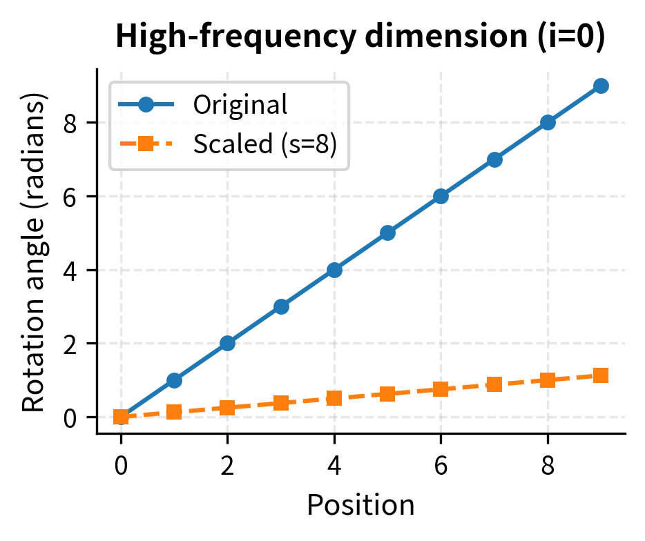
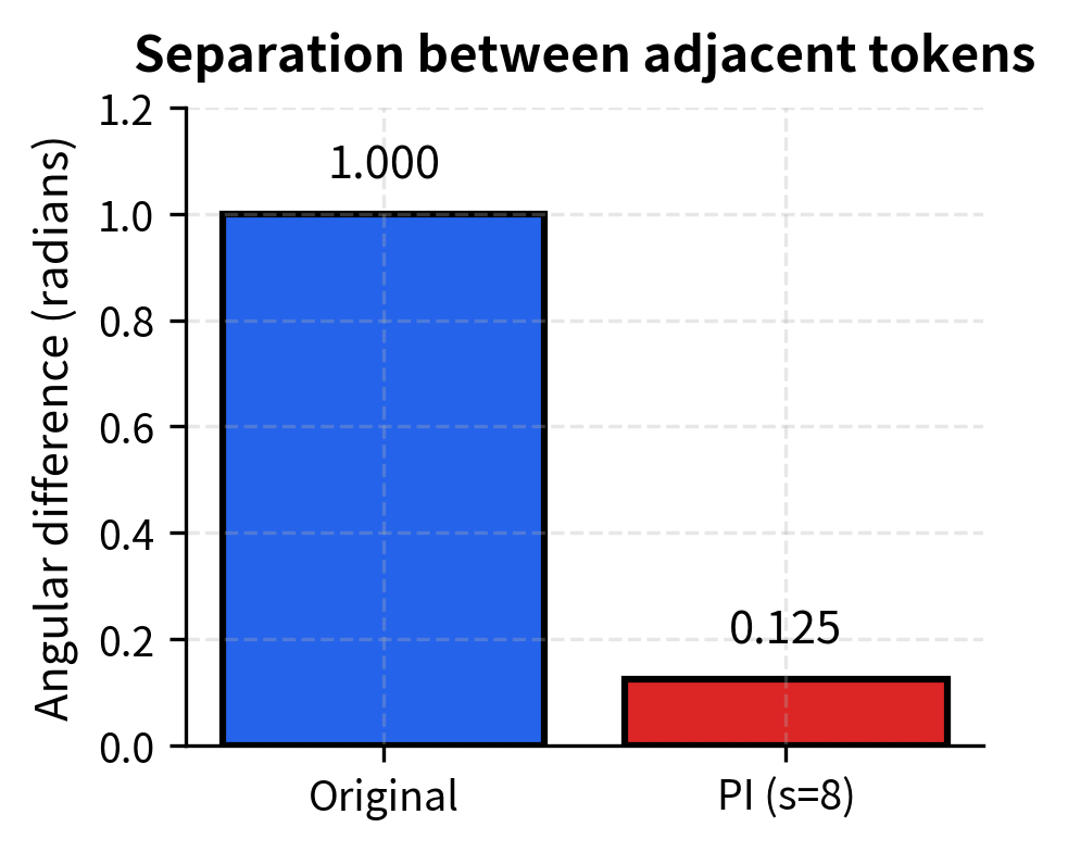
The compression is dramatic. With Position Interpolation at 8x scale, adjacent tokens are separated by only 0.125 radians in the highest-frequency dimension, compared to 1 radian originally. This means the model has far less "room" to distinguish nearby positions, potentially harming tasks that require precise local attention.
From Intuition to Formula: The NTK-aware Approach
Now that we've seen the problem with uniform scaling, let's develop a solution from first principles. The journey from intuition to a working formula requires answering three questions: What property do we want? How can we achieve it mathematically? And does the result match our expectations?
The Neural Tangent Kernel describes how neural networks behave during training in the infinite-width limit. In this context, "NTK-aware" refers to preserving the high-frequency components that the network needs to learn fine-grained distinctions between nearby positions.
The Core Insight: Frequency Bands Serve Different Purposes
The key realization is that not all frequencies are equal in importance. Think of RoPE's multi-frequency design like a ruler with both centimeter and millimeter markings. The millimeter marks (high frequencies) give you precision for small measurements, while the centimeter marks (low frequencies) help you measure longer distances quickly. Position Interpolation is like shrinking the entire ruler by 8x, making even the millimeter marks too small to read. What we really want is to keep the millimeter precision while adjusting the centimeter scale.
Translating this intuition into concrete requirements:
-
Preserve high frequencies: The fastest-rotating dimension pairs (small ) should remain unchanged. These are our "millimeter marks" for local position distinctions.
-
Scale low frequencies: The slowest-rotating dimension pairs (large ) can be compressed by the full factor . These are our "centimeter marks" that need adjustment for longer contexts.
-
Smooth transition: Intermediate dimensions should scale gradually between these extremes, not abruptly jump.
Designing the Solution: Modify the Base
How can we achieve dimension-dependent scaling? The original RoPE frequency formula is . Position Interpolation modifies the output by dividing: . This gives uniform scaling because every frequency is divided by the same constant.
Instead, we'll modify the input: the base . If we replace with a larger base , all frequencies decrease (slower rotation). The key insight is that the exponent causes this decrease to affect different dimensions differently:
- When : . No matter what is, the highest frequency remains 1.
- When is large: shrinks more because the exponent is larger.
This is exactly the property we want! By choosing the right , we can leave high frequencies untouched while scaling low frequencies by whatever factor we need.
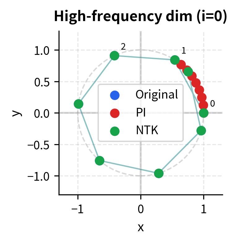
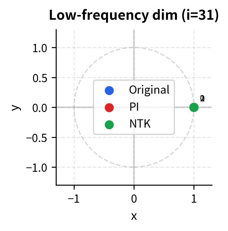
This geometric view makes the difference concrete. In the high-frequency dimension (left), original RoPE spreads positions around the circle, allowing the model to distinguish them easily. Position Interpolation bunches them together near the starting point, reducing distinguishability. NTK-aware scaling preserves the original spread. In the low-frequency dimension (right), all methods behave similarly since both Position Interpolation and NTK-aware apply full compression to these slow-rotating dimensions.
Deriving the Formula
Let's work backward from our requirements to find the exact formula for . We want a scaling function where:
- (no scaling at highest frequency)
- (full scaling at lowest frequency)
Let for some multiplier we need to determine. Substituting into the frequency formula:
Using the exponent rule , we can separate this:
The effective scaling factor for dimension becomes:
Now we apply our constraints. At , we need :
This is automatically satisfied for any , since any number raised to zero equals one. Our first requirement is met regardless of what we choose.
At (the last dimension pair), we need :
Simplifying the exponent step by step:
To solve for , we raise both sides to the power :
This gives us the complete NTK-aware formula:
where:
- : the modified base for NTK-aware scaling
- : the original base (typically 10000)
- : the context extension factor (e.g., to extend from 4k to 32k tokens)
- : the embedding dimension
- : an exponent slightly greater than 1 (for , this equals )
Understanding the Resulting Frequencies
Substituting the new base into the frequency formula reveals how each dimension is affected:
The effective scaling factor for each dimension is:
Let's verify this matches our design goals:
- When (highest frequency): . The highest frequencies are not scaled at all. ✓
- When (lowest frequency): . The lowest frequencies are scaled by the full factor. ✓
- Intermediate dimensions: Scaling increases smoothly from 1 to as increases. ✓
This is precisely what we wanted: high frequencies preserved, low frequencies scaled, smooth transition between.
A Worked Example
Let's make this concrete with typical values: dimensions, extension factor (4k to 32k tokens).
First, compute the NTK exponent:
The modified base becomes:
Now we can compute scaling factors for specific dimensions:
| Dimension | Exponent | Interpretation | |
|---|---|---|---|
| 0 | 0 | 1.00 | No scaling (preserved) |
| 8 | 0.258 | 1.72 | Slight scaling |
| 16 | 0.516 | 2.95 | Moderate scaling |
| 24 | 0.774 | 5.06 | Significant scaling |
| 31 | 1.00 | 8.00 | Full scaling |
The gradient is smooth and continuous. High-frequency pairs (small ) stay close to their original values, while low-frequency pairs (large ) are compressed to fit the extended context.
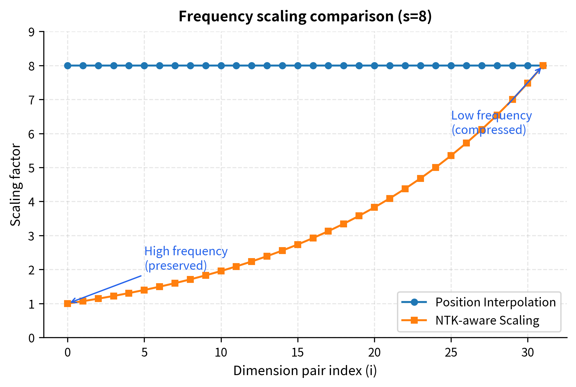
The visualization confirms our mathematical analysis. The NTK-aware curve (squares) starts at 1 for the highest-frequency pairs and smoothly increases to the full scale factor of 8 for the lowest-frequency pairs. Meanwhile, Position Interpolation (circles) maintains a flat line at 8, treating all dimensions identically.
Implementation
With the formula derived and verified, let's translate it into code. We'll build the implementation in layers, starting with the core frequency computation and progressively adding the full RoPE transformation.
Computing Frequencies
The foundation is a function that computes RoPE frequencies for any base value. This same function serves both the original frequencies and NTK-aware frequencies, since the only difference is the base we pass in:
Position Interpolation simply divides all frequencies by the scale factor:
NTK-aware scaling modifies the base according to our derived formula, then computes frequencies using the modified base:
Comparing the Approaches
Let's compute frequencies for all three methods and compare them side by side:
The numbers confirm what we derived mathematically. Look at the "PI ratio" column: it's a constant 8.00 across all dimensions, reflecting Position Interpolation's uniform scaling. Now look at "NTK ratio": it starts near 1.00 for dimension 0 and gradually increases toward 8.00 for the highest dimensions. This is the dimension-dependent scaling in action.
Visualizing the Frequency Spectrum
A log-scale plot reveals the full picture across all 32 dimension pairs:
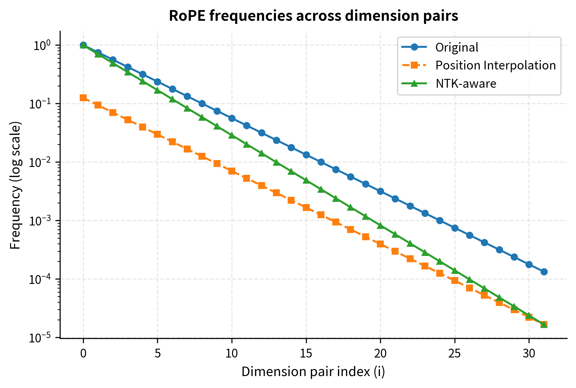
On the log scale, observe how NTK-aware frequencies (triangles) track the original (circles) closely for low dimension indices, where high frequencies live. As we move right toward higher dimension indices (lower frequencies), the NTK curve gradually diverges to match Position Interpolation (squares). This is exactly the "preserve high frequencies, scale low frequencies" behavior we designed.
Rotation Angle Heatmaps
To visualize how different scaling methods affect the rotation patterns, let's create heatmaps showing the rotation angles across positions and dimension pairs:
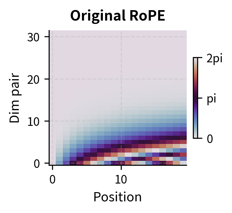
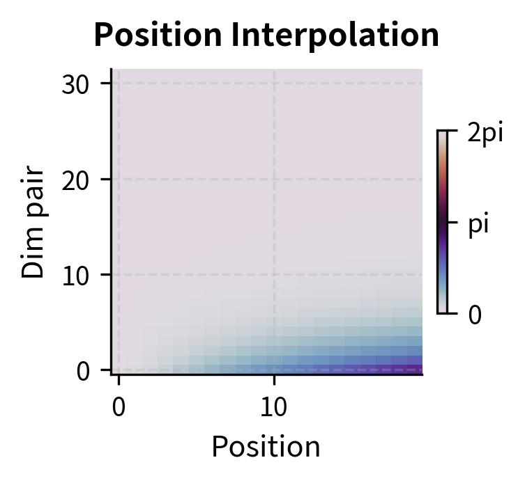
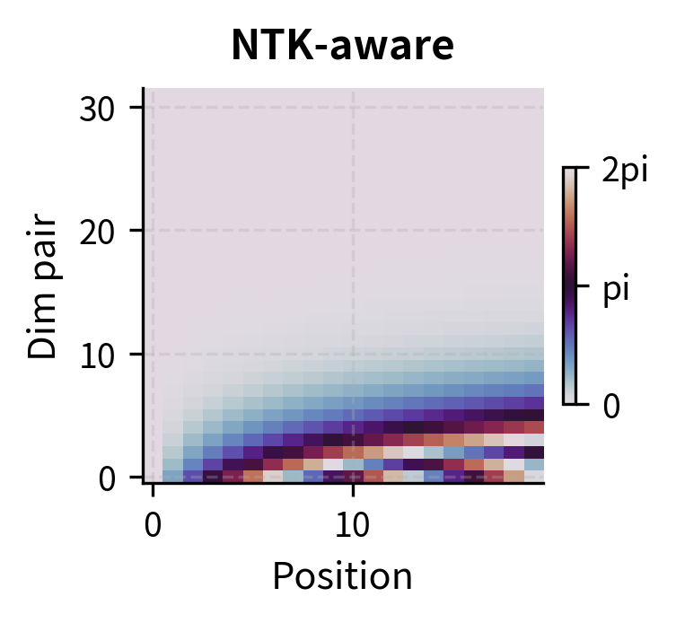
The heatmaps reveal the key difference between methods. In the original (left), the bottom rows (high-frequency dimensions) show rapid color cycling as position increases, while top rows (low-frequency dimensions) change slowly. Position Interpolation (center) uniformly slows down all cycling. NTK-aware scaling (right) preserves the rapid cycling in the bottom rows while slowing only the top rows. This visual confirms that NTK-aware scaling selectively modifies frequencies based on dimension.
Applying RoPE with NTK-aware Scaling
Now that we can compute the frequencies, let's implement the complete RoPE transformation and measure its effect on token distinguishability.
The RoPE Transformation
RoPE works by rotating each pair of embedding dimensions by a position-dependent angle. The rotation angle for position and dimension pair is simply , where is the frequency we computed above:
Measuring Token Distinguishability
The ultimate test of our scaling method is whether adjacent tokens remain distinguishable after rotation. If tokens at positions and become too similar, the model loses its ability to attend precisely to nearby positions.
We'll measure this using cosine similarity between adjacent token embeddings. Lower similarity means more distinguishable tokens:
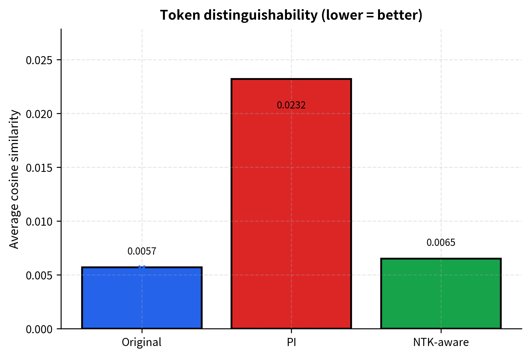
The visualization makes the pattern clear: Position Interpolation significantly increases similarity between adjacent tokens (making them harder to distinguish), while NTK-aware scaling keeps the similarity close to the original. This preservation of token distinguishability is the practical benefit of frequency-dependent scaling.
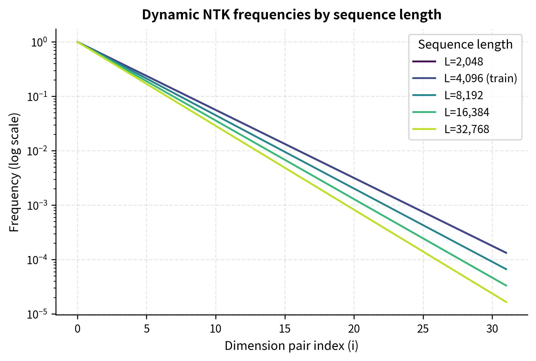
Dynamic NTK Scaling
Static NTK-aware scaling uses a fixed extension factor . But what if the actual sequence length varies? A model configured for 32k tokens shouldn't apply aggressive scaling when processing only 2k tokens. Ideally, the scaling should adapt to the current context: no modification for short sequences, progressive scaling as sequences grow longer.
Dynamic NTK scaling adapts the base in real-time based on the current sequence length:
where:
- : the dynamically computed base, now a function of sequence length
- : the original base (typically 10000)
- : the current sequence length being processed
- : the context length the model was trained with
- : the effective extension factor, computed on-the-fly
- : the same exponent as in static NTK-aware scaling
The formula is identical to static NTK scaling, except that is computed dynamically rather than fixed in advance.
When , the ratio , and we clamp it to 1 (no scaling). When exceeds the training length, scaling kicks in proportionally. A sequence of 8k tokens (2x the training length of 4k) gets ; a sequence of 32k tokens (8x) gets .
The effective base scales smoothly with sequence length. At 32k tokens (8x the training length), the base increases to approximately 87k, matching our earlier static calculation.
Attention Score Analysis
To understand the practical impact, let's examine how attention scores behave under different scaling methods. We'll create synthetic queries and keys at various distances and measure the attention patterns:
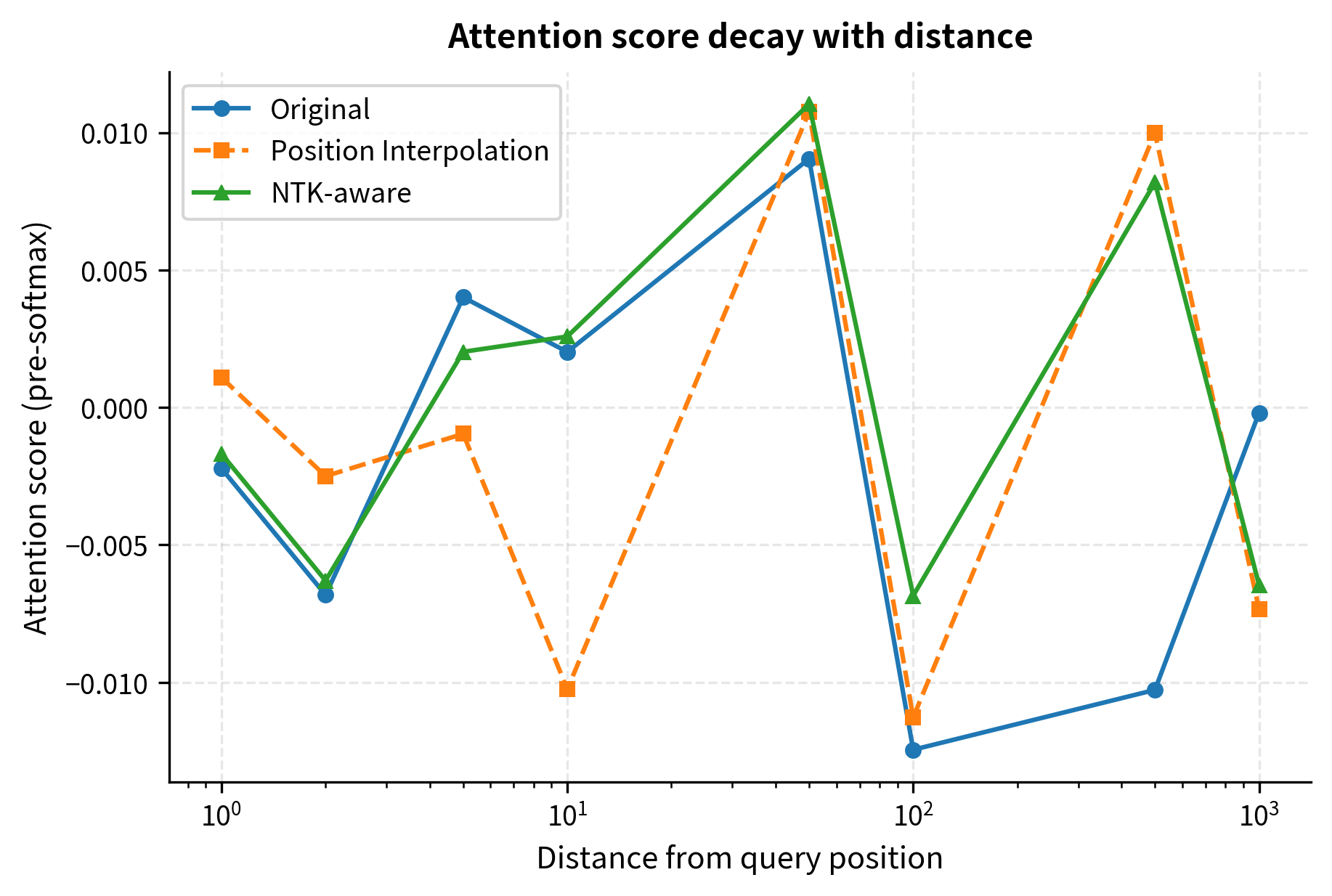
The attention decay pattern reveals a subtle but important distinction. While Position Interpolation flattens the attention curve (making nearby and distant tokens more similar in score), NTK-aware scaling preserves more of the original decay structure, especially at short distances.
Comparing NTK to Position Interpolation
Let's directly compare how well each method preserves the relative position encoding properties:
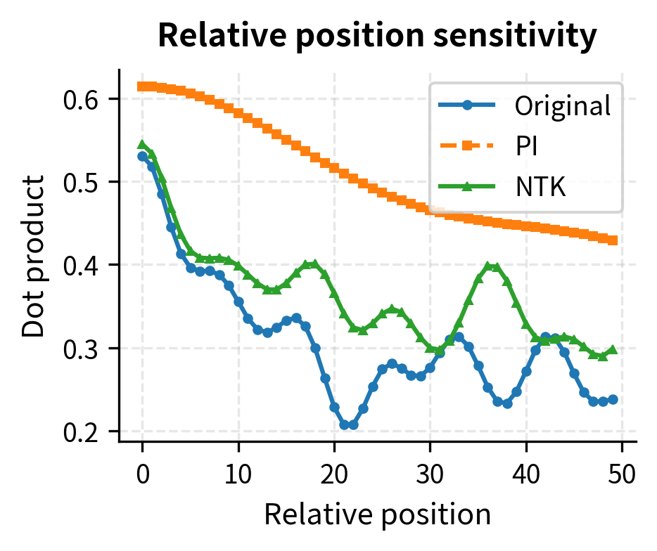
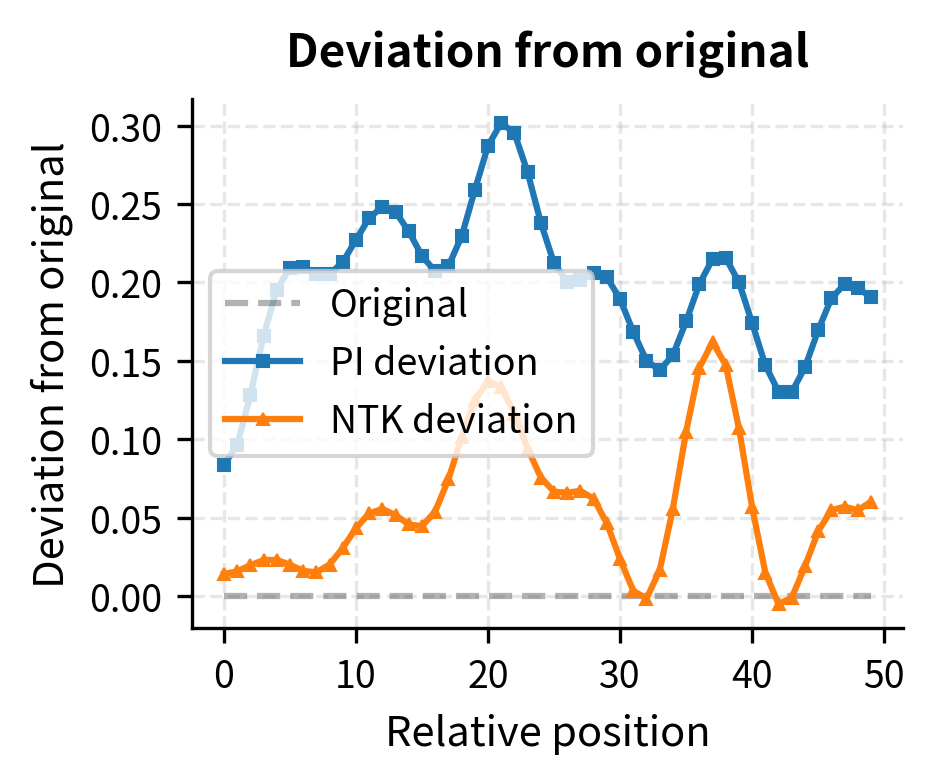
The deviation plot (right) makes the advantage clear: NTK-aware scaling maintains smaller deviations from the original behavior, particularly for small relative positions where local attention patterns matter most.
Interpolation Factor Analysis
An alternative perspective on NTK-aware scaling is to analyze the interpolation factor for each frequency. We can express NTK-aware scaling as a blend between "no interpolation" and "full interpolation":
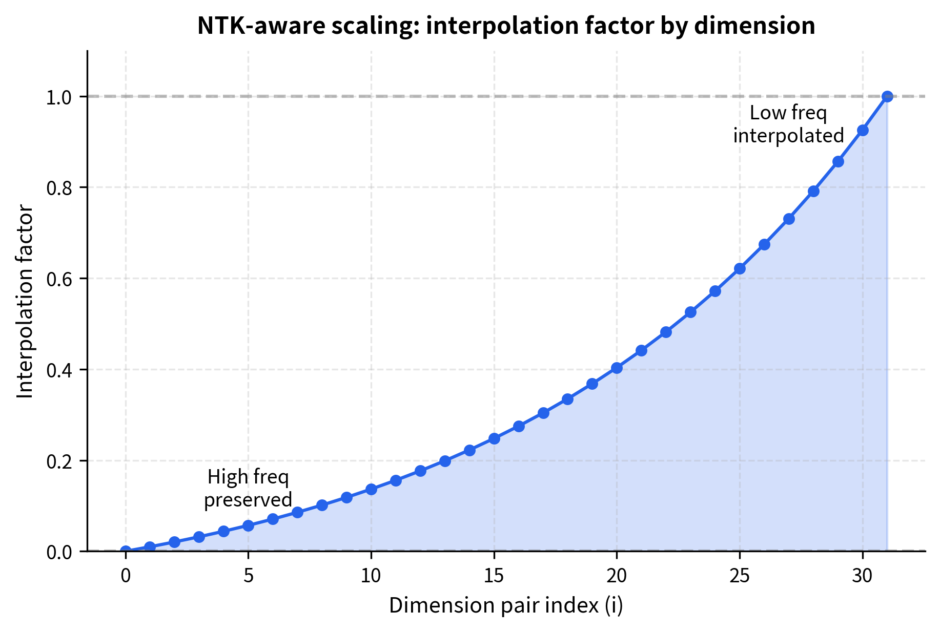
This interpolation perspective provides an intuitive understanding: NTK-aware scaling smoothly transitions from "preserve high frequencies" (interpolation factor near 0) to "fully scale low frequencies" (interpolation factor near 1).
Limitations and Practical Considerations
NTK-aware scaling works better than Position Interpolation, but it comes with its own trade-offs and limitations.
The core tension in context extension is that you cannot perfectly preserve all the properties of the original position encoding while also extending the context window. NTK-aware scaling prioritizes high-frequency preservation at the cost of more aggressive low-frequency compression. For tasks that rely heavily on precise long-range position information, this trade-off may not be ideal. Document retrieval, where finding a specific passage requires accurate global positioning, might suffer compared to summarization tasks where local coherence matters more.
Additionally, NTK-aware scaling, like Position Interpolation, typically requires fine-tuning to achieve optimal performance. While models may work "out of the box" with NTK scaling applied at inference time, the attention patterns learned during training assumed different frequency relationships. Fine-tuning on longer sequences helps the model adapt to the new frequency landscape. The amount of fine-tuning needed is generally comparable to Position Interpolation: a few hundred to a few thousand steps on representative long-context data often suffices.
The choice between static and dynamic NTK scaling depends on deployment constraints. Static scaling is simpler to implement and has deterministic behavior, but requires knowing the maximum context length in advance. Dynamic scaling adapts gracefully to varying sequence lengths but adds computational overhead, as frequencies must be recomputed based on current sequence length. For most applications where sequence lengths are predictable, static scaling is sufficient.
Finally, NTK-aware scaling is specific to RoPE and doesn't transfer to other position encoding schemes. Models using absolute position embeddings, ALiBi, or other mechanisms require different extension strategies. This limits the generality of the approach, though the dominance of RoPE in modern architectures means NTK-aware scaling is broadly applicable.
Key Parameters
When implementing NTK-aware scaling, several parameters control the behavior of the context extension:
-
base (default: 10000): The original RoPE base constant. This value comes from the pretrained model and should match what was used during training. Common values are 10000 (LLaMA, Mistral) or 500000 (some newer models with extended context).
-
scale (s): The context extension factor, computed as target length divided by training length. For example, extending from 4k to 32k tokens gives . Larger values enable longer contexts but increase the distortion from original frequencies.
-
d (embedding dimension): The model's embedding dimension, used in computing the NTK exponent . This is fixed by the model architecture and typically ranges from 64 to 128 for the head dimension in modern transformers.
-
train_length (for dynamic scaling): The context length the model was originally trained with. This serves as the threshold below which no scaling is applied. Using the correct value is critical for dynamic NTK to work properly.
When choosing between static and dynamic scaling, consider your deployment scenario. Static scaling with a fixed is simpler and more predictable, suitable when you know the maximum sequence length in advance. Dynamic scaling adapts to varying inputs but adds computational overhead for recomputing frequencies.
Summary
NTK-aware scaling provides a principled approach to extending context length in RoPE-based models by recognizing that different frequency bands serve different purposes:
-
Key insight: High-frequency components distinguish nearby tokens; low-frequency components capture long-range structure. Uniform scaling damages local precision unnecessarily.
-
The NTK formula: Replace base with , where is the context extension factor. This preserves high frequencies while scaling low frequencies.
-
Frequency-dependent scaling: The effective scaling factor increases from 1 (no change) for the highest frequencies to (full scaling) for the lowest frequencies.
-
Dynamic variant: Adapt the base in real-time based on current sequence length: .
-
Practical benefits: Better preservation of local attention patterns compared to Position Interpolation, especially for tasks requiring precise nearby-token relationships.
NTK-aware scaling improved context extension, but researchers continued seeking even better solutions. In the next chapter, we'll explore YaRN (Yet another RoPE extension method), which builds on NTK-aware principles while adding attention scaling and temperature adjustments for further improvements.
Quiz
Ready to test your understanding? Take this quick quiz to reinforce what you've learned about NTK-aware scaling and context extension in transformer models.

Comments