

Deep dive into LLaMA's core architectural components: pre-norm with RMSNorm for stable training, SwiGLU feed-forward networks for expressive computation, and RoPE for relative position encoding. Learn how these pieces fit together.

This article is part of the free-to-read Language AI Handbook
LLaMA Components
LLaMA's success stems not from revolutionary new ideas, but from carefully selecting and combining the best components available. Each architectural choice, from normalization to positional encoding, was picked based on empirical evidence of what works at scale. The result is a reference design that has influenced virtually every major open-source language model since.
This chapter examines LLaMA's core components in detail: RMSNorm for efficient normalization, SwiGLU for expressive feed-forward computation, and RoPE for relative position encoding. We'll see how these pieces fit together into a coherent architecture, implement a complete LLaMA block from scratch, and understand the design decisions that make LLaMA both powerful and efficient to train.
Pre-Norm with RMSNorm
LLaMA places normalization before each sublayer rather than after. This pre-norm configuration, combined with the simpler RMSNorm instead of LayerNorm, defines the normalization strategy throughout the architecture.
Why Pre-Norm?
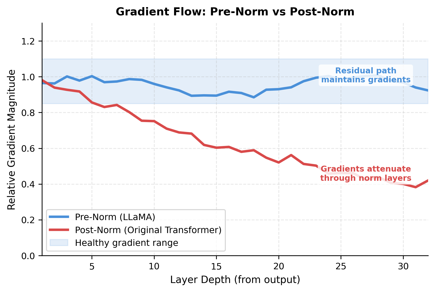
The original transformer used post-norm: normalize after adding the residual connection. This creates a sequence where the residual and sublayer output are summed first, then normalized together. While mathematically elegant, post-norm creates training instabilities in deep networks. Gradients must pass through the normalization layer before reaching the residual path, which can attenuate or distort the gradient signal.
Pre-norm flips this order: normalize the input before the sublayer, then add the unnormalized input via the residual connection. The key benefit is that gradients can flow directly through the residual path without encountering normalization. For a stack of blocks, this means gradients from the output reach early layers with minimal degradation.
The pre-norm equations for a single transformer block are:
where:
- : input to the block with tokens and dimension
- : normalization function (RMSNorm in LLaMA)
- : multi-head self-attention
- : feed-forward network with SwiGLU
- : intermediate representation after the attention sublayer
- : block output
Notice that is added directly to the attention output without normalization, and similarly is added directly to the FFN output. This creates an unimpeded gradient highway through the model.
Why RMSNorm?
To understand RMSNorm, let's first consider what LayerNorm does. LayerNorm performs two operations on each token's representation: centering (subtracting the mean to shift values toward zero) and scaling (dividing by the standard deviation to make the spread consistent). Both operations seem intuitively important for stabilizing neural network training.
RMSNorm challenges this intuition by asking: do we really need both? The answer, surprisingly, is no. Empirical studies found that centering contributes little to training stability, while scaling does the heavy lifting. RMSNorm removes the centering step entirely, normalizing only by the root mean square:
where:
- : input vector (one token's representation)
- : learnable scale parameters
- : small constant for numerical stability (typically )
- : element-wise multiplication
Why does removing centering not hurt performance? The key insight is that the learnable scale parameter gives the network flexibility to adjust the distribution as needed. If centering were truly essential, the model could learn to approximate it through subsequent layers. In practice, models converge just as well without explicit centering.
The practical benefit is speed. RMSNorm saves one reduction operation (computing the mean) and one element-wise operation (subtracting the mean) compared to LayerNorm. These savings seem minor for a single forward pass, but normalization runs at every layer, for every token, at every training step. Over billions of operations, the efficiency gains compound significantly.
Let's implement both normalizations and compare their behavior:
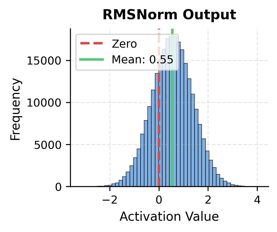
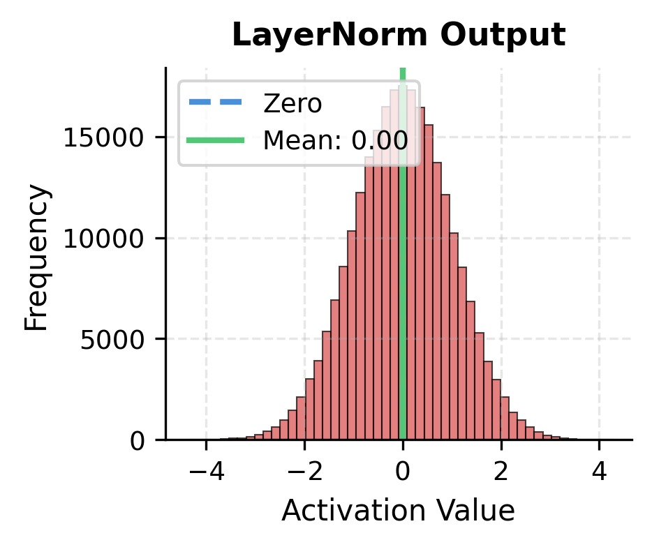
LayerNorm outputs are precisely centered at zero by construction. RMSNorm outputs cluster near zero but aren't exactly centered, since the mean wasn't explicitly subtracted. In practice, this difference rarely matters: the learnable scale parameter can adjust the distribution as needed, and the model learns to work with either normalization scheme.
The SwiGLU Feed-Forward Network
The feed-forward network (FFN) in each transformer block provides the model's primary source of nonlinearity and parameter capacity. While attention handles communication between tokens, the FFN handles computation within each token's representation. This is where the model stores and applies learned knowledge, from factual information to linguistic patterns.
LLaMA uses SwiGLU, a gated variant that has become the standard in modern language models. To understand why SwiGLU works better than simpler alternatives, we'll trace the evolution from basic FFNs to gated architectures, seeing how each improvement addresses specific limitations.
From Standard FFN to Gated Units
The original transformer FFN follows a simple recipe: project each token to a higher dimension, apply a nonlinearity, then project back. This "expand and contract" pattern allows the network to compute complex functions of the input through the nonlinearity in the high-dimensional space:
where:
- : input token representation with dimension
- : first projection, expanding to hidden dimension (typically )
- : second projection, compressing back to model dimension
- : rectified linear unit activation
This architecture works, but it has a limitation: every hidden dimension is processed identically by the ReLU. The network cannot selectively emphasize some features while suppressing others based on the input content.
Gated linear units (GLUs) address this limitation by introducing a learned control mechanism. Instead of applying a fixed activation to all hidden dimensions, a GLU learns which dimensions to activate and which to suppress. It does this by splitting the hidden layer into two parallel paths: one computes a "gate" signal that controls information flow, while the other computes the actual content. These paths are multiplied element-wise:
where:
- : input token representation
- : linear path projection
- : gate path projection
- : output projection
- : sigmoid activation function
- : element-wise (Hadamard) multiplication
The sigmoid-gated path acts as a learned filter, controlling how much of the linear path's information passes through. When is near zero for some hidden dimension, that dimension's contribution is blocked; when near one, it passes through fully.
SwiGLU: Swish-Gated Linear Units
While the sigmoid-gated GLU works well, researchers found an even better gating function: Swish (also called SiLU). The Swish function has an elegant property: it is "self-gating," meaning the input gates itself. Rather than having a separate sigmoid control the gate, Swish multiplies the input by its own sigmoid, creating a smooth, adaptive activation.
SwiGLU applies this insight to the GLU architecture:
where:
- : input token representation with model dimension
- : gate projection matrix
- : up projection matrix (the "linear path")
- : down projection, mapping back to model dimension
- : element-wise multiplication between gate and up projections
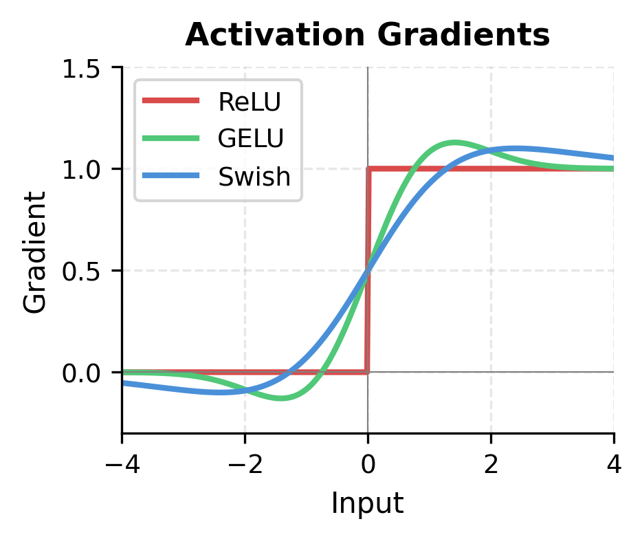
The Swish activation function is defined as:
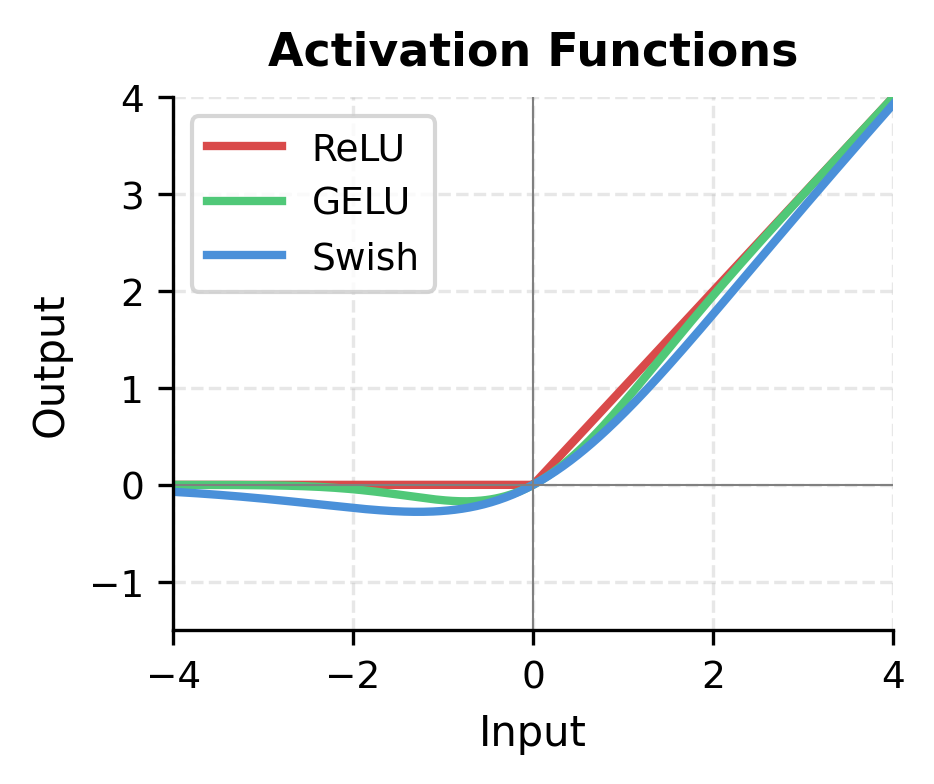
where is the sigmoid function. Swish is smooth everywhere (unlike ReLU's sharp corner at zero) and self-gated: the input is multiplied by its own sigmoid, meaning large positive values pass through nearly unchanged while negative values are attenuated. This combination has been shown to improve training dynamics and final model quality compared to both ReLU and GELU-based FFNs.
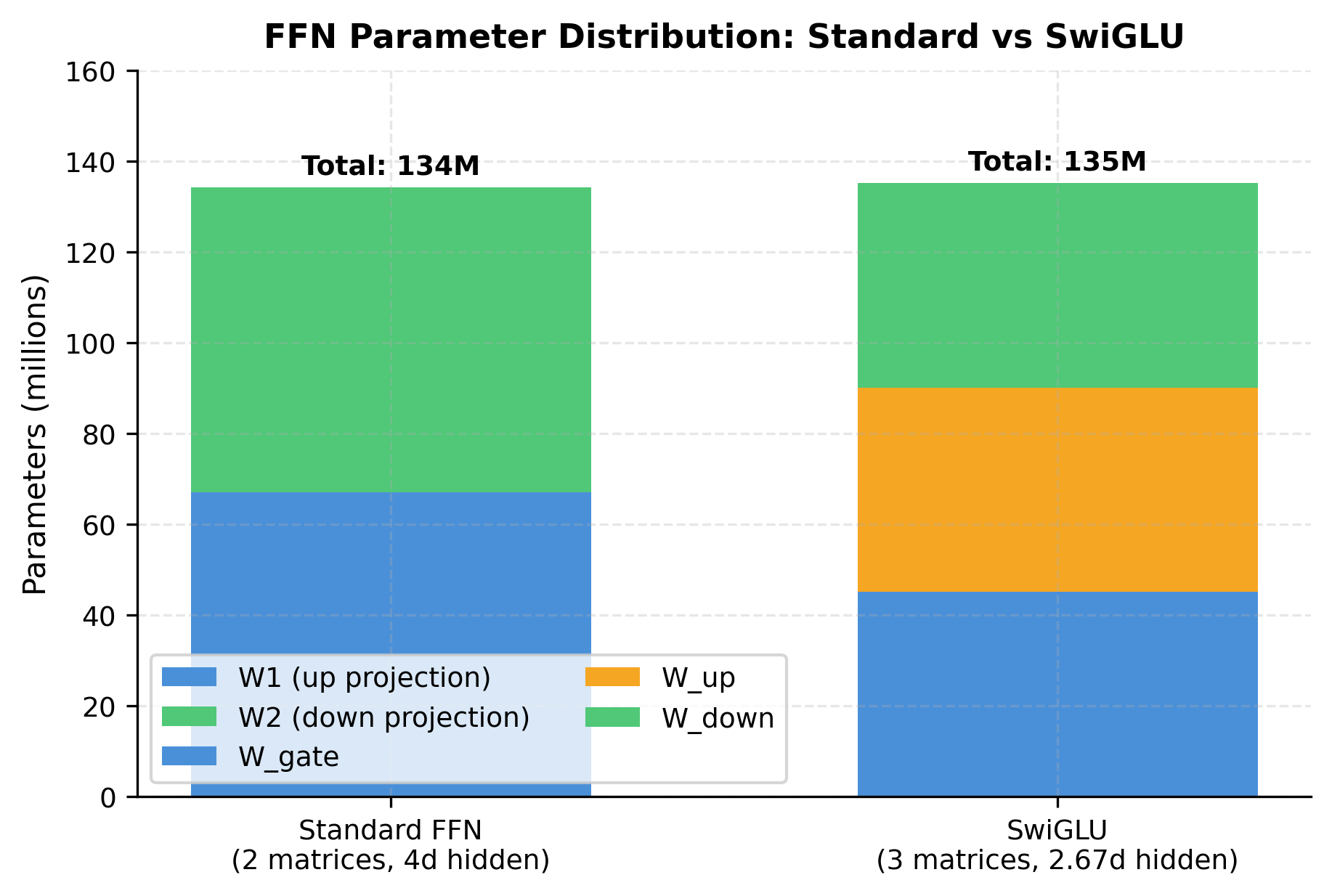
SwiGLU requires three weight matrices (, , ) instead of two (, ). To keep the total parameter count similar, LLaMA reduces the hidden dimension from to approximately . The exact value is often rounded to be divisible by hardware-friendly numbers.
With the theory in place, let's implement SwiGLU and see how the gating mechanism works in practice. We'll first define the Swish activation, then build the complete SwiGLU module:
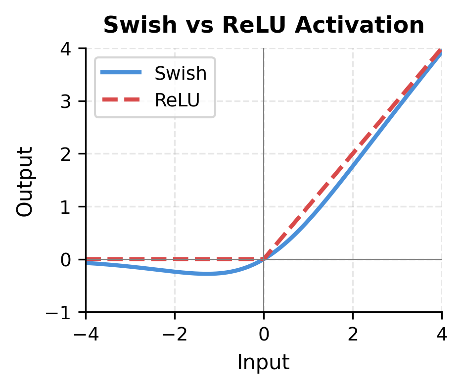
The left plot shows why Swish is preferred over ReLU. Unlike ReLU's hard cutoff at zero, Swish has a smooth curve with non-zero gradients for negative inputs. This helps gradient flow during training, particularly for inputs that happen to fall in negative regions.
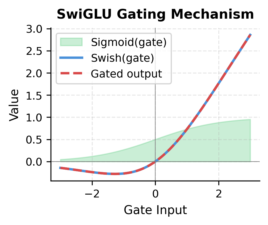
The right plot illustrates gating. When the gate input is negative, the gate output is near zero, blocking information. As the gate input increases, more of the up projection passes through. This learned gating allows the network to selectively process different aspects of the input.
Rotary Position Embedding (RoPE)
Position information in LLaMA comes from Rotary Position Embedding, applied directly to query and key vectors before attention computation. Unlike additive position encodings that modify token embeddings once at the input, RoPE encodes position through rotation at every attention layer.
To understand why LLaMA chose RoPE over simpler alternatives, we need to appreciate a fundamental tension in position encoding: we want the model to understand both where tokens are in a sequence and how far apart they are from each other. Absolute position matters for tasks like "what's the first word?", but relative position matters for language understanding: the relationship between a verb and its subject depends on their distance, not their absolute positions.
Previous approaches added position information to token embeddings at the input layer. This works but has drawbacks: the position signal can degrade through deep networks, and the model must learn to extract relative position from absolute encodings. RoPE solves this elegantly by encoding position in a way that naturally produces relative position information when computing attention scores.
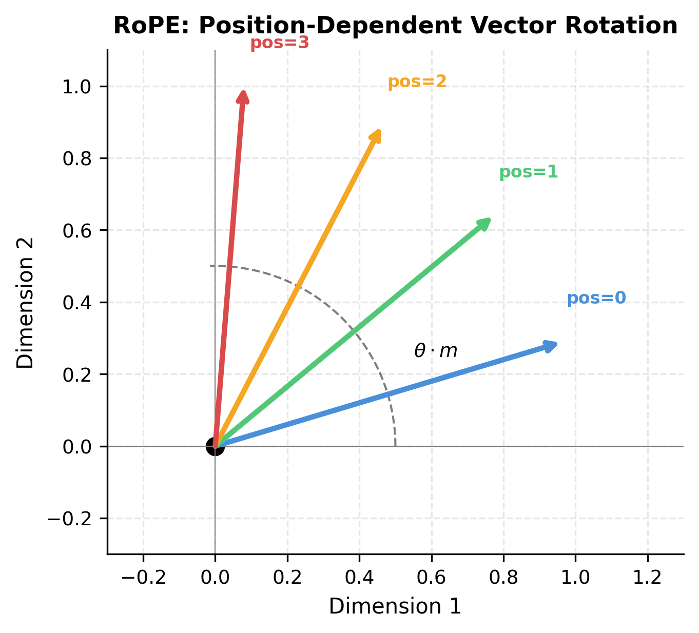
The Rotation Principle
The key insight behind RoPE comes from a beautiful property of rotations. Imagine two arrows (vectors) on a piece of paper. If you rotate both arrows by different amounts and then measure the angle between them, you'll find something remarkable: the angle between them depends only on how much more you rotated one than the other. The absolute rotation amounts don't matter, only their difference.
This is exactly what we want for position encoding. If we rotate the query vector by an amount proportional to its position , and rotate the key vector by an amount proportional to its position , then when we compute their dot product (which measures similarity), the result depends only on the difference . The absolute positions cancel out, leaving pure relative position information.
For a -dimensional embedding, RoPE treats it as independent 2D pairs. Think of each pair as a separate 2D plane where we can apply rotation. Each pair rotates at a different frequency, creating a multi-scale representation: some dimensions capture fine-grained local position differences, while others track global position across the entire sequence.
The rotation angle for dimension pair at position determines how much to rotate that pair. Different dimension pairs rotate at exponentially different rates, following a formula inspired by the original sinusoidal position encodings:
where:
- : the rotation angle (in radians) for dimension pair at sequence position
- : sequence position (0, 1, 2, ...), with for the first token
- : dimension pair index (0, 1, ..., ), grouping dimensions into pairs
- : total embedding dimension (must be even for RoPE)
- : base frequency for dimension pair , which decreases exponentially as increases
- : base constant chosen empirically (same as in sinusoidal position encodings)
The term in the exponent creates the multi-scale effect: when , (fast rotation, one radian per position); when approaches , approaches (very slow rotation). This exponential spacing ensures that the model can distinguish positions at multiple scales simultaneously.
Now we can write the complete RoPE transformation. Given a vector at position , we rotate each pair of dimensions by angle . The rotation uses the standard 2D rotation formula you might remember from linear algebra: to rotate a point by angle , you compute . Applying this to all dimension pairs gives:
where:
- : the input query or key vector
- : the first dimension pair, rotated by angle
- : the second dimension pair, rotated by angle
- : rotation components for pair at position
Each pair is rotated independently using the standard 2D rotation formulas: and . This preserves the vector's magnitude while encoding position through angle. The preservation of magnitude is crucial: we're adding position information without distorting the semantic content of the embedding.
In practice, we don't need to construct explicit rotation matrices. Instead, we can compute the rotations efficiently using element-wise operations. The key observation is that for each dimension pair, we just need to:
- Compute the angle for that pair at position
- Calculate and of the angle
- Apply the rotation formula to the pair
Let's implement this step by step:
Let's visualize how RoPE creates position-dependent rotations across different frequencies:
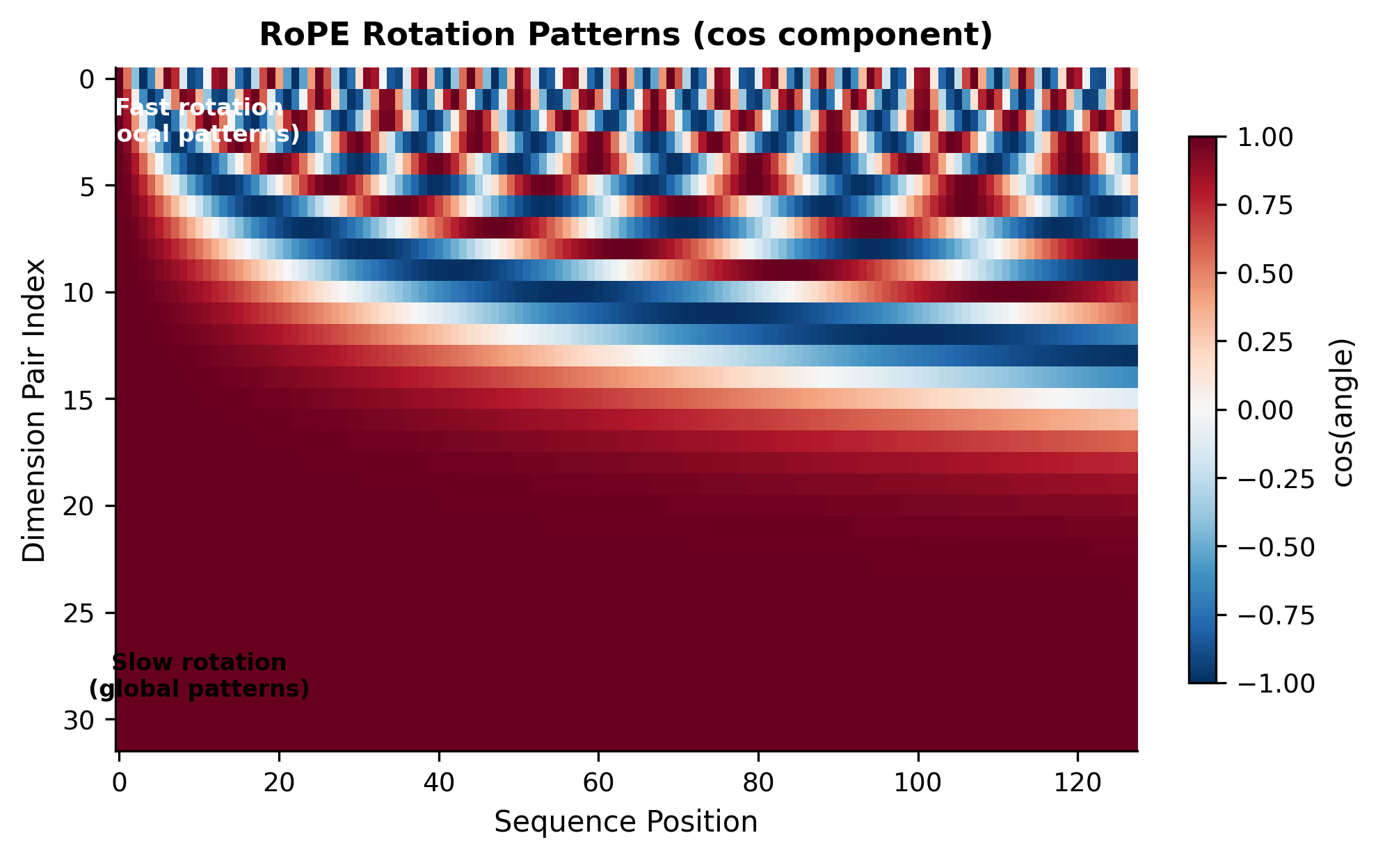
The heatmap reveals RoPE's multi-scale nature. Dimension pairs near the top (low index) oscillate rapidly: they complete many cycles across the sequence and can distinguish nearby positions precisely. Dimension pairs near the bottom (high index) change slowly: they differentiate positions that are far apart. Together, they create a rich position encoding that works at all scales.
RoPE in Attention
RoPE is applied to query and key vectors before computing attention scores. Critically, it is not applied to values. To understand why, consider what happens when we compute the attention score between a query at position and a key at position .
Without RoPE, the dot product between query and key gives:
With RoPE, both vectors are rotated before the dot product. For a single 2D pair, if we rotate by angle and by angle , the dot product becomes:
where:
- : query and key vectors for a single dimension pair
- : the 2D rotation matrix
- : the transpose of a rotation matrix is its inverse (rotation by the negative angle)
- : rotation angles at positions and respectively
The key insight: . The absolute positions and cancel out, leaving only their difference . This is how RoPE encodes relative position: the attention score between two positions depends only on how far apart they are, not where they appear in the sequence.
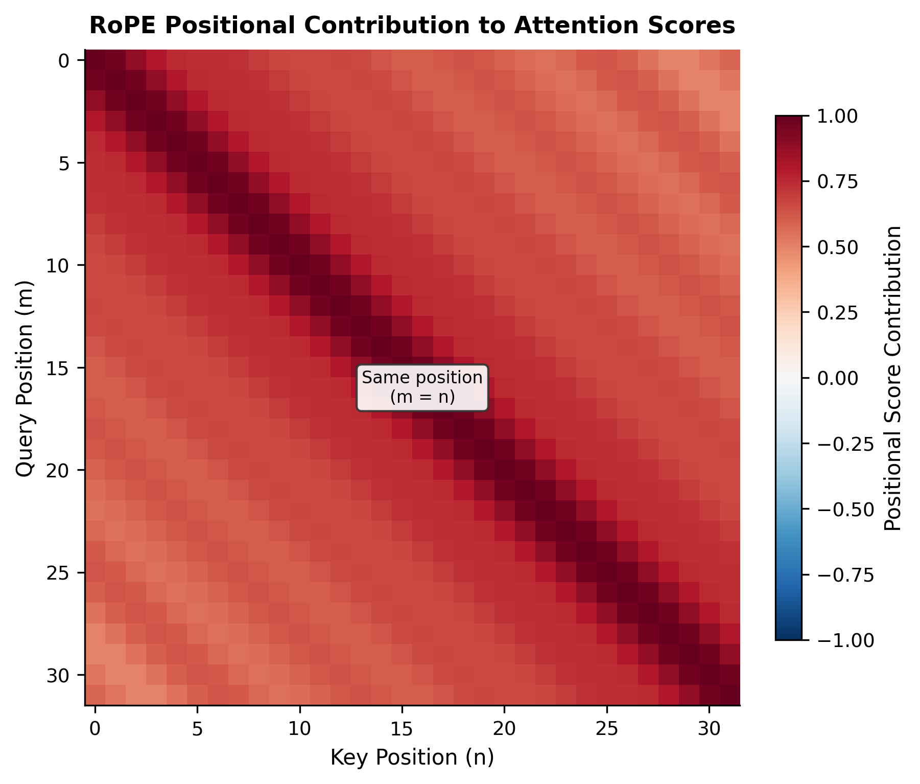
Values don't participate in this relative position mechanism; they simply carry the information to be aggregated based on the position-aware attention weights.
Component Interactions
Understanding each component in isolation is valuable, but the real insight comes from seeing how they interact. In LLaMA, the components form a carefully orchestrated pipeline where each element's design choices complement the others.
The Information Flow
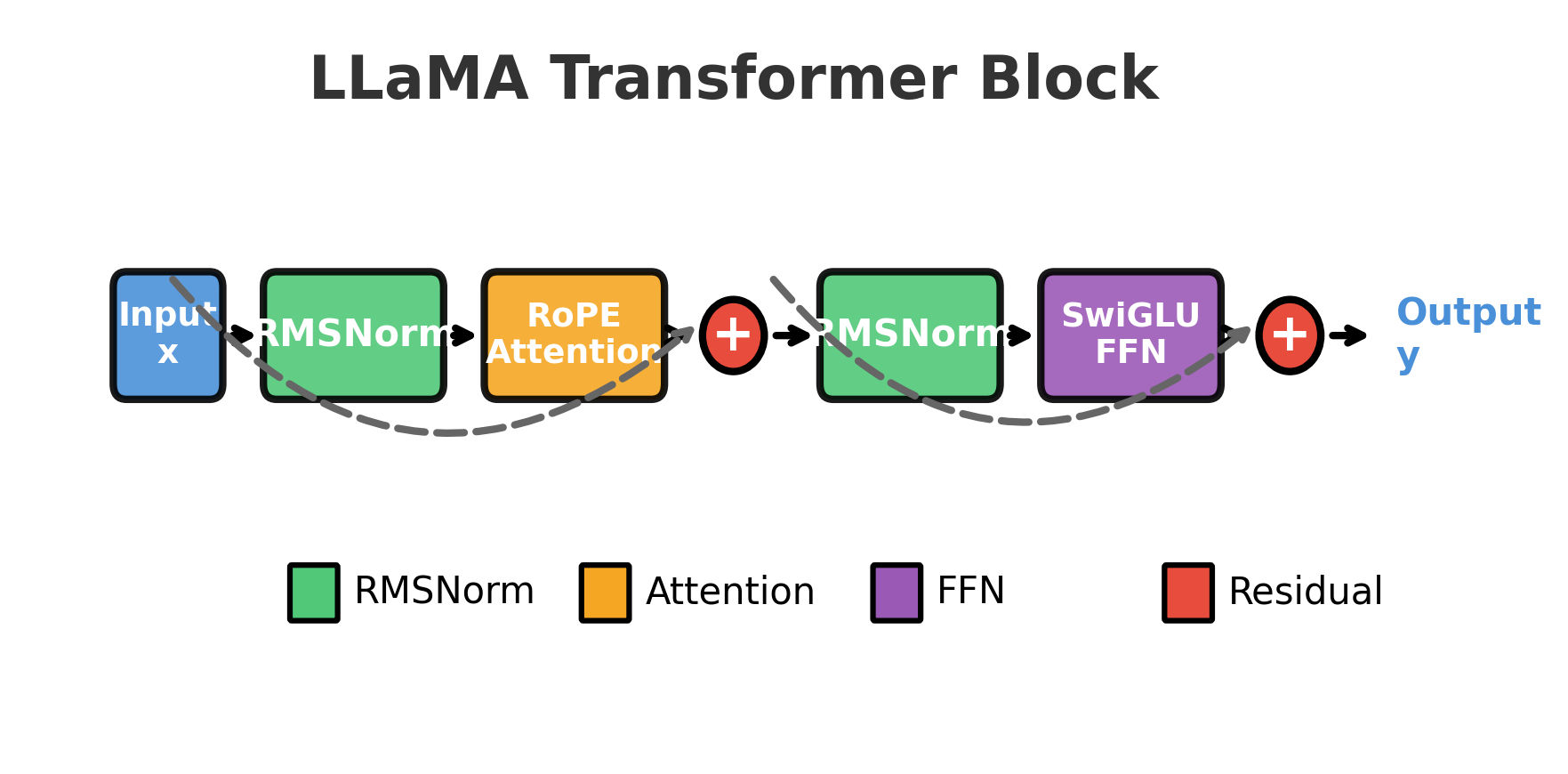
A single LLaMA block processes input through the following sequence:
- Pre-attention RMSNorm: Stabilizes activations before attention
- RoPE-enhanced attention: Mixes information across positions with relative position awareness
- Residual connection: Adds attention output to original input
- Pre-FFN RMSNorm: Stabilizes activations before the feed-forward network
- SwiGLU FFN: Transforms each position independently through gated nonlinearity
- Residual connection: Adds FFN output to post-attention representation
Let's visualize this flow:
Why This Combination Works
The components weren't selected arbitrarily. Each choice addresses specific challenges in training and inference:
RMSNorm + Pre-Norm provides stable gradients for deep networks. The pre-norm configuration creates direct gradient paths through residuals, while RMSNorm's efficiency matters when normalization runs at every layer.
RoPE enables long-context extension through interpolation. Since RoPE applies rotation at inference time rather than fixed position embeddings, the model can extrapolate to longer sequences than seen during training (with appropriate scaling techniques).
SwiGLU provides expressive nonlinearity without the dead neuron problem of ReLU. The gating mechanism learns to selectively process information, and the smooth Swish activation ensures gradients flow through all neurons.
Together, these choices create an architecture that trains stably at scale, infers efficiently, and generalizes well to new contexts.
Implementation: A Complete LLaMA Block
Let's assemble all components into a complete LLaMA transformer block:
Let's test our implementation with a small example:
The output maintains the same shape as the input, as expected for a transformer block. The mean and standard deviation of the output remain in a reasonable range, demonstrating that RMSNorm successfully stabilizes activations. Without normalization, activations could grow or shrink exponentially through many layers, making training unstable. The fact that output statistics stay close to the input statistics is a good sign that the block is well-behaved.
Stacking Blocks into a Model
A complete LLaMA model stacks many blocks, adds embeddings at the input, and applies a final normalization before the output projection:
This simplified model demonstrates the complete LLaMA architecture. The output logits have shape (8, 1000), meaning for each of the 8 input tokens, we get a probability distribution over the 1000-word vocabulary. The top predictions for the next token show varying logit values, which would become probabilities after applying softmax. Since the model uses random weights, these predictions are meaningless, but the structure shows how a trained model would generate text token by token.
Note the absence of learned position embeddings at the input, since RoPE encodes position directly in the attention mechanism. This is a key architectural difference from GPT-style models, where position embeddings are added to token embeddings at the input layer.
Parameter Distribution
Understanding where parameters reside helps explain why certain design choices matter. Let's analyze the parameter distribution in a LLaMA block:
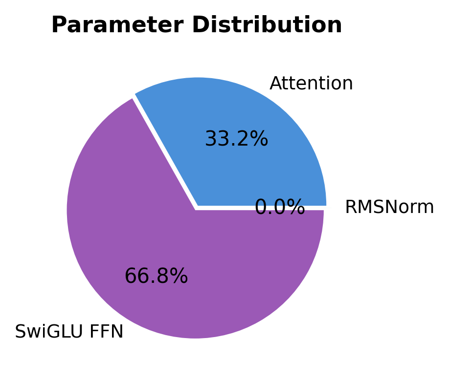
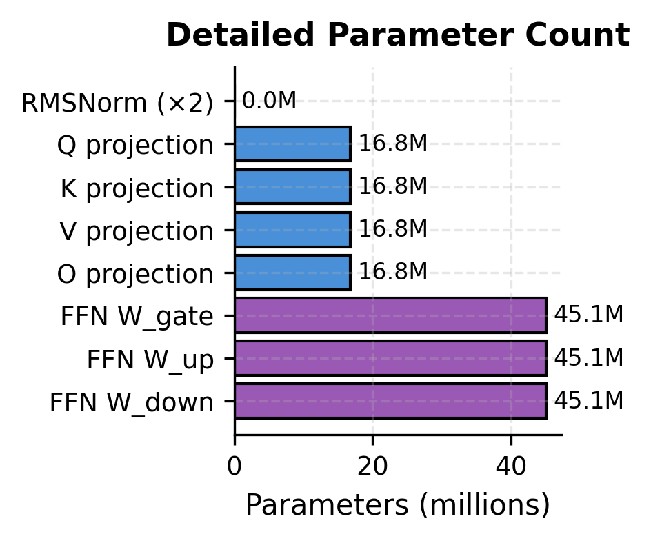
The FFN dominates parameter count despite SwiGLU's efficiency improvements. This is because:
- The hidden dimension is large (about 2.7x )
- SwiGLU uses three matrices instead of two
However, this investment pays off. The FFN provides the model's primary capacity for storing learned patterns and facts. The attention mechanism, while containing fewer parameters, handles the crucial task of routing information between positions.
Limitations and Trade-offs
LLaMA's component choices, while effective, come with trade-offs worth understanding.
RMSNorm's simplification has theoretical gaps. By removing mean centering, RMSNorm assumes that the mean of activations is either unimportant or learnable through other means. For most language modeling tasks, this assumption holds. However, tasks requiring precise tracking of activation magnitudes across layers might benefit from full LayerNorm. The empirical success of RMSNorm suggests these cases are rare in practice.
SwiGLU's parameter overhead. The three-matrix design of SwiGLU means that for a fixed parameter budget, the hidden dimension must be smaller than with a two-matrix FFN. This trades width for gating capability. Whether this is optimal depends on the model scale: very large models might benefit from simpler, wider FFNs, while smaller models gain from SwiGLU's expressiveness.
RoPE's computational cost. Applying rotations at every attention layer adds overhead compared to one-time positional embeddings. For short sequences, this overhead is negligible. For very long contexts, the repeated rotation computation becomes more significant. Modern implementations optimize this through precomputation and efficient kernels.
The pre-norm stability assumption. Pre-norm works because it assumes the residual stream is the "main highway" for information. This can make it harder for deep layers to fundamentally transform representations, since they always add to the existing stream. Some architectures experiment with adaptive residual weights to address this.
Despite these limitations, LLaMA's component choices represent a well-tuned balance. The architecture trains stably, infers efficiently, and achieves strong performance across diverse tasks. The design decisions have proven robust across model scales from 7B to 405B parameters, validating the choices made at the component level.
Key Parameters
When implementing or configuring LLaMA-style models, several parameters significantly impact model behavior and performance:
Model Dimension (d_model)
- Controls the width of the model and the size of token representations
- Typical values: 4096 (7B), 5120 (13B), 8192 (70B)
- Larger values increase capacity but also memory and compute requirements
- Must be divisible by the number of attention heads
Number of Attention Heads (n_heads)
- Determines how many parallel attention patterns the model can learn
- Typical values: 32 (7B), 40 (13B), 64 (70B)
- More heads allow diverse attention patterns but increase complexity
- Head dimension (
d_model / n_heads) should typically be 64-128 for efficiency
FFN Hidden Dimension (d_ff)
- Sets the expansion factor in the feed-forward network
- For SwiGLU, typically (compared to for standard FFN)
- Often rounded to be divisible by 256 or 1024 for hardware efficiency
- Example: LLaMA 7B uses 11008 (vs. naive 10923 from )
RoPE Base (rope_base)
- Controls the frequency range of position encodings
- Default: 10000 (inherited from original sinusoidal encodings)
- Higher values extend effective context length but may reduce precision for nearby positions
- Some models use 500000 or higher for very long contexts
RMSNorm Epsilon (eps)
- Small constant for numerical stability in normalization
- Typical value: or
- Rarely needs tuning unless encountering numerical issues
Number of Layers (n_layers)
- Determines model depth
- Typical values: 32 (7B), 40 (13B), 80 (70B)
- More layers increase capacity and sequential dependency but slow inference
- Deeper models require more careful initialization and learning rate tuning
Summary
LLaMA's architecture demonstrates how careful component selection creates a coherent, efficient design. The key components and their roles:
-
Pre-norm with RMSNorm provides stable gradient flow through deep networks. Normalization before each sublayer creates direct residual paths, while RMSNorm's efficiency (skipping mean centering) reduces computational overhead without sacrificing quality.
-
SwiGLU FFN delivers expressive nonlinearity through gated linear units. The Swish activation provides smooth gradients, and the gating mechanism learns to selectively process information. The trade-off is three weight matrices instead of two, compensated by a reduced hidden dimension.
-
RoPE encodes relative position through rotation. Applied to queries and keys at every layer, it enables position-aware attention without additive embeddings. The multi-frequency design captures both local and global position information.
-
Component interaction matters as much as individual choices. Pre-norm + residuals create gradient highways. RoPE enables context extension through interpolation. SwiGLU provides the nonlinearity that attention alone cannot.
The complete LLaMA block follows a consistent pattern: normalize, transform, add residual. This pattern repeats for attention and FFN sublayers, creating a modular, stackable unit that scales to hundreds of billions of parameters.
Understanding these components prepares you for the next chapters, where we'll examine variations like grouped-query attention that further optimize the LLaMA design for inference efficiency.

Comments