YaRN: Extending Context Length

Extending context length in large language models has become one of the most practically important research directions in the field. Models trained on sequences of 2,048 or 4,096 tokens struggle when asked to process documents spanning tens of thousands of positions: a legal contract, a scientific paper, an entire codebase, or an hour-long meeting transcript. The naive solution of simply feeding in longer sequences fails because the model was never shown those position indices during training. Its position encodings, like any learned representation, degrade when pushed beyond their training distribution.

Position Interpolation offered one solution: scale down position indices to fit within the trained range. If a model was trained on positions 0 through 2047, and you want to process a 8,192-token document, divide every position index by 4. Suddenly every position index is back in familiar territory. The idea is clever and works surprisingly well, but it introduces a problem: compressing positions uniformly blurs the fine-grained distinctions that high-frequency components encode. Tokens that were one step apart now appear (in the rotated embedding space) as if they are one quarter of a step apart.

NTK-aware scaling improved upon this by treating the frequency spectrum as a whole rather than scaling positions directly. Instead of shrinking positions, it modifies the base frequency of the RoPE formula, which pushes low-frequency components to cover longer distances while leaving high-frequency components comparatively intact. This preserves the model's ability to distinguish nearby tokens while extending the range of distant-position encoding. For moderate extensions (2x to 4x), NTK-aware scaling works well. But as the extension factor grows, even this more sophisticated approach begins to degrade, because it still does not account for a second, more subtle problem: the effect of position encoding changes on attention score distributions.

YaRN, which stands for "Yet another RoPE extensioN," addresses limitations in both approaches. The key insight is that extending context length does not just require fixing position encodings. It also requires compensating for a subtle but significant change in attention score distributions. When we stretch positions across longer sequences, the entropy of attention distributions shifts in ways that degrade model behavior. A model that learned to focus sharply on specific positions during training will find itself attending more diffusely after context extension, because the geometric compression of positions makes all keys look more similar to every query. YaRN tackles this through a combination of targeted frequency interpolation and an attention temperature correction.

Think of YaRN as a two-part repair kit for extended models. The first part (the ramp function) is a surgeon's tool: it operates on different frequency bands of the rotation spectrum independently, leaving untouched what doesn't need fixing while carefully adjusting what does. The second part (temperature scaling) is a lens: it sharpens the blur that the first operation inevitably introduces into attention distributions. Neither component alone is sufficient. Together, they enable models to maintain quality at context lengths 16x or 32x beyond their training distribution.

This chapter develops YaRN from its motivation through its complete formulation. We'll see why existing methods fall short at large extension factors, derive the attention scaling mechanism step by step, and implement YaRN from scratch. By the end, you'll understand how YaRN works and why each design choice matters when applying it to real models.

Before diving into YaRN, let's understand precisely why Position Interpolation and NTK-aware scaling leave room for improvement. Both methods successfully enable RoPE-based models to process longer sequences, but they introduce subtle distortions that accumulate as the extension factor increases. Understanding these distortions motivates every design choice in YaRN.

Rotary Position Embedding (RoPE) encodes position by rotating token embeddings in the complex plane. Each pair of embedding dimensions is assigned a rotation frequency $\theta_i$, ranging from high frequencies (rapid rotation, distinguishing nearby tokens) to low frequencies (slow rotation, distinguishing distant tokens). The key property of RoPE is that the dot product between a query at position $m$ and a key at position $n$ depends only on their relative offset $m - n$. This is what gives transformer models their relative position sensitivity.

Position Interpolation works by scaling all position indices by a factor $s$: a position $m$ becomes $m/s$. This keeps all positions within the trained range, but it compresses the entire frequency spectrum uniformly. High-frequency dimensions that previously distinguished positions 1 apart now need to distinguish positions $s$ apart after compression. The model loses fine-grained position discrimination in all frequency bands simultaneously. Think of it as zooming out on a photograph: every detail shrinks by the same factor, and fine details become indistinguishable. For small extension factors (1.5x or 2x), the blurring is tolerable. For larger factors, the high-frequency bands lose so much precision that nearby tokens begin to look indistinguishable.

NTK-aware scaling addresses this by adjusting the base frequency rather than scaling positions directly. This preserves high-frequency components while stretching low-frequency ones. The approach works well for moderate extensions (2x to 4x), but at larger factors, even NTK-aware scaling begins to degrade. The root issue is that NTK-aware scaling still applies the same mathematical transformation uniformly across all dimension pairs, just with a different parameterization. Some dimension pairs benefit from modification; others would be better left alone. Neither PI nor NTK provides the dimension-specific control that optimal extension requires.

There is also a second limitation that both methods share: neither accounts for the entropy change that interpolation introduces into attention distributions. Modifying position encodings changes how similar queries look to keys across different positions. When positions appear compressed, all keys look more similar to every query, and the softmax over attention scores becomes flatter. This entropy increase is not a feature. It is a side effect that degrades the model's ability to focus on specific relevant tokens. YaRN is the first method to address this problem explicitly and correct for it with a principled formula.

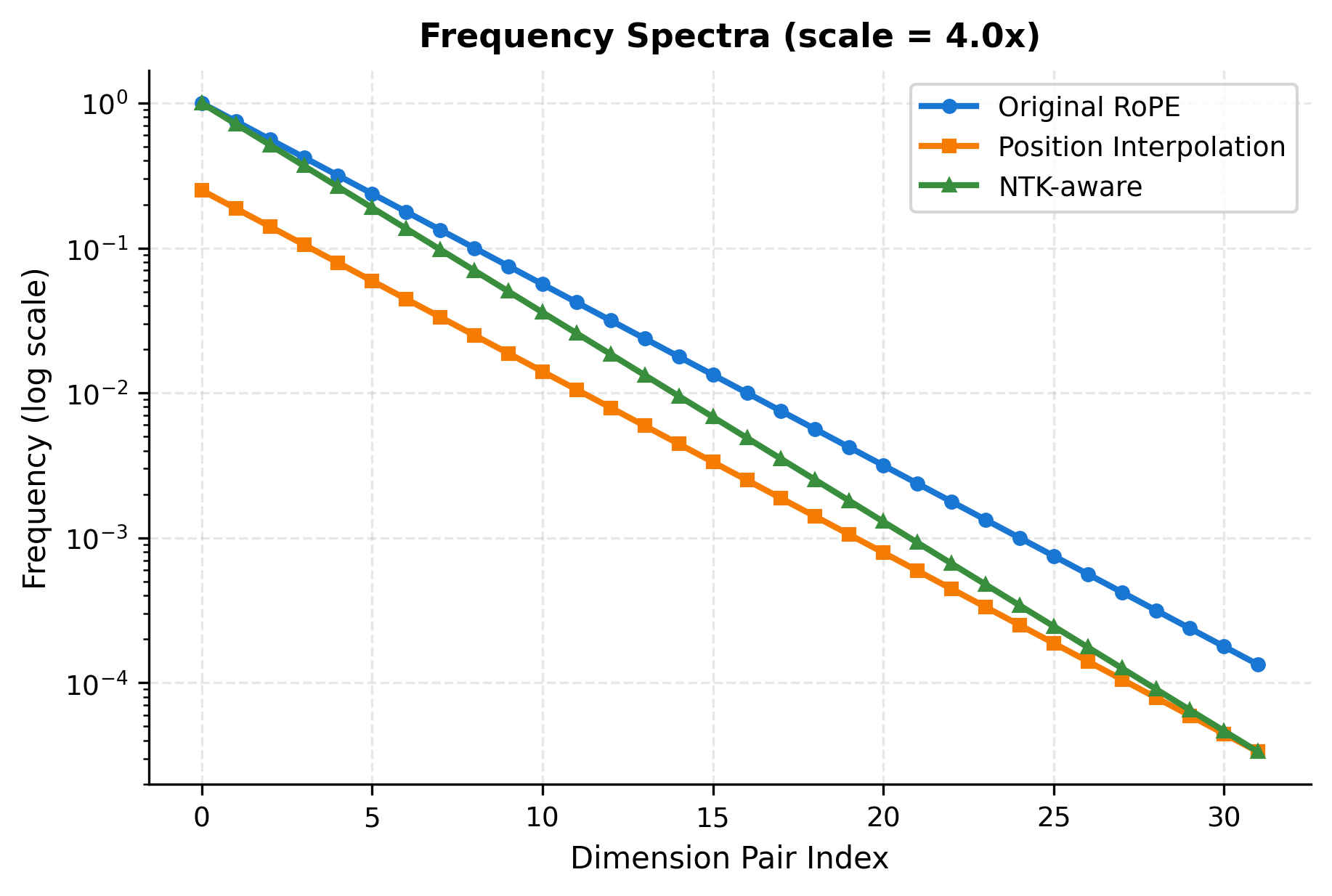
The visualization reveals a fundamental trade-off. Position Interpolation maintains the relative spacing between frequencies (the lines are parallel on a log scale) but shifts everything down uniformly. NTK-aware scaling bends the curve, keeping high frequencies close to original while aggressively stretching low frequencies. Neither approach is optimal across all dimension pairs, because they apply a global transformation where a dimension-specific one is needed.

Beyond frequency adjustments, there is a more subtle issue that neither PI nor NTK-aware scaling addresses: attention entropy shifts. When we modify RoPE frequencies, we change the distribution of attention scores in ways that affect model behavior in a systematic and problematic direction. Understanding this problem requires thinking carefully about what attention score distributions represent and why their entropy matters.

Recall that attention scores are computed as the scaled dot product between query and key vectors. These scores are then passed through a softmax to produce attention weights that sum to one. The resulting distribution tells the model how much to focus on each key position. A low-entropy distribution is sharply peaked, meaning the model strongly attends to one or a few positions. A high-entropy distribution is flat, meaning the model spreads its attention diffusely. During training, models learn attention patterns calibrated to the natural entropy of the position encoding scheme they were trained with. If you change that entropy, you change the effective behavior of every attention head in every layer.

Recall that attention scores are computed as the scaled dot product between query and key vectors:

where:

• $\text{score}(m, n)$: the attention score between a query at position $m$ and a key at position $n$
• $\mathbf{q}_m$: the RoPE-rotated query vector at sequence position $m$
• $\mathbf{k}_n$: the RoPE-rotated key vector at sequence position $n$
• $d_k$: the dimension of the key vectors, used for scaling to prevent dot products from growing too large in magnitude
• $\mathbf{q}_m^\top \mathbf{k}_n$: the dot product between query and key, measuring their geometric similarity after rotation

When we interpolate positions, the effective distances between tokens change in the rotated embedding space. Positions that were far apart now appear closer in that space. This compression happens because we have slowed down the rotation rates, so two tokens that used to be separated by many radians of rotation are now separated by fewer. This reduction in angular separation increases the cosine similarity between their rotated representations, which increases the dot product, which compresses the range of attention scores.

Higher score compression means higher entropy: the model attends more diffusely rather than focusing on specific positions. The softmax function is particularly sensitive to the scale of its inputs. When inputs are spread out, the largest values dominate strongly and the output is peaked. When inputs are compressed, the softmax output becomes more uniform. This is the same phenomenon that temperature scaling in language model generation exploits, and it is exactly what YaRN needs to counteract.

The key insight is that this entropy problem is not fixed by improving the frequency adjustment alone. Even a perfect frequency adjustment that places every dimension pair's rotation frequency exactly where we would want it will still change the geometry of the rotated embedding space. The act of enabling longer contexts changes the statistics of attention, and YaRN compensates with a direct correction to attention scores.

Let's quantify this effect by computing attention entropy under different interpolation schemes:

The entropy values reveal the effect of position interpolation on attention patterns. Both PI and NTK-aware scaling increase entropy compared to the original RoPE. While the differences might seem modest in absolute terms, they compound across layers and affect the model's ability to retrieve and aggregate information from specific positions. A model that learned to perform sharp, focused retrieval with original RoPE will now perform softer, more diffuse retrieval after extension, degrading quality on tasks that require pinpoint attention. YaRN addresses this by introducing an attention temperature correction that pushes the entropy back toward the original distribution.

YaRN combines two complementary mechanisms to enable high-quality context extension. Neither mechanism is sufficient on its own: the frequency adjustment alone does not fix the entropy problem, and the temperature correction alone does not fix the frequency distortion. But together, they address both sources of degradation in a way that is both principled and computationally lightweight.

The first mechanism is ramp-based frequency interpolation. Rather than treating all dimension pairs equally (like PI) or smoothly transitioning across all pairs using a single global parameter (like NTK), YaRN uses a ramp function that applies no interpolation to high-frequency pairs, full interpolation to low-frequency pairs, and a smooth linear transition in between. The threshold between "needs interpolation" and "does not need interpolation" is based on whether the pair's rotation wavelength fits within the original training context. This makes the interpolation decision interpretable and motivated by the actual frequency behavior of each dimension.

The second mechanism is attention temperature scaling. YaRN introduces a scaling factor $\sqrt{t}$ applied to attention scores before softmax, where $t \geq 1$ is computed from the extension factor $s$ via an empirically derived formula. This scaling increases the spread of attention scores, counteracting the compression effect of interpolation. When $s = 1$ (no extension), $t = 1$ and no scaling is applied, preserving the original behavior exactly.

The combined approach modifies both the rotation frequencies and the attention computation. For frequencies, YaRN applies a dimension-specific adjustment. The core idea is to compute a modified frequency $\theta'_i$ for each dimension pair $i$:

where:

• $\theta'_i$: the adjusted frequency for dimension pair $i$ after YaRN modification
• $\theta_i$: the original RoPE frequency for dimension pair $i$, computed as $1/10000^{2i/d}$
• $\gamma(r_i)$: the interpolation factor, a value between $1/s$ and $1$ that depends on the wavelength ratio for this dimension
• $r_i = \lambda_i / L$: the wavelength-to-context ratio for dimension pair $i$, comparing this pair's rotation period to the training context length
• $\lambda_i$: the wavelength for dimension pair $i$, measuring how many sequence positions correspond to one full rotation
• $L$: the original training context length (e.g., 2048 or 4096 tokens)

Why does this formula make sense? Notice that when $\gamma(r_i) = 1$, the adjusted frequency equals the original frequency: no change. When $\gamma(r_i) = 1/s$, the adjusted frequency is scaled down by exactly the extension factor, which is equivalent to Position Interpolation applied to just this dimension. The ramp function interpolates between these extremes based on how much this particular frequency needs correction.

For attention scores, YaRN introduces a temperature correction:

where:

• $\text{score}'(m, n)$: the temperature-adjusted attention score between positions $m$ and $n$
• $\sqrt{t}$: the temperature scaling factor, where $t > 1$ increases score magnitude and sharpens the attention distribution
• $t$: the temperature parameter, computed from the extension factor $s$ via $t = 0.1 \ln(s) + 1$
• $\mathbf{q}_m$, $\mathbf{k}_n$: the YaRN-rotated query and key vectors at positions $m$ and $n$
• $d_k$: the dimension of key vectors, used for the standard $\sqrt{d_k}$ scaling

The scaling factor $\sqrt{t}$ appears before the softmax, not after. Multiplying pre-softmax scores by a constant $c$ sharpens the distribution (for $c > 1$) in the same way that reducing temperature does in generative sampling. YaRN uses this mechanism to counteract the entropy increase from frequency interpolation.

Let's develop each component in detail.

To understand why some dimension pairs need interpolation while others don't, we need to think about rotation in terms of wavelength rather than frequency. While frequency tells us how fast something rotates (radians per position), wavelength tells us how far we must travel for one complete cycle (positions per full rotation). Wavelength provides a more intuitive picture because we can directly compare it to the context length: if a wavelength is shorter than the context, the pair completes multiple full rotations during training; if longer, it completes only a fraction of one rotation.

Think of a dimension pair's rotation as a clock hand sweeping around a circle. A high-frequency pair is like a second hand: it completes many full rotations in the span of the training context. Every possible angle has been visited many times. The model knows how to use all parts of the rotation cycle to distinguish positions. A low-frequency pair is like an hour hand: it moves very slowly, covering only a small arc during training. The model has only seen a fraction of the rotation cycle, and it uses that small arc to encode position. If we extend the context beyond training, the second-hand pair has no problem: it just keeps spinning. But the hour-hand pair is now asked to cover territory it has never visited, and extrapolation fails.

The wavelength $\lambda_i$ of dimension pair $i$ is the inverse of the frequency, scaled by $2\pi$:

where:

• $\lambda_i$: the wavelength (in positions) for dimension pair $i$, representing how many sequence positions correspond to one complete rotation cycle
• $\theta_i = 1/10000^{2i/d}$: the base frequency for dimension pair $i$, measured in radians per position
• $d$: the total embedding dimension (must be even, since RoPE operates on pairs)
• $i$: the dimension pair index, ranging from $0$ to $d/2 - 1$
• $2\pi$: the number of radians in a complete rotation (one full cycle)
• $10000$: the RoPE base constant, which controls the overall frequency range across dimensions

The second equality follows from substituting the definition of $\theta_i$ and simplifying: $2\pi / (1/10000^{2i/d}) = 2\pi \cdot 10000^{2i/d}$.

Why does this formula make sense? Notice that as $i$ increases (moving to higher dimension pair indices), the exponent $2i/d$ grows from 0 toward 2, making $10000^{2i/d}$ grow from 1 toward $10000^2 = 10^8$. So wavelengths grow exponentially with dimension pair index: the first pairs have very short wavelengths (high frequencies), and the last pairs have very long wavelengths (low frequencies). This exponential spread is what gives RoPE its ability to encode position at multiple scales simultaneously.

The critical question becomes: how does each wavelength compare to the training context length $L$? If $\lambda_i < L$, the pair completes at least one full rotation during training, meaning the model has seen all possible rotation states. If $\lambda_i > L$, the pair completes less than one rotation, meaning the model has only seen a fraction of the rotation cycle. The ratio $r_i = \lambda_i / L$ is central to YaRN's design: it tells us, for each dimension pair, how much of the rotation cycle the model has already explored.

The "vs Original L" column shows the wavelength ratio $r_i = \lambda_i / L$. This ratio is the key to understanding which dimension pairs need interpolation:

• When $r_i < 1$, the wavelength is shorter than the context, meaning the pair completes multiple full rotations during training. These pairs have learned the full rotation cycle and can handle extended positions without modification.
• When $r_i > 1$, the wavelength exceeds the context, meaning the pair does not complete even one rotation during training. These pairs operate in a limited portion of the rotation cycle and need interpolation to avoid extrapolation.

Let's trace through the table to build concrete intuition. Dimension pair 0 has a wavelength of about 6 positions and $r_0 \approx 0.003$. It completes roughly 340 full rotations within the training context, so it has thoroughly learned how to use rotation for position encoding across its entire cycle. When we extend to 8,192 positions, pair 0 still completes over 1,300 rotations. No problem here: it is operating well within familiar territory.

At the other extreme, dimension pair 31 has a wavelength of around 60,000 positions and $r_{31} \approx 29$. During training, it completes only about 3% of a single rotation. The model has learned to encode position using just this small arc of the rotation cycle. If we extend the context by 4x without interpolation, we would ask pair 31 to cover 12% of its rotation cycle, using rotation states it has never encountered during training. This is extrapolation, and it systematically degrades model quality.

The pattern is clear: pairs with small $r_i$ do not need interpolation; pairs with large $r_i$ do. The question is where to draw the line, and whether the transition should be abrupt or gradual. An abrupt threshold would create a discontinuity in how different dimension pairs are treated, which could introduce artifacts in the attention computation. A smooth transition, on the other hand, allows adjacent dimension pairs to behave similarly, which YaRN achieves with its ramp function.

Now we can design a function that decides how much interpolation each dimension pair receives. We want three behaviors, each motivated by the wavelength analysis above.

First, for pairs with small $r_i$ (short wavelengths, many rotations during training): apply no interpolation, leaving them at their original frequencies. These pairs are perfectly capable of distinguishing positions across the extended context without any modification.

Second, for pairs with large $r_i$ (long wavelengths, few rotations during training): apply full interpolation, scaling them by $1/s$ just like Position Interpolation would. These pairs must be slowed down so that the extended context positions fall within the rotation states the model has already learned.

Third, for pairs with intermediate $r_i$: apply partial interpolation, blending smoothly between the two extremes. This smooth transition prevents discontinuities and allows the model to adapt gradually from the no-interpolation regime to the full-interpolation regime.

This is exactly what a ramp function achieves. Think of it as a dimmer switch rather than an on-off switch: instead of suddenly jumping from "no interpolation" to "full interpolation," it slides smoothly across a transition zone. YaRN defines $\gamma(r)$ as a piecewise function:

where:

• $r = \lambda_i / L$: the wavelength-to-context ratio for dimension pair $i$, comparing the rotation period to the training context length
• $\lambda_i$: the wavelength for dimension pair $i$
• $L$: the original training context length (e.g., 2048 or 4096 tokens)
• $s$: the extension scale factor (e.g., 4 for extending from 2048 to 8192 positions)
• $\alpha$: the lower threshold (typically 1.0), below which no interpolation is applied to the dimension pair
• $\beta$: the upper threshold (typically 32.0), above which full Position-Interpolation-style scaling is applied
• $w = (r - \alpha) / (\beta - \alpha)$: the interpolation weight in the ramp region, ranging linearly from 0 (at $r = \alpha$) to 1 (at $r = \beta$)
• $\gamma(r)$: the output interpolation factor, ranging from 1 (no interpolation, frequency unchanged) to $1/s$ (full interpolation, frequency divided by the extension factor)

Let's unpack the middle case, which is the most interesting and distinguishes YaRN from simpler approaches. The weight $w$ measures where $r$ falls within the transition region $[\alpha, \beta]$. At the left edge ($r = \alpha$), we have $w = 0$, so the expression becomes $(1 - 0) + 0 \cdot (1/s) = 1$: the pair receives no interpolation. At the right edge ($r = \beta$), we have $w = 1$, giving $(1 - 1) + 1 \cdot (1/s) = 1/s$: the pair receives full interpolation. For values between the edges, we get a linear blend of the two extremes. This creates a smooth ramp rather than an abrupt step, which helps the model adapt more gracefully across dimension pairs.

Why does this formula make sense? Consider what $\gamma(r) = 1$ means for the modified frequency: $\theta'_i = \theta_i \cdot 1 = \theta_i$, unchanged. The pair rotates at its original speed, and positions in the extended context will be seen as extrapolated values. For high-frequency pairs with $r \ll 1$, this is fine because they complete so many rotations that the model has already generalized to all rotation states. Consider what $\gamma(r) = 1/s$ means: $\theta'_i = \theta_i / s$, which is exactly what Position Interpolation would apply if used globally. For low-frequency pairs with $r \gg 1$, this scaling ensures that position $m$ in the extended context maps to the same rotation state as position $m/s$ in the original context.

To summarize, the ramp function creates three distinct regions:

1. Short wavelengths ($r < \alpha$): These pairs already rotate many times within the original context. They don't need interpolation because they can naturally handle extended positions.

2. Long wavelengths ($r > \beta$): These pairs rotate slowly and need full Position Interpolation treatment to avoid operating outside their training distribution.

3. Middle wavelengths ($\alpha \leq r \leq \beta$): These pairs receive partial interpolation, smoothly blending between the two extremes.

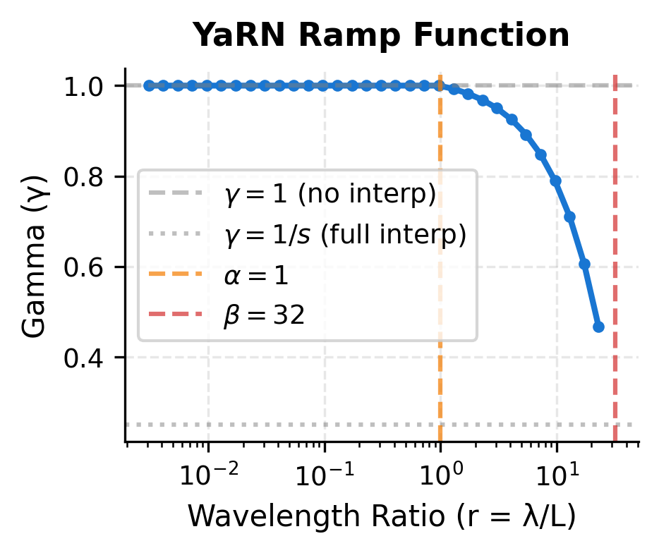
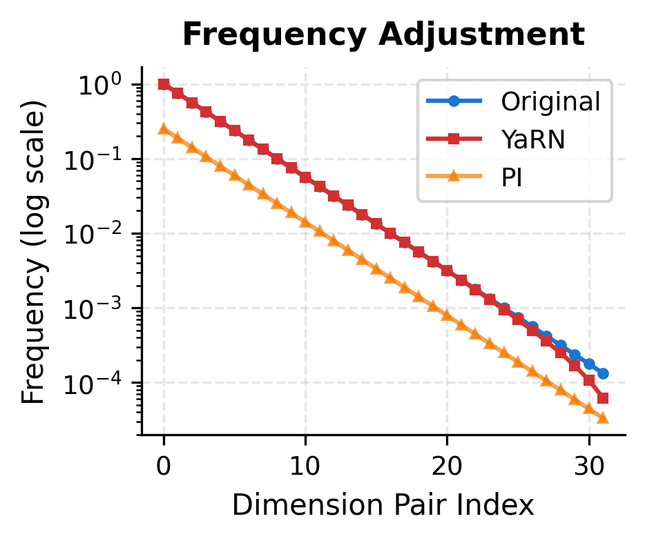
The ramp function creates a piecewise linear transition on the log-wavelength scale. The left panel shows how $\gamma$ drops from 1 to $1/s$ as wavelength increases, with the smooth ramp connecting the two flat regions. The right panel shows the resulting frequency spectrum: YaRN preserves high frequencies at the left side of the dimension range (matching the original), then transitions smoothly to interpolated low frequencies on the right. This dimension-specific adjustment is the key innovation that sets YaRN apart from both PI and NTK-aware scaling.

We've now addressed the frequency problem with the ramp function. But recall that we identified two problems at the start: frequency distortion and entropy shift. Even with perfect frequency adjustments, interpolation changes something fundamental about attention patterns, and the ramp function alone cannot fix it. This is where temperature scaling enters the picture.

To understand why, think about what interpolation does geometrically to the embedding space. When we slow down rotations (by multiplying frequencies by $\gamma < 1$), positions that were previously "far apart" in the rotated embedding space now appear "closer." Consider two tokens at positions 0 and 100. In the original RoPE, dimension pair 0 might rotate these two positions to vectors that are 100 radians apart in angle (after wrapping around the circle many times). With 4x interpolation applied to that pair, the same two positions are rotated to vectors only 25 radians apart. This compression happens across all interpolated dimension pairs simultaneously, and its effect accumulates in the dot product between query and key.

This compression has a direct consequence for attention scores. The dot product between query and key vectors measures their similarity. When positions appear closer together in the rotated space, the dot products become more similar across all pairs of positions. The range of attention scores shrinks: scores that would have spanned, say, $[-3, 3]$ before interpolation might now span only $[-1, 1]$. When this compressed range is passed through softmax, the output distribution becomes flatter.

Recall how softmax works. Given a vector of scores $\mathbf{z}$:

where $z_i$ is the $i$-th attention score and the sum runs over all key positions. When input scores are spread out (high variance), the exponential function amplifies the differences, producing a distribution that peaks strongly at the highest score and falls off quickly. When input scores are compressed (low variance), the exponentials are more similar to each other, producing a flatter distribution. This increased uniformity is precisely what we measure as higher entropy, and it means the model is attending to many positions at once rather than focusing on the most relevant ones.

The solution is conceptually simple: if scores are too compressed, stretch them back out before applying softmax. We do this by multiplying the scores by a factor greater than 1. This is equivalent to reducing the "temperature" in the softmax, which sharpens the output distribution. YaRN frames this as multiplying by $\sqrt{t}$ where $t > 1$. The choice of $\sqrt{t}$ rather than $t$ is deliberate, as we will explain shortly.

The temperature factor $t$ is computed from the extension scale $s$ via a formula derived from empirical fitting across many models and extension factors:

where:

• $t$: the attention temperature scaling factor, always $\geq 1$ for any $s \geq 1$
• $s$: the context extension scale factor (e.g., 4 for 4x extension)
• $\ln(s)$: the natural logarithm of the extension factor
• $0.1$: an empirically determined coefficient that controls how aggressively temperature increases with extension factor
• $1$: the base value ensuring $t = 1$ when $s = 1$, so no correction is applied when there is no extension

Why does this formula use $\ln(s)$ rather than $s$ directly? This reflects an empirical observation about how entropy changes with extension factor. The entropy shift does not grow linearly as we extend further. Going from 4x to 8x extension doubles the context but adds far less than twice the entropy shift that going from 1x to 4x introduced. The logarithm captures this diminishing-returns relationship: doubling the extension factor adds only $\ln(2) \approx 0.693$ to $\ln(s)$, contributing just $0.069$ more to $t$ regardless of where we start. This makes the temperature correction well-calibrated across a wide range of extension factors.

Why $\sqrt{t}$ rather than $t$ directly as the score multiplier? This relates to how variance scales under linear transformation. If we multiply a set of scores by a constant $c$, the variance of the scores is multiplied by $c^2$. To increase variance by a factor of $t$ (undoing the compression from interpolation), we need to multiply scores by $\sqrt{t}$, because $(\sqrt{t})^2 = t$. The choice of $\sqrt{t}$ ensures that the temperature correction acts on the variance of attention scores, not their absolute magnitude, which is the right quantity to adjust for matching entropy.

Temperature scaling moves the entropy closer to the original distribution. While the match is not perfect (which is expected given the fundamental geometric changes to the attention space that interpolation introduces), the correction prevents the excessive entropy increase that would otherwise occur. In practice, the remaining difference is small enough that fine-tuning on long-context data can close the gap entirely, which is why YaRN requires so few fine-tuning steps compared to training from scratch.

Now we can put together the complete YaRN transformation. Given a model trained on context length $L$ that we want to extend by factor $s$, the process involves three coordinated steps. Each step builds on the previous one, and together they constitute the full YaRN algorithm.

Step 1: Compute adjusted frequencies

For each dimension pair $i$ with base frequency $\theta_i$ and wavelength $\lambda_i = 2\pi/\theta_i$, compute the wavelength ratio $r_i = \lambda_i / L$ and the adjusted frequency:

where:

• $\theta'_i$: the adjusted frequency for dimension pair $i$
• $\theta_i$: the original RoPE frequency
• $\gamma(\cdot)$: the ramp function defined in the previous section
• $\lambda_i / L$: the wavelength ratio that determines the amount of interpolation for this dimension

This step is performed once at initialization and the adjusted frequencies are stored. During inference, every query and key vector is rotated using $\theta'_i$ rather than $\theta_i$. The computational cost is identical to standard RoPE; only the frequency values change.

Step 2: Apply RoPE with adjusted frequencies

For query or key vector $\mathbf{x}$ at position $m$, apply the block-diagonal rotation matrix using the adjusted frequencies. Each pair of dimensions $(2i, 2i+1)$ is rotated by angle $\theta'_i \cdot m$:

where:

• $\text{YaRN-RoPE}(\mathbf{x}, m)$: the rotated vector, incorporating YaRN's frequency adjustments
• $R(\theta'_i \cdot m)$: a $2 \times 2$ rotation matrix for angle $\theta'_i \cdot m$, applied to dimension pair $i$
• $\theta'_i \cdot m$: the rotation angle at position $m$, increasing linearly with position at the adjusted rate $\theta'_i$
• The block-diagonal structure means each dimension pair is rotated independently of all others

The rotation matrix $R(\phi)$ for angle $\phi$ is:

This is the standard 2D rotation matrix. Applying it to a pair $(x_{2i}, x_{2i+1})$ gives:

Because rotation is an isometry (it preserves vector lengths), YaRN-RoPE does not change the magnitude of query or key vectors. It only changes their direction, which is all that matters for computing dot products.

Step 3: Apply temperature scaling to attention scores

After computing the raw attention scores from the rotated query and key vectors, apply the temperature correction before softmax:

where:

• $\text{score}(m, n)$: the temperature-scaled attention score between positions $m$ and $n$
• $\mathbf{q}_m$: the YaRN-rotated query vector at position $m$
• $\mathbf{k}_n$: the YaRN-rotated key vector at position $n$
• $d_k$: the dimension of key vectors (the standard $\sqrt{d_k}$ prevents dot products from growing too large)
• $t = 0.1 \ln(s) + 1$: the temperature factor, computed once from the extension scale
• $\sqrt{t}$: the multiplier applied to raw scores, increasing the spread of scores to counteract entropy inflation
• This scaling occurs before the softmax normalization, not after

The implementation confirms that YaRN preserves vector magnitudes (rotation is an isometry) while applying the adjusted frequencies. The extended context (8,192 positions) is 4x larger than the training context (2,048 positions), and the temperature correction of approximately 1.067 will be applied to attention scores before softmax.

Let's trace YaRN's computation for a specific dimension pair to make the mathematics concrete. We'll work through a 4x extension from context length 2,048 to 8,192 with a 64-dimensional model.

Consider dimension pair $i = 10$ (the 11th pair out of 32 total). We'll compute everything step by step.

Step 1: Compute the original frequency.

The base frequency formula gives:

Computing numerically: $10000^{0.3125} = 10^{4 \times 0.3125} = 10^{1.25} \approx 17.78$, so $\theta_{10} \approx 0.0563$.

Step 2: Compute the wavelength.

The wavelength is:

So one complete rotation of dimension pair 10 takes about 112 positions.

Step 3: Compute the wavelength ratio.

With original context $L = 2048$:

Since $r_{10} = 0.054 < \alpha = 1.0$, dimension pair 10 falls in the "no interpolation" region. The model completes about 18 full rotations ($2048 / 111.6 \approx 18.4$) during the training context, so it has learned all possible rotation states.

Step 4: Apply the ramp function.

Since $r_{10} < \alpha$, we have $\gamma(r_{10}) = 1$. The adjusted frequency is:

Dimension pair 10 is unchanged: it rotates at its original speed.

Now let's examine dimension pair $i = 28$ (near the low-frequency end).

Step 1: Compute the original frequency.

Step 2: Compute the wavelength.

One full rotation of dimension pair 28 takes over 35,000 positions.

Step 3: Compute the wavelength ratio.

Since $1.0 < r_{28} = 17.25 < 32.0 = \beta$, dimension pair 28 falls in the ramp (transition) region.

Step 4: Apply the ramp function.

The linear weight is:

The interpolation factor is:

The adjusted frequency is:

Dimension pair 28 is slowed down to about 61% of its original speed. With the extended context of 8,192 positions, a token at position 8,192 would produce a rotation angle of $\theta'_{28} \times 8192 \approx 0.884$ radians, which corresponds to about 14% of a full rotation. The model has learned rotation states up to about $\theta_{28} \times 2048 = 0.1778 \times 2048 = 0.364$ radians in the original training, so 0.884 radians is outside the training distribution. The gamma correction reduces this to $\theta'_{28} \times 8192 \approx 0.884$ radians... wait, let's check with the corrected frequency: $0.0001079 \times 8192 \approx 0.884$ radians. Pair 28 still extrapolates somewhat (since we applied only partial interpolation), which is intentional. Full interpolation would be too conservative; partial interpolation strikes a balance between accessing new context and staying close to the training distribution.

Step 5: Temperature correction.

For $s = 4$:

The attention score multiplier is $\sqrt{1.139} \approx 1.067$. Every pre-softmax attention score is multiplied by this factor before the softmax is applied.

This worked example shows the key principle: YaRN applies a per-dimension decision based on physical intuition (how much of the rotation cycle has been trained), rather than a global formula that treats all dimensions identically.

Let's visualize how YaRN affects the attention patterns compared to other methods. A good visualization helps build the intuition for why YaRN's two-part correction produces qualitatively better attention distributions.

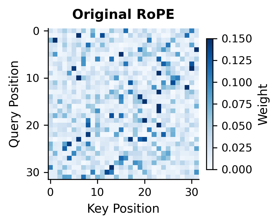
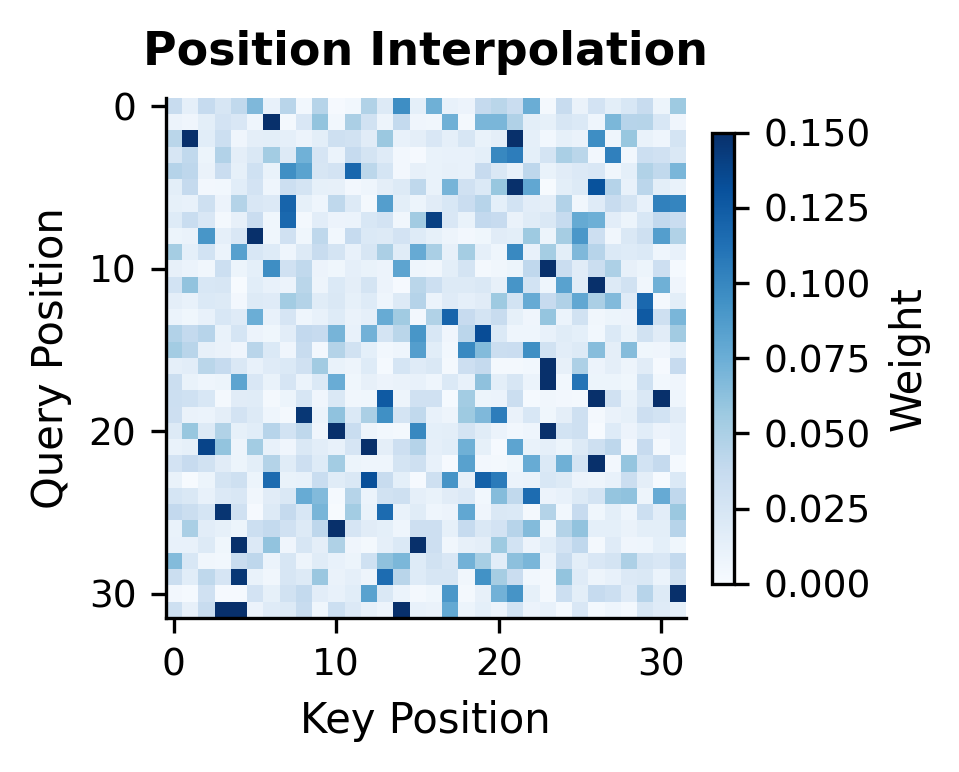
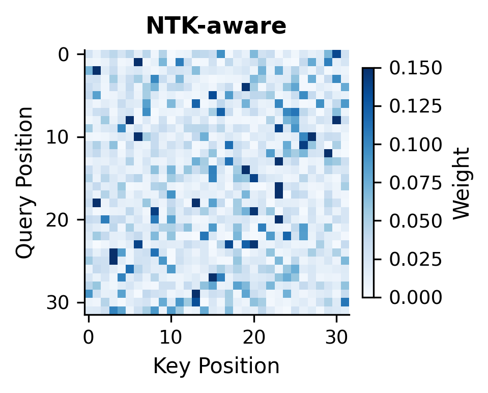
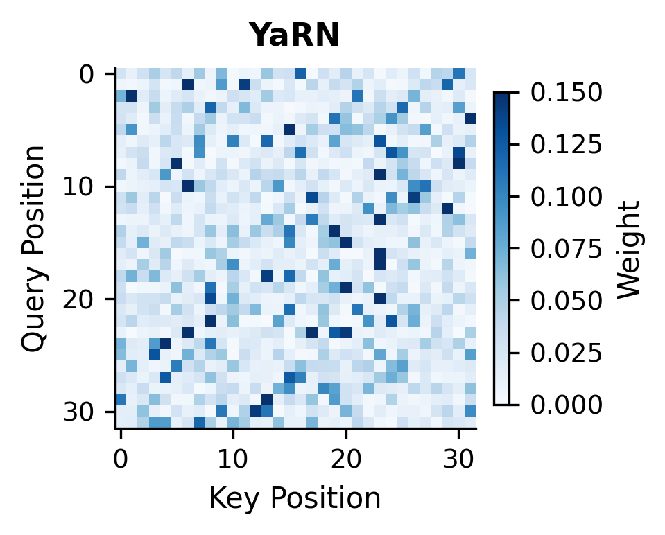
The attention heatmaps reveal the qualitative differences between methods at a 16x extension factor, where differences are most pronounced. Position Interpolation produces the most diffuse patterns: the uniform compression of all frequencies flattens the attention distribution across all key positions. NTK-aware scaling improves upon this by preserving high-frequency discrimination, resulting in slightly more structured patterns. YaRN, combining selective interpolation with temperature correction, produces patterns that most closely resemble the original RoPE baseline, with sharper peaks and clearer structure in the weight distribution. This visual comparison explains why YaRN requires less fine-tuning to recover model quality: it starts from a better position, and the model's existing weights need fewer updates to adapt.

An important practical consideration is whether YaRN requires fine-tuning on long-context data. The answer depends on the extension factor, and understanding the relationship between extension factor and fine-tuning need helps practitioners plan deployments.

For modest extensions (2x to 4x), YaRN can often be applied without any fine-tuning at all. The frequency adjustments and temperature scaling are designed to minimize the distribution shift, and for small extension factors, the shift is small enough that the model's existing weights remain effective. Many practitioners have successfully used YaRN zero-shot at 2x extension for models like LLaMA-2 and Mistral, obtaining usable quality without any additional training.

For larger extensions (8x to 32x), brief fine-tuning significantly improves quality. The YaRN paper recommends 200 to 400 training steps on long-context data, which is dramatically less than training from scratch (which requires billions of tokens) or even than Position Interpolation typically needs at the same extension factor. The key is that YaRN's adjustments start the model in a more compatible state: the model's learned attention patterns are closer to what they need to be, so the fine-tuning process has less work to do.

For extreme extensions (64x and beyond), longer fine-tuning becomes necessary, though still much shorter than pre-training from scratch. At these extreme factors, even YaRN's carefully designed corrections cannot prevent some distributional drift, and the model needs to develop new strategies for handling positions that are truly far outside its original training distribution.

The key advantage of YaRN over naive approaches is the efficiency of this fine-tuning. Because the method preserves the essential structure of the position encoding while making targeted adjustments, the model needs to learn only minor adaptations rather than fundamentally new position representations. Think of it as teaching a fluent speaker of one dialect to understand another: the core language knowledge transfers; only the specific patterns need updating. Compare this to Position Interpolation at large extension factors, where the model may need to essentially relearn position-sensitive behavior from scratch.

Now that we understand YaRN in depth, let's compare it with other RoPE extension methods. Each method makes different trade-offs, and understanding those trade-offs helps you choose the right approach for a given situation.

Position Interpolation is the simplest approach: divide all position indices by the extension factor $s$. Its main strength is conceptual simplicity and ease of implementation. Its weakness is the uniform compression of all frequencies, which loses high-frequency position discrimination. For small extension factors and after adequate fine-tuning, PI performs well. For larger factors or in low-data regimes, the loss of high-frequency information becomes problematic.

NTK-aware scaling improves upon PI by working at the level of the base frequency rather than the position indices. By increasing the base from 10,000 to a larger value, NTK-aware scaling adjusts the entire frequency spectrum in a non-uniform way: high-frequency components are preserved better, while low-frequency components receive more aggressive scaling. This makes NTK-aware scaling more reliable than PI at moderate extension factors. The limitation is that it still applies a single global transformation to all dimension pairs: there is no mechanism for giving individual pairs exactly the treatment they need.

Dynamic NTK scaling extends NTK-aware scaling by making the base adjustment position-dependent: at the beginning of a sequence, the base is unchanged, and it gradually increases as the sequence grows longer. This allows the model to start with standard RoPE behavior and transition smoothly to extended behavior within a single sequence. The downside is complexity and some reported training instability at very large extension factors.

YaRN takes a more targeted approach by analyzing each dimension pair individually and applying the appropriate amount of interpolation based on that pair's specific wavelength relative to the training context. The ramp function enables dimension-specific control that the global transformations used by the other methods cannot achieve. The temperature correction adds a second layer of targeted adjustment, addressing the entropy problem that none of the other methods account for.

The main advantages of YaRN are:

1. Selective preservation: High-frequency dimensions that don't need interpolation are left unchanged, maintaining fine-grained position discrimination. This is the key advantage over PI.

2. Entropy control: Temperature scaling prevents the attention distribution from becoming too diffuse. This is the key advantage over all other methods, which do not address entropy at all.

3. Efficient adaptation: The targeted adjustments require less fine-tuning to adapt to than more disruptive methods. Models using YaRN reach quality targets with fewer gradient steps.

4. Predictable behavior: The ramp function provides interpretable control over which dimensions are interpolated and by how much, making it easier to understand and diagnose.

The "Mean Entropy" column shows how diffuse the attention distribution is. Lower values indicate sharper, more focused attention: the model is attending strongly to a few positions rather than spreading attention evenly. The "Rel. Pos. Error" measures whether the same relative distance produces the same attention score at different absolute positions: a value near zero indicates that the position encoding is truly relative (consistent across the sequence), while larger values indicate positional inconsistency.

The comparison shows that YaRN achieves entropy closest to the original RoPE baseline while maintaining good relative position consistency. The combination of targeted interpolation (keeping high-frequency pairs at their original frequencies) and temperature scaling (pushing entropy back toward the original distribution) produces the best overall match with the original behavior that the model was trained with.

Despite its effectiveness, YaRN has limitations worth understanding carefully before deploying it in production systems. Being aware of these limitations helps you apply YaRN appropriately and avoid pitfalls.

Hyperparameter sensitivity: The $\alpha$ and $\beta$ parameters control the ramp function's transition region, and their optimal values can vary between model architectures. The defaults of $\alpha = 1$ and $\beta = 32$ were validated on LLaMA-2 and Mistral models with standard RoPE bases of 10,000. Models with different RoPE bases (some newer models use bases of 500,000 or higher), different dimension sizes, or different training context lengths may require retuning these parameters. The good news is that the parameters have clear interpretations: $\alpha$ sets the wavelength-ratio threshold below which no interpolation is applied, and $\beta$ sets the threshold above which full interpolation is applied. You can reason about their values by inspecting the wavelength distribution for your specific model.

Temperature approximation: The formula $t = 0.1 \ln(s) + 1$ is empirically derived rather than theoretically optimal. It was fit to match entropy behavior across several models and extension factors, but it is not guaranteed to perfectly compensate for entropy shifts in all scenarios. For models with very different attention score distributions (due to different training regimes or architectural choices), the coefficient 0.1 may not be ideal. In practice, the sensitivity to this coefficient is low: varying it between 0.07 and 0.15 produces similar quality, so the default is usually adequate.

Integration complexity: Unlike Position Interpolation (which only modifies position indices) or NTK-aware scaling (which only modifies the base frequency), YaRN requires two separate modifications: the ramp function for frequencies and the temperature scaling for attention scores. Both must be implemented correctly and at the right points in the computation. In particular, the temperature scaling must occur at the pre-softmax stage of attention, not before or after. When integrating YaRN into existing model code, it is easy to accidentally apply the frequency adjustment but forget the temperature correction (or vice versa), resulting in degraded performance.

Interaction with other optimizations: When combined with techniques like FlashAttention or grouped-query attention, care must be taken to apply the temperature scaling at the correct point in the computation. FlashAttention fuses the attention computation into a single kernel and may require the temperature factor to be folded into the $\sqrt{d_k}$ denominator as $\sqrt{d_k / t}$ rather than applied as a separate multiplication. Grouped-query attention (GQA) shares key and value heads across multiple query heads, so the temperature should be applied per attention score, not per head. These are implementation details rather than fundamental limitations, but they require attention when deploying YaRN in optimized inference frameworks.

Long-document retrieval challenges: Even with YaRN, models can struggle with certain long-context tasks. Retrieval of specific facts from very long documents (the "needle in a haystack" problem) often degrades at extreme context lengths even with YaRN applied, because the model may develop implicit biases about where important information appears in a sequence. Fine-tuning on diverse long-context data, including examples where the relevant information appears at many different positions, is essential for achieving reliable long-context retrieval.

These limitations are manageable in practice. YaRN has been successfully integrated into many open-source models and inference frameworks, including the Mistral-7B extended context variants and numerous LLaMA-based community models. The community has developed reference implementations that handle the integration details correctly, making it straightforward to apply YaRN to a new model using existing code as a template.

When implementing YaRN for a new model, several parameters control its behavior. Understanding what each controls makes it easier to configure YaRN correctly and tune it when needed.

• scale: The context extension factor (e.g., 4.0 for extending from 2048 to 8192 tokens). This is the most important parameter and must be set to the ratio of the desired context length to the original training context length. Larger values enable longer contexts but may require more fine-tuning to reach full quality.

• alpha: The lower wavelength threshold (default: 1.0). Dimension pairs with wavelength-to-context ratio below this value receive no interpolation. Setting $\alpha = 1$ means any pair whose wavelength fits within the training context is left untouched. Decreasing $\alpha$ below 1 would apply interpolation to some pairs that complete full rotations during training, which is generally unnecessary. Increasing $\alpha$ would apply less interpolation overall, potentially causing extrapolation for pairs with wavelengths slightly above the context length.

• beta: The upper wavelength threshold (default: 32.0). Dimension pairs with wavelength-to-context ratio above this value receive full interpolation. Increasing $\beta$ delays full interpolation to pairs with longer wavelengths, applying partial interpolation over a wider range. Decreasing $\beta$ would apply full interpolation earlier, which could be appropriate for models where even moderately slow-moving pairs have not generalized well to unseen rotation states.

• base: The RoPE frequency base (default: 10000). This should match the base used in the original model's RoPE implementation exactly. Using the wrong base shifts all wavelength computations and causes the ramp function to apply interpolation to the wrong dimension pairs. Many recent models (released in 2024 onward) use higher bases like 500,000, which significantly shifts the wavelength distribution and may require re-examining the $\alpha$ and $\beta$ thresholds.

• original_context: The context length the model was originally trained on (e.g., 2048 or 4096). This determines the wavelength ratios used in the ramp function. Getting this wrong would cause YaRN to apply the wrong amount of interpolation to each dimension pair.

For most applications, the default values of $\alpha = 1$ and $\beta = 32$ work well. The primary parameter to adjust is scale, which should be set to the desired extension factor. If the model uses a non-standard RoPE base, ensure base matches the original configuration. And if you observe poor long-context quality after fine-tuning, consider whether the $\alpha$ and $\beta$ thresholds are appropriate for your model's specific wavelength distribution.

YaRN provides a principled and practically effective approach to extending context length in RoPE-based language models. By combining selective frequency interpolation via the ramp function with attention temperature scaling, it addresses the two distinct problems that simpler methods leave unsolved: frequency distortion and entropy shift.

The key insight driving YaRN is that different dimension pairs in RoPE have fundamentally different needs. High-frequency pairs (short wavelengths) have learned the full rotation cycle during training and can handle extended positions without modification. Low-frequency pairs (long wavelengths) have only seen a small arc of their rotation cycle and need interpolation to avoid extrapolation. The ramp function encodes this insight directly, applying a dimension-specific decision based on each pair's wavelength ratio $r_i = \lambda_i / L$.

The temperature correction addresses a separate problem: even with perfect frequency adjustments, interpolation compresses the geometry of the rotated embedding space. This makes all keys look more similar to every query and flattening the attention distribution. The formula $t = 0.1 \ln(s) + 1$ provides a calibrated correction that grows logarithmically with the extension factor. The logarithmic form matches the empirical observation that entropy shift saturates rather than growing linearly.

Key takeaways:

• Wavelength-based interpolation: YaRN uses a ramp function to apply no interpolation to high-frequency dimension pairs, full interpolation to low-frequency pairs, and a smooth transition in between. This preserves fine-grained position information where it matters.

• Attention temperature correction: Context extension increases attention entropy. YaRN compensates with a temperature scaling factor $\sqrt{t}$ where $t = 0.1 \ln(s) + 1$, applied to pre-softmax scores.

• Efficient fine-tuning: The targeted adjustments minimize distribution shift, enabling effective context extension with as few as 200 to 400 fine-tuning steps for moderate extension factors.

• Complementary to other methods: YaRN can be seen as a refinement that combines insights from Position Interpolation (full interpolation for long wavelengths) and NTK-aware scaling (preservation of short wavelengths), while adding the novel temperature correction that addresses entropy.

• Practical deployment: YaRN has been integrated into many open-source models and inference frameworks. This shows its practical viability for real-world context extension at scales from 4x to 32x.

The next chapter explores attention sinks, a phenomenon where transformer models allocate disproportionate attention to initial tokens regardless of their semantic relevance, and how this affects long-context processing.

Ready to test your understanding? Take this quick quiz to reinforce what you've learned about YaRN and its approach to extending context length in RoPE-based models.