

Explore how large language models learn new tasks from prompt demonstrations without weight updates. Covers example selection, scaling behavior, and theoretical explanations.

This article is part of the free-to-read Language AI Handbook
Choose your expertise level to adjust how many terms are explained. Beginners see more tooltips, experts see fewer to maintain reading flow. Hover over underlined terms for instant definitions.
In-Context Learning
When GPT-3 was released in 2020, researchers observed something unexpected: the model could perform new tasks simply by being shown a few examples in the prompt, without any gradient updates or fine-tuning. This capability, called in-context learning (ICL), represented a fundamental shift in how we think about adapting language models to new tasks. Rather than collecting labeled datasets and training specialized models, you could now demonstrate a task through examples and let the model infer what to do.
This chapter explores in-context learning in depth. We'll examine why it works, how it compares to traditional fine-tuning, what makes some examples more effective than others, how ICL capabilities scale with model size, and the theoretical frameworks researchers have developed to explain this surprising phenomenon.
What Is In-Context Learning?
In-context learning refers to a language model's ability to learn new tasks from examples provided in the input prompt, without updating any model parameters. The model "learns" the task pattern by conditioning on the demonstrations and applies that pattern to new inputs.
In-context learning (ICL) is the ability of a pretrained language model to perform a task by conditioning on a few input-output examples (demonstrations) in the prompt, without any gradient-based training or weight updates. The model infers the task from the examples and generalizes to new inputs.
Consider a translation task. Instead of fine-tuning a model on thousands of parallel sentences, you can provide a few examples directly in the prompt:
English: The weather is beautiful today.
French: Le temps est magnifique aujourd'hui.

English: I would like a cup of coffee.
French: Je voudrais une tasse de café.

English: Where is the nearest train station?
French:
The model completes this with "Où est la gare la plus proche?" having inferred the translation pattern from just two examples. No training occurred. The model's weights remain unchanged. Yet it performs the task correctly.
This behavior was surprising because traditional machine learning assumes you need gradient updates to learn. The model must see many examples, compute a loss, and adjust its parameters. ICL breaks this assumption: learning happens within a single forward pass through the network.
The Three Regimes of Prompting
The GPT-3 paper formalized three prompting regimes based on how many examples are provided:
Each regime has distinct characteristics:
- Zero-shot: The model relies entirely on its pretrained knowledge and the task description. Works best for common tasks the model encountered during pretraining.
- One-shot: A single example clarifies the expected format and task. Often sufficient for simple classification or formatting tasks.
- Few-shot: Multiple examples help the model distinguish between classes, understand edge cases, and calibrate its confidence. Typically 4-32 examples, limited by context length.
The number of examples you can provide is constrained by the model's context window. With a 2,048 token limit (GPT-3) or 8,192+ tokens (later models), you must balance demonstration count against prompt length.
ICL vs Fine-Tuning
Traditional task adaptation requires fine-tuning: updating a pretrained model's weights on task-specific labeled data. In-context learning offers an alternative that trades training for inference. Understanding when to use each approach requires examining their fundamental differences.
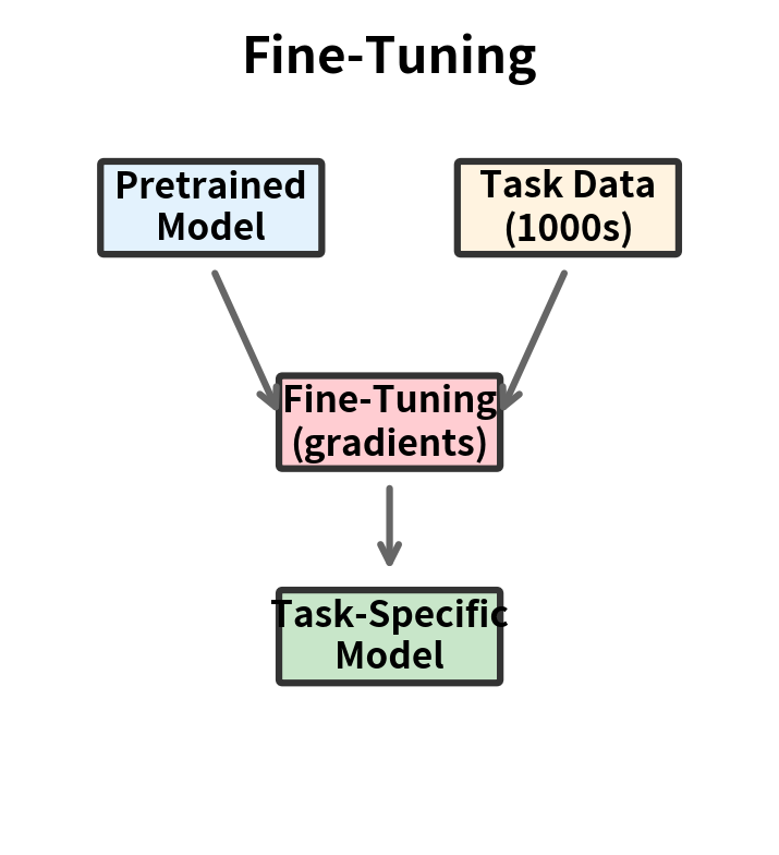
The Fine-Tuning Paradigm
Fine-tuning involves several steps:
- Collect labeled examples for your task (typically thousands)
- Initialize from a pretrained model
- Train on your data with gradient descent
- Deploy the specialized model
The result is a dedicated model for your task. Its weights have been permanently modified to excel at that specific application. Fine-tuning produces strong performance but requires:
- Labeled training data
- Compute for training
- Expertise to avoid overfitting
- Separate model storage per task
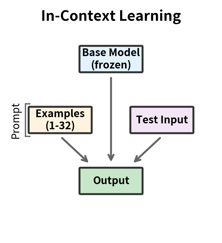
The ICL Paradigm
In-context learning follows a different path:
- Prepare a small number of demonstrations (typically 1-32)
- Format them into a prompt
- Pass the prompt to the base model at inference time
The base model remains unchanged. The same model serves all tasks, with demonstrations specifying what to do. ICL requires no training but consumes inference compute for longer prompts.
Comparing Performance
How do these approaches compare in practice? The answer depends on several factors:
| Aspect | Fine-Tuning | In-Context Learning |
|---|---|---|
| Data required | 100s-1000s of examples | 1-32 examples |
| Training time | Hours to days | None |
| Inference cost | Standard | Higher (longer prompts) |
| Task switching | Load new model | Change prompt |
| Peak performance | Generally higher | Competitive for many tasks |
| Model updates | New base model requires retraining | Automatic improvement |
Fine-tuning typically achieves higher accuracy when sufficient training data is available. The model has many gradient steps to learn task-specific patterns. ICL is limited to what can be demonstrated in a prompt and what the model learned during pretraining.
However, ICL excels in scenarios where fine-tuning is impractical:
- Rapid prototyping: Test ideas without training infrastructure
- Low-resource tasks: Limited labeled data available
- Dynamic tasks: Task definition changes frequently
- Multi-task deployment: Single model serves many tasks
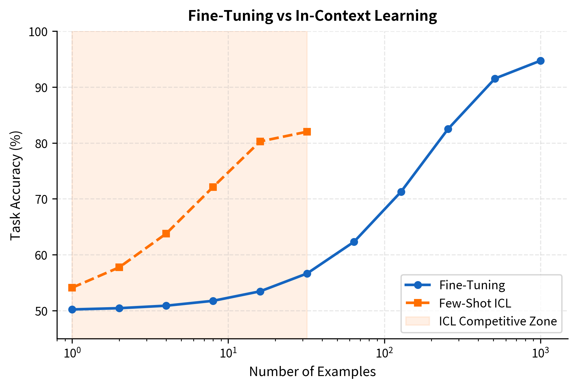
The crossover point varies by task. For simple classification, ICL often matches fine-tuning with just a few examples. For complex reasoning or structured prediction, fine-tuning's advantage is more pronounced.
When Representations Converge
Recent research shows that ICL and fine-tuning produce similar internal representations despite their different mechanisms. When you examine the hidden states of a model performing a task via ICL versus a fine-tuned version of that model, the representations are often highly correlated.
This suggests that both approaches activate similar "circuits" in the network. Fine-tuning strengthens these circuits through weight updates. ICL activates them through attention over demonstrations. The end result, in terms of what the model computes, is quite similar.
Example Selection Strategies
Not all demonstrations are equally effective. Research has shown that the choice of examples can swing performance by 20-30 percentage points. Understanding what makes examples effective has become a critical skill in prompt engineering.
Factors That Influence Example Quality
Several properties affect how useful an example is as a demonstration:
- Relevance: Examples similar to the test input help more than dissimilar ones
- Diversity: Examples should cover the range of possible inputs and outputs
- Clarity: Unambiguous examples with clear input-output relationships work best
- Correctness: Erroneous labels can mislead the model
- Ordering: Examples at the end of the prompt have stronger influence
Let's examine each factor and how to optimize for it.
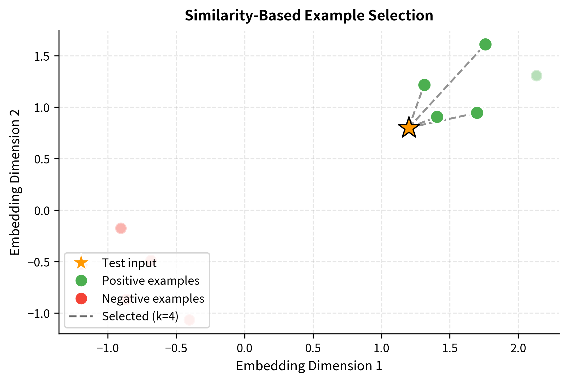
Semantic Similarity Selection
One of the most effective strategies is selecting examples that are semantically similar to the test input. The intuition is that nearby examples in embedding space share relevant features that help the model generalize.
Similarity is typically measured using cosine similarity between embedding vectors:
where:
- and : embedding vectors for two text inputs
- : the dot product of the two vectors
- and : the Euclidean norms (lengths) of each vector
Cosine similarity ranges from -1 (opposite directions) to 1 (identical directions), with 0 indicating orthogonal (unrelated) vectors. For text embeddings, higher similarity indicates semantically related content.
The selection algorithm identifies examples that are semantically closest to the test input. In this case, the mock embedder produces consistent but randomized vectors, so the selected examples demonstrate the general approach. In practice, using a real sentence embedding model like sentence-transformers would select examples with genuinely similar meaning and vocabulary.
Similarity-based selection consistently outperforms random selection. The most similar examples contain vocabulary, style, and semantic features that help the model understand what kind of input it's processing.
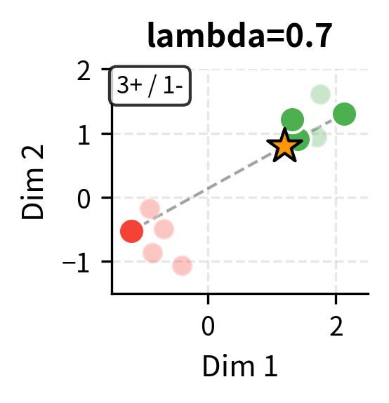
Diversity Through Coverage
While similarity helps, relying solely on it can create blind spots. If all selected examples are too similar, the model may not learn to handle edge cases or the full range of outputs.
A balanced approach selects examples that are both relevant and diverse:
Unlike pure similarity-based selection, MMR actively penalizes redundancy. The diversity weight of 0.3 means the algorithm balances 70% relevance with 30% diversity. This typically results in better class coverage, as selecting multiple very similar examples provides diminishing returns.
The maximal marginal relevance (MMR) algorithm iteratively selects examples that are relevant to the query but dissimilar to already-selected examples. At each step, MMR scores each candidate using:
where:
- : a candidate demonstration being evaluated
- : the query (test input) we want to find examples for
- : the set of already-selected demonstrations
- : similarity between candidate and query (relevance term)
- : maximum similarity between candidate and any already-selected example (redundancy term)
- : diversity weight balancing relevance versus diversity (typically 0.3-0.5)
The first term rewards candidates similar to the query. The second term penalizes candidates similar to already-selected examples. By subtracting the redundancy term, MMR prevents selecting demonstrations that are too similar to each other, ensuring coverage of diverse aspects of the task.
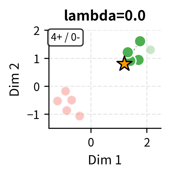

Class-Balanced Selection
For classification tasks, ensuring balanced representation across classes is critical. If your demonstrations are skewed toward one class, the model may be biased toward predicting that class.
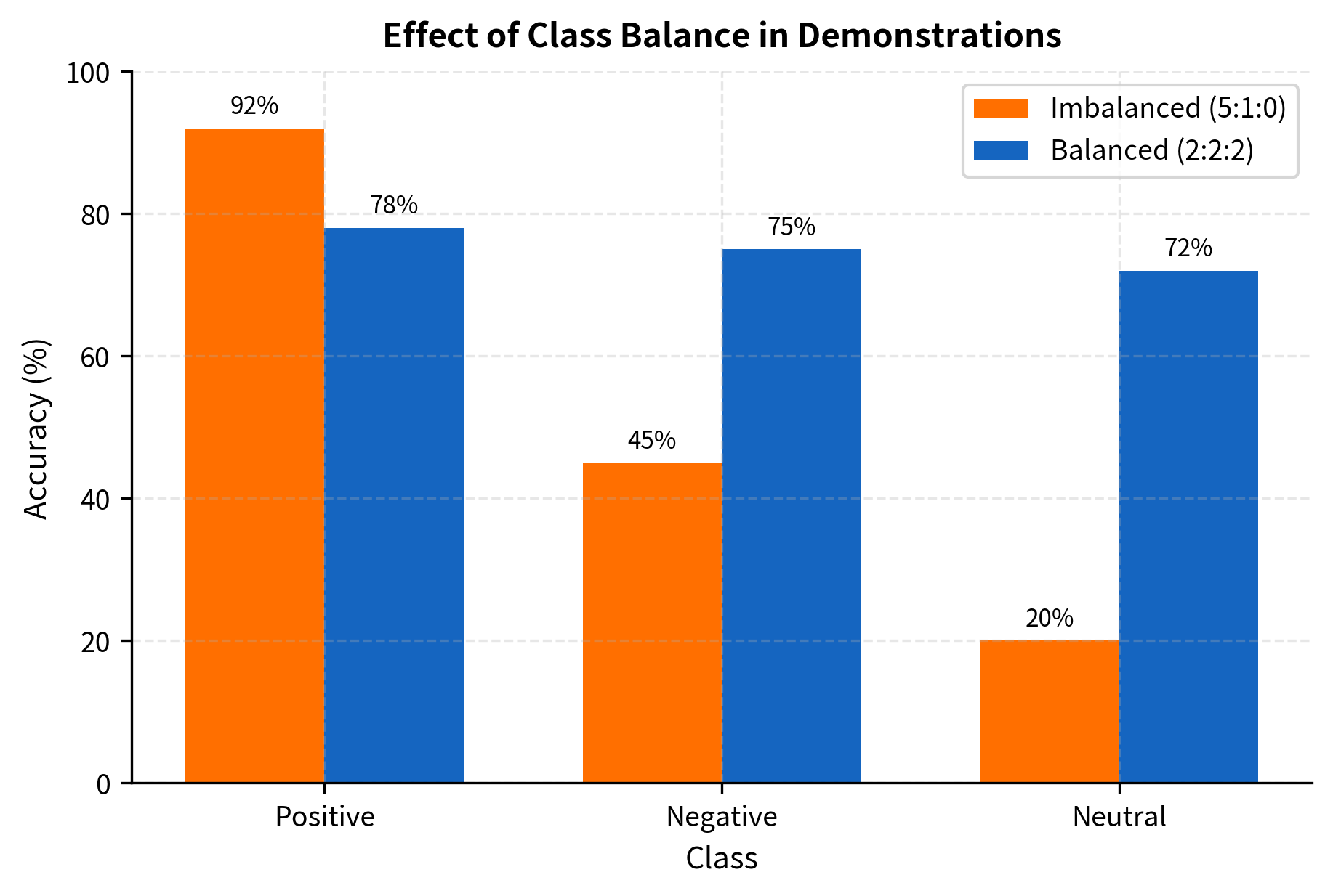
The effect of class imbalance can be dramatic. In extreme cases, providing examples from only one class causes the model to predict that class for all inputs, regardless of the actual content.
Ordering and Recency Effects
The order of examples in the prompt matters more than you might expect. Examples closer to the test input (at the end of the prompt) tend to have stronger influence on the prediction. This "recency effect" emerges from the attention mechanism, where nearby tokens naturally receive more attention.
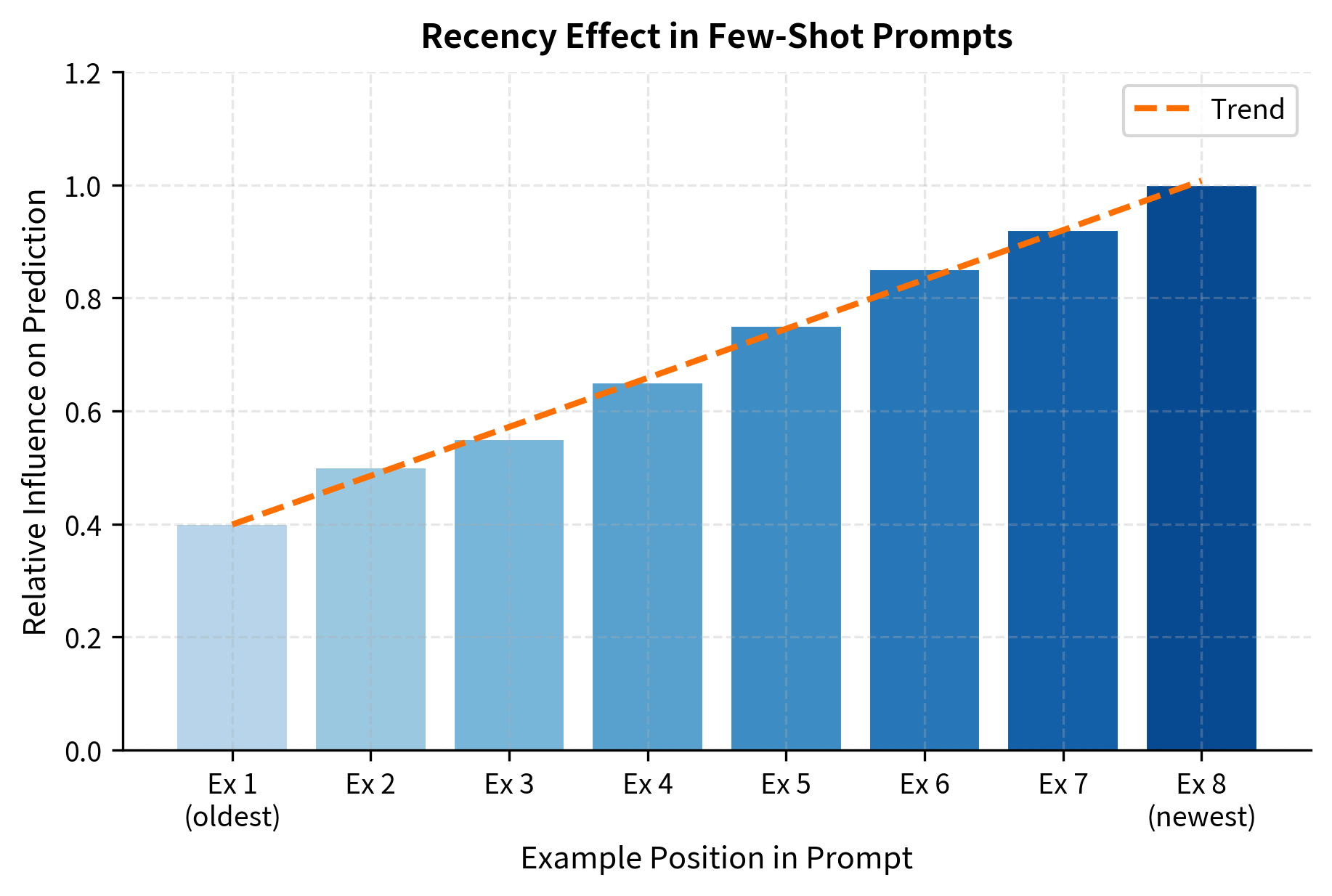
Practical implications of the recency effect:
- Place the most representative examples at the end of the prompt
- When class-balancing, ensure the final examples aren't all from one class
- For tasks with a default or majority class, counterbalance by ending with minority examples
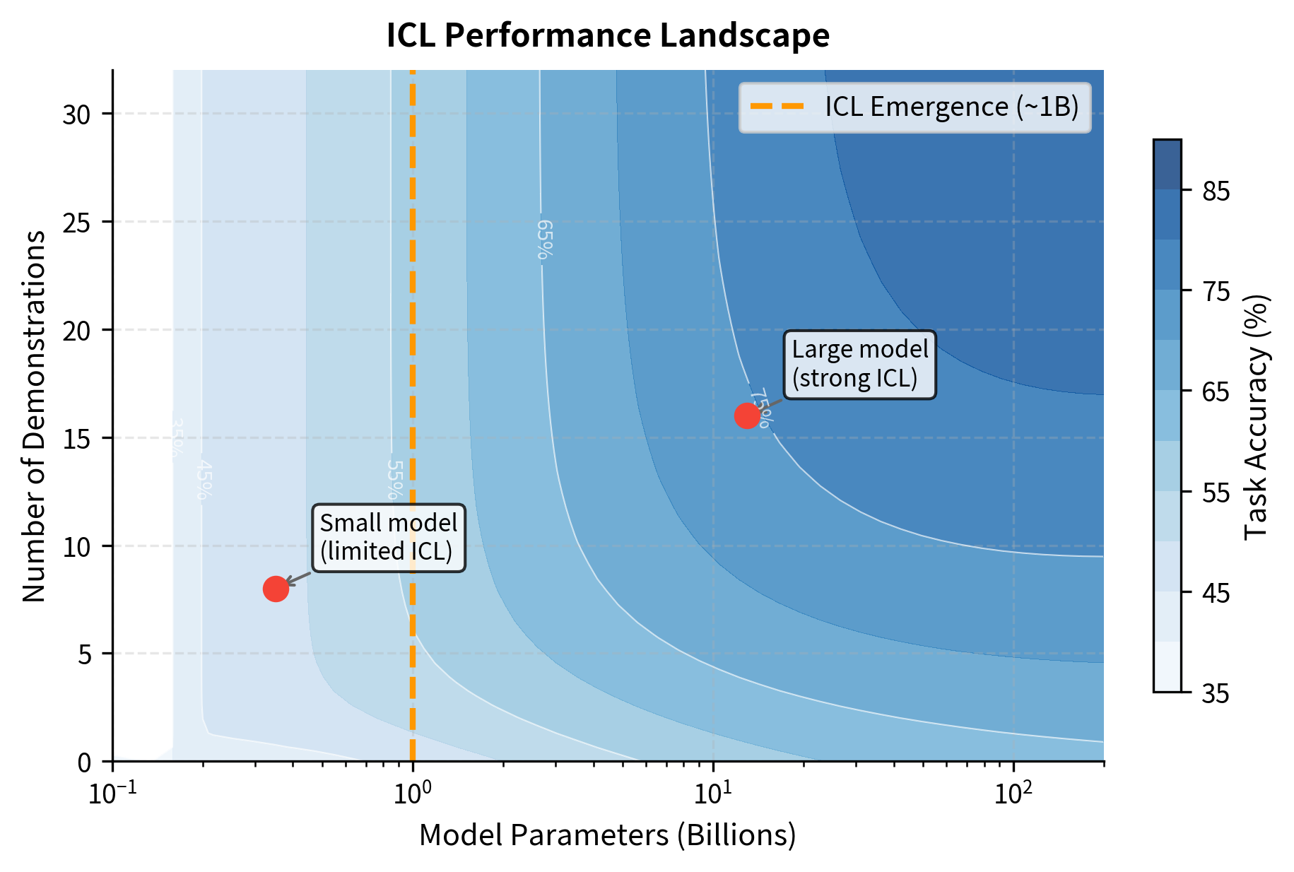
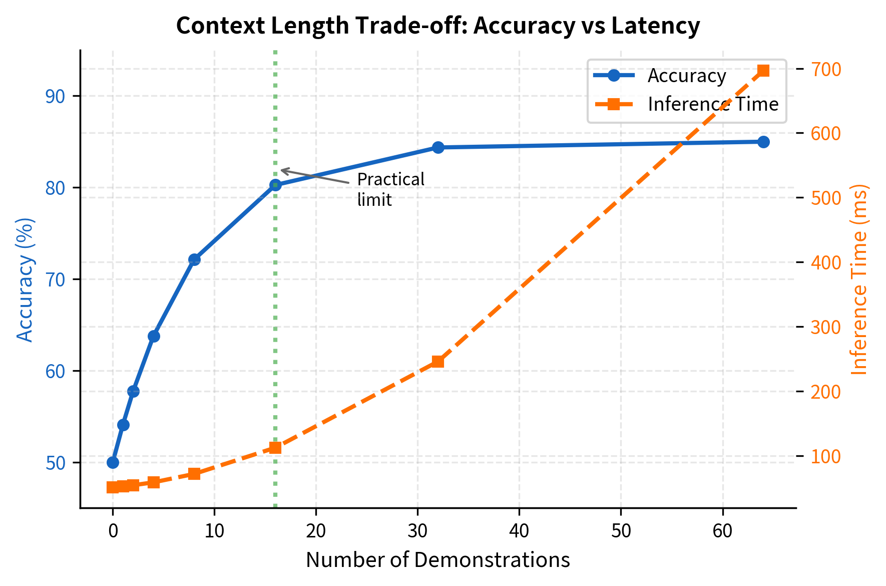
ICL Scaling Behavior
One of the most interesting aspects of in-context learning is how it scales. Both the number of examples and the model size affect performance, but the relationship is not simply additive.
More Examples Help (Up to a Point)
Adding more demonstrations generally improves performance, but with diminishing returns. The first few examples provide the largest gains, while additional examples contribute less.
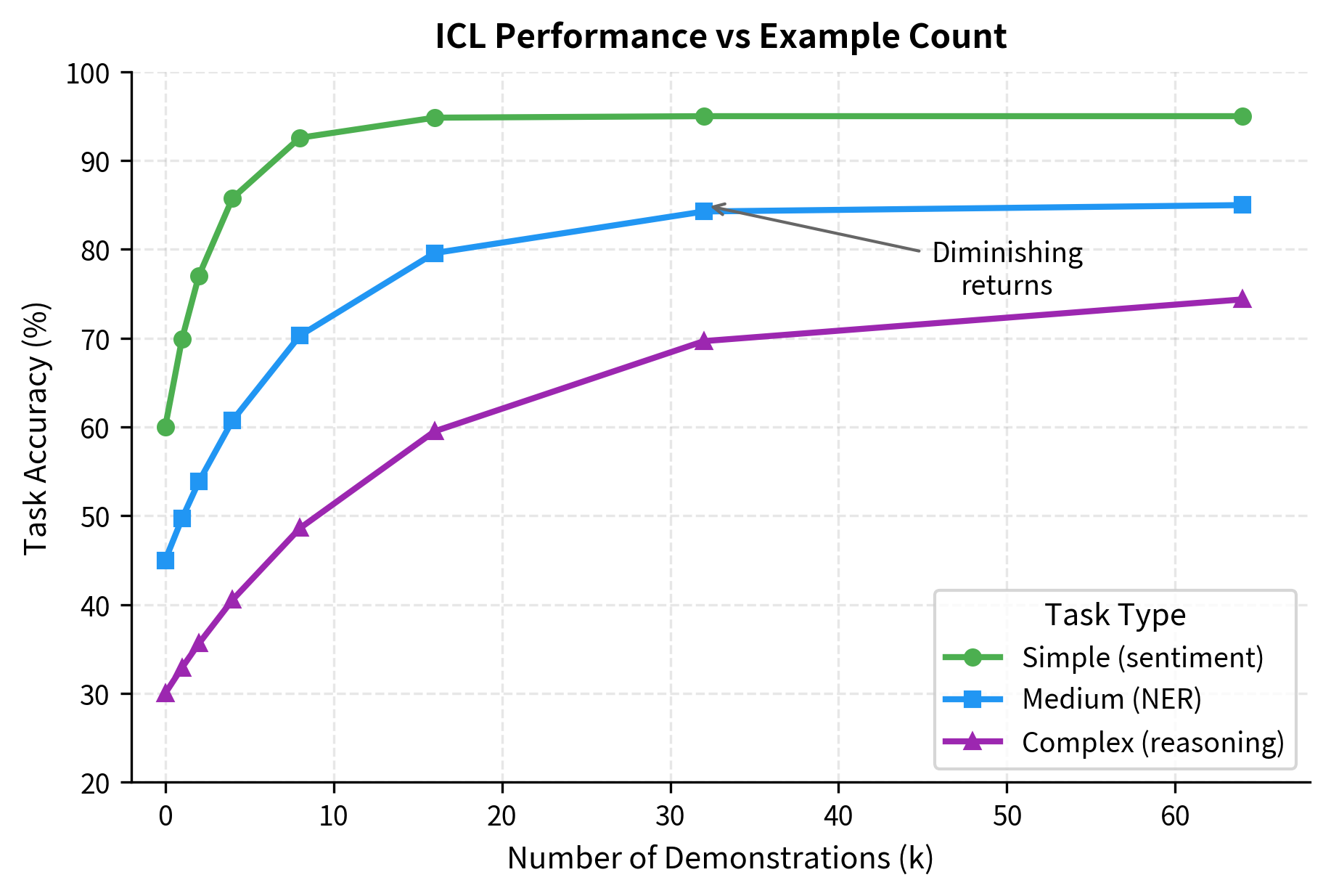
The optimal number of examples depends on:
- Task complexity: Simple tasks need fewer examples
- Model capacity: Larger models extract more from each example
- Example quality: High-quality examples provide more information per demonstration
- Context budget: Longer examples leave less room for more demonstrations
Model Size Enables ICL
The most dramatic scaling effect is the relationship between model size and ICL capability. Small models show minimal benefit from demonstrations. As models grow larger, they become increasingly able to leverage in-context examples.
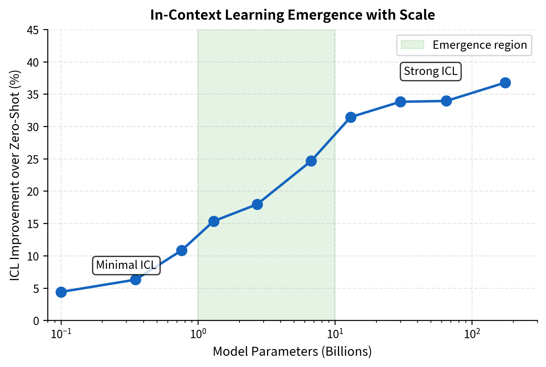
This emergence pattern has important implications. It suggests that in-context learning is not simply scaling up pattern matching but represents a qualitatively different capability that activates at sufficient scale. Models below a certain threshold don't just do ICL poorly; they essentially don't do it at all.
The Interplay of Scale and Examples
Model size and example count interact in interesting ways. Larger models:
- Extract more information from each example
- Continue improving with more examples for longer
- Generalize better from diverse demonstrations
- Are more robust to example ordering and selection
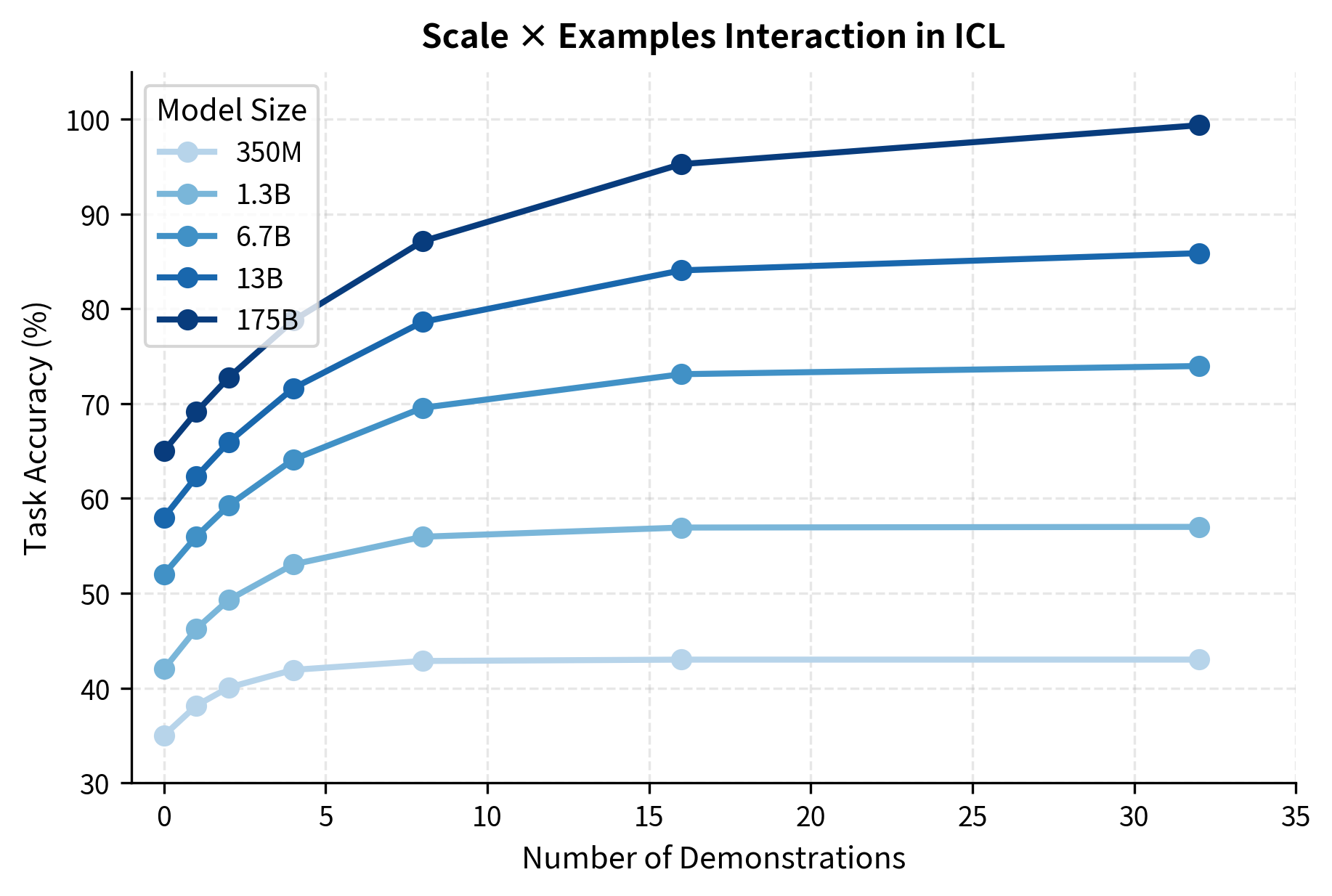
The practical takeaway: if you're working with a smaller model, investing heavily in example selection and count may not pay off. But with large models, careful prompt engineering with well-chosen examples can yield substantial gains.
Theoretical Understanding of ICL
How can a model "learn" without updating its weights? This question strikes at the heart of what makes in-context learning so puzzling. In traditional machine learning, learning requires gradient descent: the model sees examples, computes errors, and adjusts its parameters to reduce those errors over many iterations. ICL appears to violate this fundamental requirement. A frozen model, with weights fixed at their pretrained values, somehow adapts its behavior based on demonstrations it has never seen before.
Understanding this phenomenon requires thinking carefully about what "learning" actually means in the context of a forward pass through a neural network. Three complementary hypotheses have emerged from theoretical research, each illuminating a different aspect of how ICL works. We'll explore each in turn, building from intuition to mathematical formalization.
Hypothesis 1: Task Location
The first hypothesis reframes the question: perhaps ICL doesn't involve learning at all in the traditional sense. Instead, demonstrations might serve as a kind of address that locates pre-existing knowledge.
Consider what happens during pretraining. The model processes billions of tokens from diverse sources: Wikipedia articles, books, code repositories, forums, and countless other text formats. Within this ocean of data, the model implicitly encounters many task formulations:
- Question-answer pairs embedded in FAQ pages and forums
- Translation examples in multilingual documents
- Sentiment expressions in reviews and social media
- Factual statements in encyclopedic content
- Code with natural language comments and docstrings
The key insight is that pretraining doesn't just teach the model to predict the next token. It teaches the model to recognize patterns and activate appropriate processing strategies. When you provide few-shot demonstrations, you're not teaching the model something new. Instead, you're helping it identify which of its existing capabilities to apply.
Think of it like a library with millions of books but no catalog. The model has all the knowledge, but it needs help finding the right book. Demonstrations serve as search queries that locate the relevant "section" of the model's capabilities.
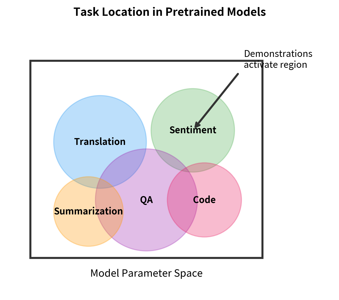
Several lines of evidence support the task location hypothesis:
- ICL works best for familiar tasks: Performance is highest on tasks similar to those encountered during pretraining, suggesting the model is retrieving existing capabilities rather than learning new ones.
- Novel operations fail: Tasks requiring genuinely new logical operations that couldn't have been learned from text data tend to fail at ICL, even with many demonstrations.
- Task descriptions can substitute for examples: Sometimes a natural language description of the task works as well as demonstrations, which makes sense if the goal is location rather than learning.
The task location view is intuitive, but it doesn't fully explain the mechanics. How does the model actually use demonstrations to activate the right capabilities? This leads us to our second hypothesis.
Hypothesis 2: Implicit Gradient Descent
While the task location hypothesis tells us what ICL accomplishes, the implicit gradient descent hypothesis explains how the transformer architecture actually implements this process. The key insight is that the attention mechanism, when viewed mathematically, performs operations that closely resemble gradient descent.
To understand this connection, we need to examine what happens during a single attention layer. When the model processes a prompt containing demonstrations followed by a test input, the attention mechanism allows information to flow from the demonstrations to the test input.
Consider the query input (the test case we want the model to complete). Before attention, it has some initial representation . The attention mechanism then updates this representation by aggregating information from the demonstrations:
where:
- : the updated representation of the query input after attention
- : the initial representation of the query input before this attention layer
- : the attention weight assigned to demonstration , computed via softmax over query-key dot products
- : the value vector derived from demonstration , encoding information about that example
- : the total number of demonstrations in the prompt
This formula has the same structure as a gradient descent update. In standard gradient descent, we update parameters by:
where represents the current parameters, is the learning rate, and is the gradient of the loss. The analogy becomes clear when we make the following correspondences:
| Gradient Descent | Attention Mechanism |
|---|---|
| Current parameters | Initial representation |
| Learning rate | Attention weights |
| Gradient | Value vectors |
| Updated parameters | Updated representation |
The attention weights act as adaptive, example-specific learning rates. They automatically assign more weight to demonstrations that are more relevant (those with higher query-key similarity). This is actually more sophisticated than standard gradient descent, where the learning rate is typically fixed.
Research has substantiated this connection with increasingly strong results:
- Constructive proofs: Researchers have shown that transformers can be explicitly constructed to implement gradient descent algorithms.
- Linear attention equivalence: For linear attention layers (without the softmax nonlinearity), the forward pass is mathematically equivalent to one step of gradient descent on a regression problem.
- Multi-step optimization: With 96 layers like GPT-3, the model can implement many sequential "optimization steps," allowing for sophisticated adaptation to the demonstrations.
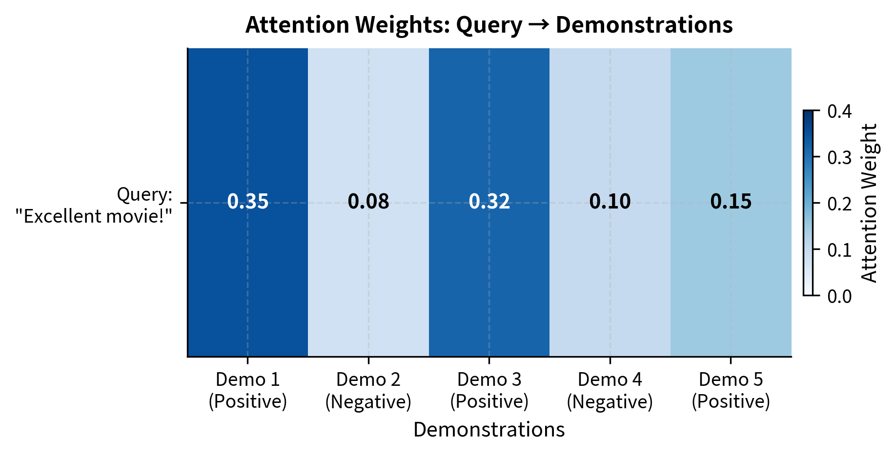
The attention weights reveal how the model allocates "learning" across demonstrations. Demo 1 and Demo 3 (both Positive) receive higher weights because their embeddings are more similar to the query. Demo 2 (Negative) receives lower weight due to its dissimilar embedding. The updated representation shifts toward the weighted average of demonstrations, with the shift magnitude indicating how much the query representation changed.
This toy example captures the essence of the implicit gradient descent hypothesis: demonstrations don't just provide information, they actively reshape the query representation through the attention mechanism. Similar examples contribute more to this reshaping, just as training examples with larger gradients contribute more to parameter updates in standard learning.
Hypothesis 3: Bayesian Inference
The first two hypotheses focus on mechanism: what capabilities exist (task location) and how attention implements adaptation (implicit gradient descent). Our third hypothesis takes a probabilistic perspective, asking: how does the model's uncertainty about the task change as it sees more demonstrations?
Imagine you're trying to guess what game someone is playing by watching them take actions. Each action provides evidence about which game it might be. Early on, many games are plausible. As you observe more actions, your beliefs concentrate on the correct game. This is exactly what Bayesian inference formalizes.
Applied to ICL, the model starts with a prior distribution over possible tasks, learned during pretraining. This prior reflects how often different task types appeared in the training data. When you provide demonstrations, each one updates this distribution according to Bayes' rule:
where:
- : the -th demonstration, consisting of an input and its corresponding output
- : the prior probability of each task type, reflecting how often the model encountered similar patterns during pretraining
- : the likelihood of observing these specific demonstrations if the task is as hypothesized (demonstrations consistent with the task have high likelihood)
- : the posterior probability of each task after observing all demonstrations
- : indicates proportionality (the left side equals the right side divided by a normalizing constant)
Let's trace through this formula step by step to build intuition:
-
The prior encodes pretraining knowledge. If the model saw many sentiment classification examples during pretraining, sentiment analysis has a higher prior probability than, say, a specialized domain-specific task.
-
The likelihood evaluates consistency. For each possible task interpretation, how likely is it that we would observe these specific demonstrations? If the demonstrations show text mapped to "Positive" and "Negative" labels, the likelihood is high under "sentiment classification" and low under "translation."
-
The posterior concentrates probability. Multiplying prior and likelihood (and normalizing) yields a posterior that combines our initial beliefs with the evidence from demonstrations. As more demonstrations are added, the posterior becomes sharper, concentrating on the task interpretation that best explains all the evidence.
This Bayesian view explains several empirical observations about ICL:
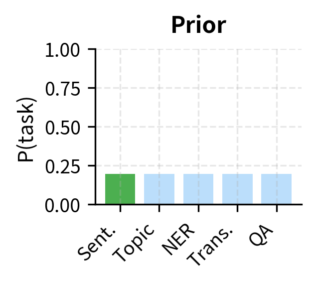
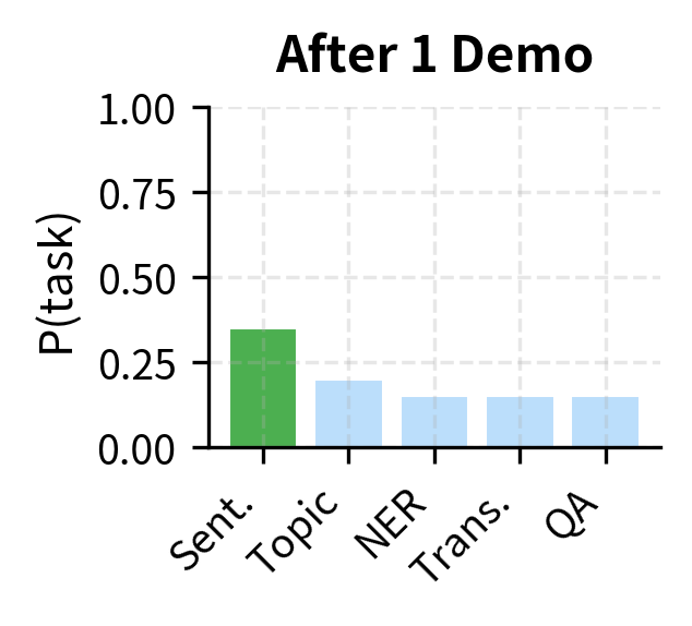
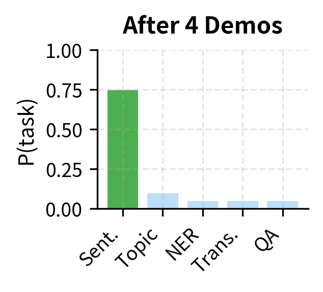
The visualization illustrates how the posterior evolves. Initially, probability is spread uniformly across task interpretations. After one demonstration showing an input mapped to "Positive," the posterior shifts toward sentiment classification. After four demonstrations consistently showing sentiment labels, the model has high confidence in the task identity.
Evidence supporting the Bayesian view comes from several empirical observations:
- Inconsistent demonstrations hurt performance. If you mix correct and incorrect labels, the likelihood term is reduced for all task interpretations, leading to a diffuse posterior and poor predictions.
- Ambiguous prompts yield uncertain outputs. When demonstrations could plausibly come from multiple tasks, the model's predictions are less confident, exactly as a diffuse posterior would predict.
- More examples help even when redundant. Providing 16 similar examples rather than 4 can improve performance, because each example sharpens the posterior even if it doesn't add new information.
Synthesizing the Theories
These three hypotheses are not competing explanations but rather complementary perspectives on the same phenomenon. Each answers a different question:
| Hypothesis | Question Answered |
|---|---|
| Task Location | What capabilities can ICL access? |
| Implicit Gradient Descent | How does attention implement adaptation? |
| Bayesian Inference | How does uncertainty reduce with evidence? |
A unified view might work like this: During pretraining, the model develops specialized circuits for different tasks (task location). When demonstrations are provided, the attention mechanism adapts the query representation toward these demonstrations (implicit gradient descent), which has the effect of concentrating probability on task interpretations consistent with the evidence (Bayesian inference).
Recent theoretical work has made this unified view more concrete. Researchers have shown that transformers, through their architecture, learn to implement meta-learning algorithms during pretraining. When presented with demonstrations at inference time, they execute these algorithms to infer the task and generate appropriate predictions. The specific algorithm implemented may vary by layer, attention head, and task type, with different components of the network contributing different aspects of the adaptation process.
Improving ICL Performance
Researchers have developed numerous techniques to enhance in-context learning beyond simple few-shot prompting.
Chain-of-Thought Prompting
For reasoning tasks, showing intermediate steps significantly improves performance. Instead of just input-output pairs, demonstrations include the reasoning process:
Chain-of-thought (CoT) prompting guides the model to show its work. The reasoning trace helps the model:
- Break complex problems into steps
- Catch and correct errors mid-reasoning
- Align intermediate computations with the final answer
CoT is particularly effective for arithmetic, logical reasoning, and multi-step problems where the direct answer is hard to compute in a single step.
Self-Consistency
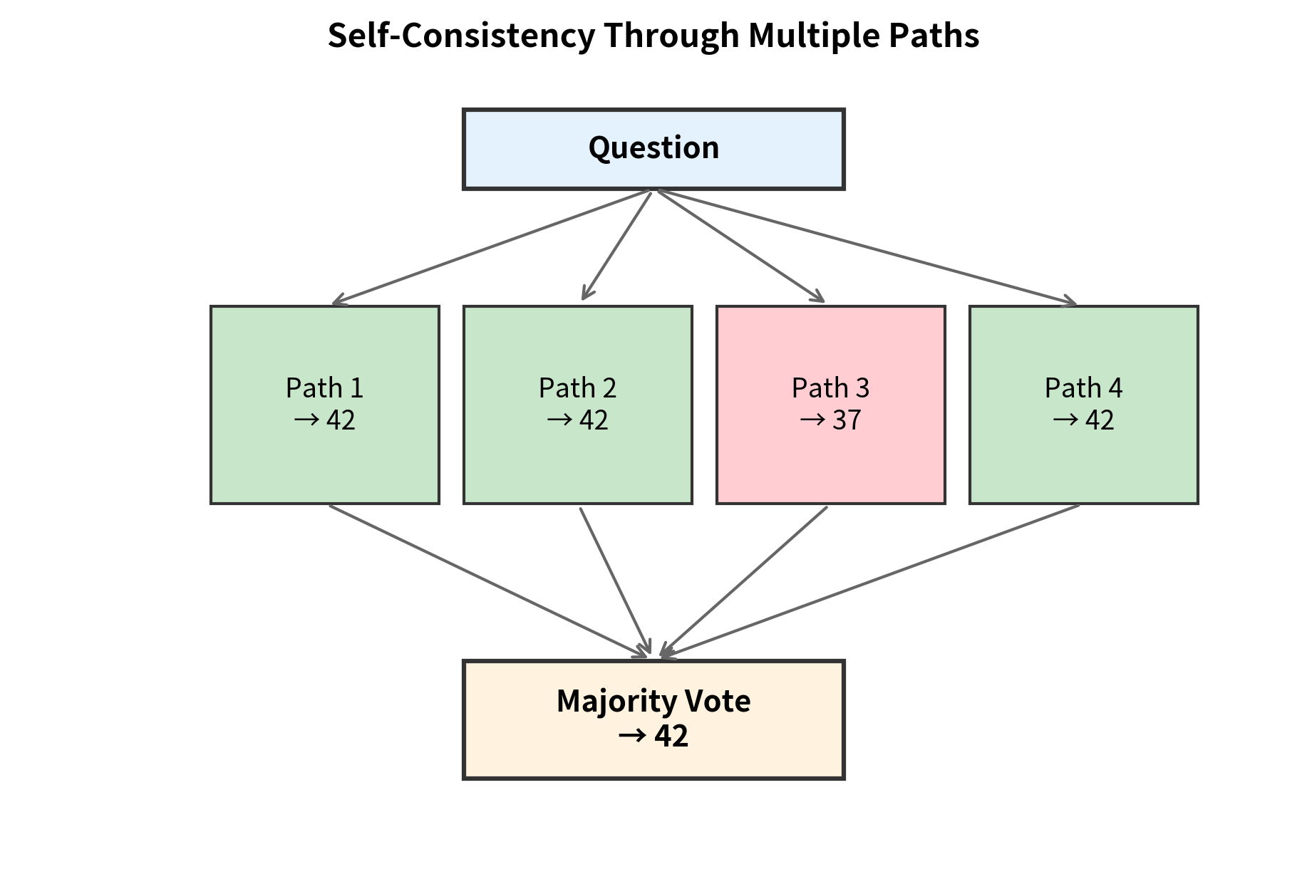
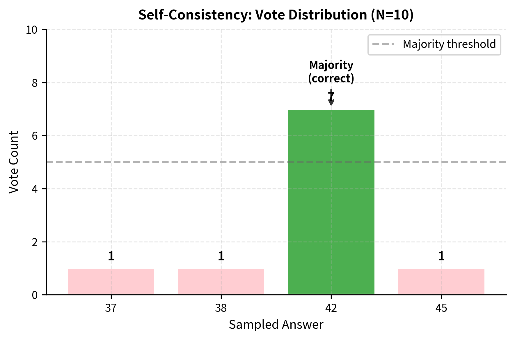
Rather than generating a single answer, self-consistency samples multiple reasoning paths and aggregates them through majority voting. The procedure works as follows:
- Generate different chain-of-thought responses using temperature to introduce diversity
- Extract the final answer from each response
- Return the most common answer (majority vote)
Formally, the self-consistency prediction is:
where:
- : the final predicted answer
- : the number of sampled reasoning paths
- : the answer extracted from the -th reasoning path
- : an indicator function that equals 1 if answer matches , and 0 otherwise
- : selects the answer that maximizes the vote count
This approach leverages the intuition that correct reasoning paths, while potentially different in details, converge on the same answer. Incorrect paths are more likely to diverge, producing different wrong answers that split the vote. With enough samples, the correct answer accumulates more votes than any single incorrect answer.
Calibration and Confidence
ICL predictions can be overconfident or poorly calibrated. Several techniques address this:
- Probability calibration: Adjust output probabilities using held-out validation data
- Verbalizing uncertainty: Ask the model to express confidence in its answer
- Null prompts: Compare predictions with and without demonstrations to detect when the model is guessing
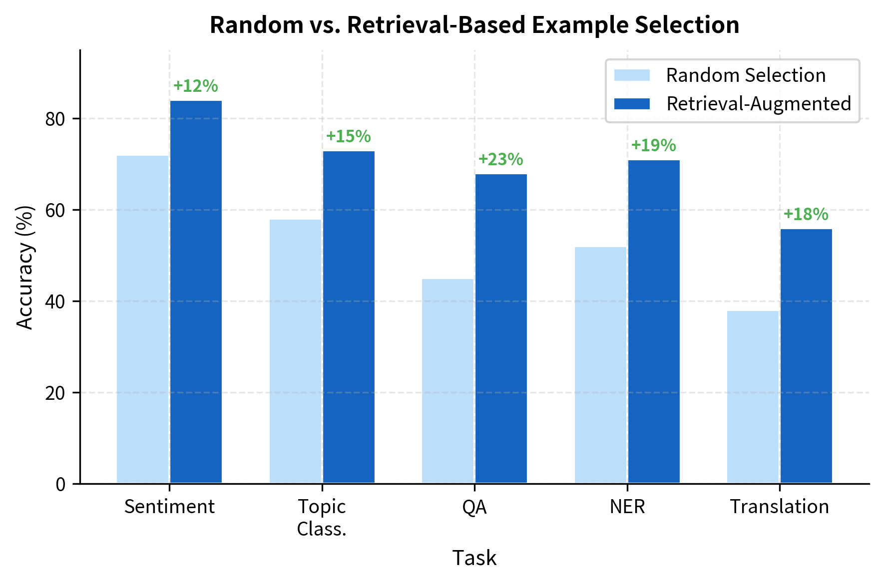
Retrieval-Augmented ICL
Instead of using a fixed set of demonstrations, retrieval-augmented approaches dynamically select examples for each test input:
- Embed the test input
- Retrieve similar examples from a large pool
- Use retrieved examples as demonstrations
This combines the benefits of similarity-based selection with the scalability of large example pools. The model effectively has access to thousands of potential demonstrations, selecting the most relevant ones at inference time.
Limitations of In-Context Learning
ICL has fundamental limitations that practitioners should understand.
Context Length Constraints
The number of demonstrations is bounded by the model's context window. With 4,096 tokens, you might fit 10-20 examples depending on their length. This hard limit constrains what ICL can learn from a single prompt.
Long-context models (32K, 100K+ tokens) partially address this, but attention over very long contexts introduces its own challenges: slower inference, potential loss of focus, and quadratic memory scaling.
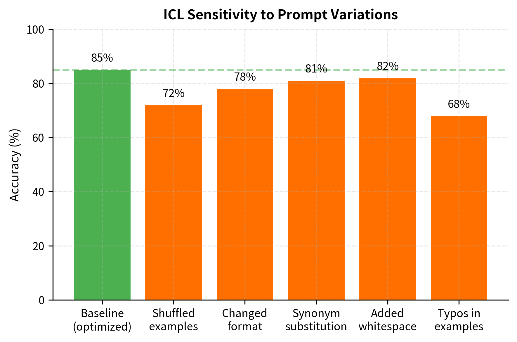
Sensitivity to Irrelevant Details
ICL is sensitive to aspects of the prompt that shouldn't matter:
- Formatting: Changing delimiters or spacing affects predictions
- Order: Shuffling examples changes accuracy
- Wording: Synonymous task descriptions yield different results
- Few irrelevant tokens: Adding noise degrades performance
This brittleness makes reliable deployment challenging. A prompt optimized on development data may fail unexpectedly on edge cases.
No Permanent Learning
ICL provides only temporary task adaptation. Each new inference requires providing demonstrations again. The model doesn't retain any information between queries. For frequently repeated tasks, this overhead can be significant compared to a fine-tuned model that encodes the task permanently.
Limited Task Complexity
Some tasks are too complex to demonstrate in a few examples. Tasks requiring:
- Extensive domain knowledge
- Multi-step procedures with many steps
- Precise output formats (structured data, code)
- Consistency across a long document
often exceed what ICL can reliably achieve. Fine-tuning or more sophisticated architectures may be necessary.
Summary
In-context learning has changed how we adapt language models to new tasks. Rather than training specialized models, we demonstrate tasks through examples and let the model infer what to do.
Key takeaways:
-
ICL is weight-free learning: The model performs new tasks by conditioning on demonstrations, without any gradient updates. This enables rapid task switching and prototyping.
-
Example selection matters enormously: Choosing relevant, diverse, and balanced examples can swing performance by 20+ percentage points. Strategies like similarity-based selection and MMR help optimize demonstration quality.
-
ICL scales with model size: Small models show minimal ICL capability. The ability to learn from demonstrations emerges around 1-10 billion parameters and continues improving with scale.
-
Multiple theories explain ICL: Task location (activating existing capabilities), implicit gradient descent (attention as optimization), and Bayesian inference (updating task posteriors) offer complementary perspectives on why ICL works.
-
Techniques can enhance ICL: Chain-of-thought prompting, self-consistency, and retrieval augmentation extend what ICL can achieve, particularly for reasoning tasks.
-
Limitations persist: Context length constraints, prompt sensitivity, lack of permanent learning, and task complexity bounds constrain what ICL can reliably accomplish.
In-context learning has changed how NLP is practiced. Tasks that once required careful dataset curation and model training can now be prototyped in minutes with a few well-chosen examples. Understanding both its capabilities and limitations is important for effective application.
Key Parameters
When designing in-context learning prompts, several parameters significantly affect performance:
-
k (number of demonstrations): The count of input-output examples included in the prompt. Start with 4-8 examples for most tasks. Simple classification may need only 2-4, while complex reasoning benefits from 16-32. More examples generally help but with diminishing returns, and you're constrained by context length.
-
diversity_weight (): In MMR-based example selection, this parameter balances relevance (similarity to test input) versus diversity (dissimilarity to already-selected examples). Values of 0.3-0.5 typically work well. Higher values (0.5-0.7) prioritize coverage across the input space; lower values (0.1-0.3) prioritize relevance to the specific test case.
-
temperature: When using self-consistency or sampling multiple outputs, temperature controls randomness. Use 0.0 for deterministic outputs, 0.7-1.0 for diverse reasoning paths in self-consistency. Higher temperatures increase diversity but may reduce coherence.
-
N (self-consistency samples): The number of reasoning paths to sample before majority voting. Common values are 5-40. More samples improve reliability but increase cost linearly. For critical applications, 20-40 samples provide robust estimates; for rapid prototyping, 5-10 may suffice.
-
example ordering: Place the most representative or highest-quality examples at the end of the prompt (closest to the test input) due to recency effects. For classification, ensure the final 2-3 examples aren't all from the same class.
-
prompt format: The delimiter style, spacing, and structure of demonstrations. Consistent formatting across examples helps the model recognize the pattern. Common formats include "Input: X / Output: Y" or "Q: X / A: Y". Match the format to what the model likely saw during pretraining.
Quiz
Ready to test your understanding? Take this quick quiz to reinforce what you've learned about in-context learning.

Comments