Whole Word Masking: Eliminating Information Leakage in BERT Pre-training

When BERT tokenizes "undeniably" into ["un", "##deni", "##ably"] and then masks only "##ably", something goes wrong. The model sees "un" and "##deni" in the clear, giving it strong hints about the masked portion. The prediction task becomes almost trivial: what word starts with "undeni-" and ends with a common suffix? This partial visibility undermines the learning objective.

Whole Word Masking (WWM) fixes this by treating subword tokens as parts of atomic units. If any subword of a word is selected for masking, all subwords of that word are masked together. The model must now predict the entire word from surrounding context alone, without peeking at sibling subwords. This seemingly simple change produces meaningful improvements in downstream task performance.

In this chapter, we'll examine why subword masking creates problems, how whole word masking works algorithmically, and how to implement it for different tokenizers. We'll also compare WWM against random subword masking to see the empirical differences.

Modern language models use subword tokenization to handle vocabulary efficiently. Algorithms like WordPiece, BPE, and SentencePiece break words into smaller units based on frequency or likelihood. Common words remain intact while rare words decompose into recognizable pieces.

This decomposition creates an asymmetry in the masking process. When we randomly select 15% of tokens for masking, we're selecting subword tokens, not words. A multi-token word might have some subwords masked while others remain visible. The visible subwords leak information about the masked ones.

Consider how BERT processes the sentence "The transformation was remarkable." Using WordPiece tokenization:

If random masking selects only "##ation", the input becomes:

The model sees "transform" immediately adjacent to the mask. How many English words start with "transform-"? Only a handful: transformation, transformed, transforming, transformer. The prediction task collapses from choosing among 30,000 vocabulary items to distinguishing between 3-4 suffixes.

This is problematic for several reasons:

• Weak learning signal: The model learns to pattern-match subword combinations rather than understand context deeply. It doesn't need to reason about meaning, just morphology.

• Uneven difficulty: Single-token words face the full prediction challenge while multi-token words get easy hints. The model develops uneven representations.

• Distributional mismatch: During fine-tuning, the model sees complete words. Pre-training on partial words creates a distribution shift.

To understand exactly how much information leaks when sibling subwords are visible, we need a way to measure uncertainty. How hard is the prediction task? Information theory gives us a precise tool: entropy.

The intuition behind entropy

Imagine you're playing a guessing game. If someone picks a number between 1 and 1,000, you have high uncertainty. If they pick between 1 and 2, you have low uncertainty. Entropy quantifies this: it measures how many "bits" of information you need to identify the answer. More possible answers means higher entropy; fewer means lower.

For language model predictions, entropy captures how "spread out" the model's probability distribution is. When the model is confident about one token, entropy is low. When it's unsure between many tokens, entropy is high. A good training signal comes from high entropy: the model must work hard to make the right prediction.

The entropy formula

Given a masked position, the model outputs a probability distribution over all possible tokens. The conditional entropy of this prediction is:

where:

• $H(x_{\text{mask}} | x_{\text{context}})$: the conditional entropy of the masked token given visible context, measured in bits (if using $\log_2$) or nats (if using natural log)
• $x_{\text{mask}}$: the masked token the model must predict
• $x_{\text{context}}$: the visible tokens surrounding the masked position
• $V$: the vocabulary of all possible tokens
• $P(v | x_{\text{context}})$: the probability of token $v$ being the correct prediction given the context

The formula works by taking each possible token, weighting its log-probability by the probability itself, and summing. High probability on one token means $P \cdot \log P$ is large and negative for that token but near zero for others, yielding low total entropy. Uniform probability across many tokens means many moderate contributions, yielding high entropy.

Entropy bounds tell us about task difficulty

Two extreme cases illuminate the formula's behavior:

1. Maximum entropy: When all $|V|$ tokens are equally likely, each has probability $1/|V|$, and entropy reaches $\log |V|$. For a vocabulary of 30,000 tokens, that's about 15 bits: a genuinely challenging prediction.

2. Minimum entropy: When one token has probability 1.0 and all others have probability 0, entropy equals 0. The prediction is trivial.

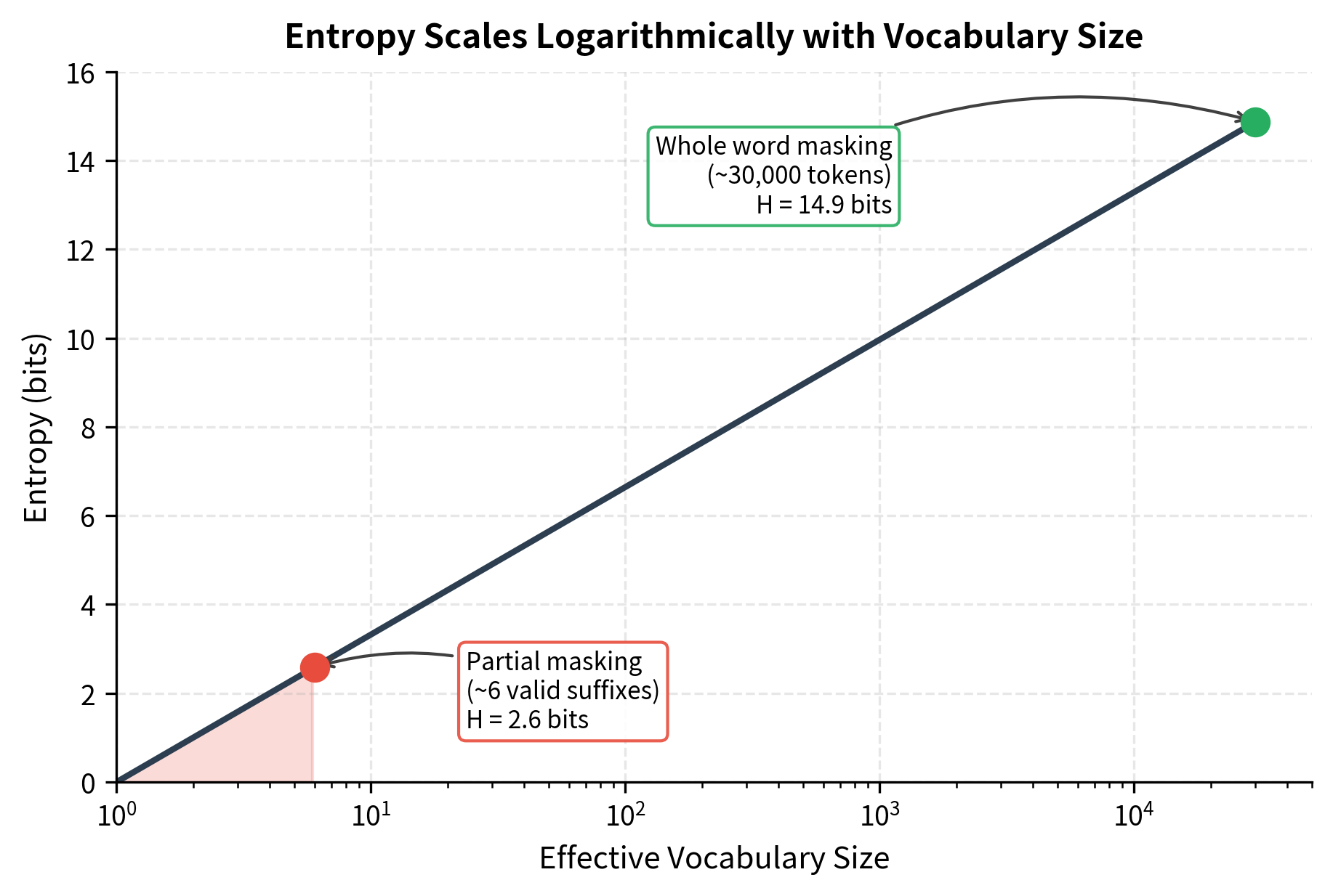
The visualization shows how dramatically entropy drops when the effective vocabulary shrinks. Partial masking constrains predictions to just a few valid suffixes, collapsing entropy from nearly 15 bits to around 2.6 bits. This 5-6x reduction in uncertainty means the model can achieve low loss without deep contextual understanding.

Why partial masking destroys the training signal

Now we can quantify the information leakage problem. When "transform" is visible and we mask only "##ation", what happens to the entropy?

The visible prefix constrains the possibilities dramatically. The only valid continuations are tokens that can follow "transform-" in English words: {##ation, ##ed, ##ing, ##er, ##s, ##able}. The effective vocabulary shrinks from 30,000 to perhaps 6 options. Even with a uniform distribution over these 6, entropy drops from 15 bits to about 2.6 bits.

In practice, it's even worse. The model learns that ##ation is by far the most common suffix after "transform-", so $P(\texttt{\#\#ation})$ might be 0.7 or higher. The entropy collapses further, perhaps to 1-2 bits.

This explains why partial masking produces weak gradients. The model achieves low loss not by understanding context, but by memorizing subword co-occurrence patterns. It learns morphology instead of semantics.

Whole Word Masking preserves word boundaries during the masking process. The algorithm requires knowing which subword tokens belong to the same original word. Different tokenizers signal this differently: WordPiece uses ## prefixes for continuation tokens, SentencePiece uses special Unicode characters, and BPE can use space prefixes.

The WWM procedure works in three steps:

1. Group subwords into words: Traverse the token sequence and collect consecutive subword tokens that belong to the same word. A new word starts when a token lacks the continuation marker.

2. Select words for masking: Choose words (not tokens) to mask based on the masking probability. The selection targets approximately 15% of the total tokens while operating at the word level.

3. Mask all subwords together: For each selected word, replace all its constituent subword tokens with [MASK].

The key insight is that we're changing the unit of selection from subword tokens to whole words while maintaining approximately the same masking ratio in terms of total tokens masked.

Standard MLM masks 15% of tokens. With WWM, we shift from selecting individual tokens to selecting whole words, but we still want approximately 15% of tokens to end up masked. This creates an interesting problem: words have different lengths in subword tokens.

The variable-length complication

Consider a concrete example. You have a sentence with 20 tokens forming 10 words:

• 6 words are single tokens (like "the", "is", "a")
• 3 words are two tokens each (like "trans##form", "learn##ing")
• 1 word is four tokens (like "un##believ##ab##ly")

If you randomly select 15% of words (1-2 words), you might mask anywhere from 1 token (if you pick "the") to 4 tokens (if you pick the long word). The actual token masking ratio becomes unpredictable: sometimes 5%, sometimes 20%.

A length-weighted selection approach

One solution weights word selection by length. The probability of masking each word becomes proportional to how many tokens it contributes:

where:

• $P(\text{mask word } w)$: the probability of selecting word $w$ for masking
• $|w|$: the number of subword tokens in word $w$
• $\sum_{i} |w_i|$: the total number of subword tokens in the sentence (summed across all words)
• $0.15$: the target masking ratio

The formula works by giving each word a selection probability proportional to its token count. A 4-token word is four times more likely to be selected than a 1-token word. This compensates for the fact that selecting the long word contributes four times as many masked tokens.

Why this approach has drawbacks

The length-weighted approach achieves precise 15% token masking on average, but it introduces a bias: longer words get masked more often. Since longer words tend to be rarer and more complex (like "internationalization" or "photosynthesis"), the model sees these words masked disproportionately often. It might develop weaker representations for common short words.

The practical solution

Production implementations typically use a simpler greedy approach:

1. Shuffle the list of words randomly
2. Add words to the masking set one by one
3. Stop when the total masked tokens reaches approximately 15%

This method is unbiased across word lengths and easy to implement. The masking ratio varies slightly per sentence (sometimes 12%, sometimes 18%), but these variations average out across a training batch. The model's performance is robust to this variance.

BERT's original masking strategy applies a probabilistic treatment to selected tokens:

• 80%: Replace with [MASK]
• 10%: Replace with a random token
• 10%: Keep the original token

With WWM, this rule extends to word boundaries. If a word is selected for the "random replacement" 10%, all its subwords are replaced with random tokens. If selected for the "keep original" 10%, all subwords remain unchanged. This maintains consistency within word boundaries.

Let's implement whole word masking step by step. We'll start with the core logic for identifying word boundaries, then build the complete masking function.

The first task is grouping subword tokens into words. WordPiece tokenizers mark continuation tokens with a ## prefix:

The function correctly identifies word boundaries by detecting the ## prefix. "The" remains a single-token word, while "transformation" is grouped as ["transform", "##ation"] and "undeniably" as ["undeni", "##ably"]. Each tuple represents the start and end indices in the token list, making it easy to mask all subwords of a word together.

Now we implement the complete WWM function. We'll select words for masking and apply the 80-10-10 rule:

The function masks entire words together. When "jumps" is selected, both "jump" and "##s" receive the same treatment. The labels array stores the original token IDs for computing the loss, with -100 marking positions to ignore.

Let's visualize the difference between random subword masking and WWM on a longer example:

In random subword masking, you might see "transform" with "##ational" masked, revealing the word structure. In WWM, the entire word is hidden.

Let's create a visualization comparing how both masking strategies affect a set of sentences:

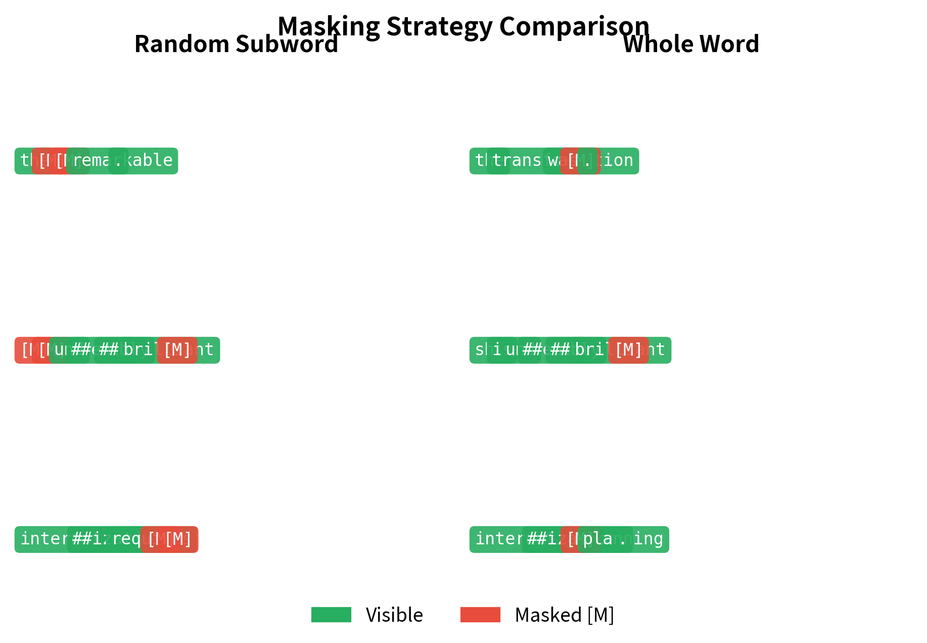
The visualization highlights how random subword masking creates fragmented masking patterns. In "transformation", you might see "transform" while "##ation" is masked. WWM eliminates this by treating words as atomic units.

Different tokenizers use different conventions for marking subword boundaries. Implementing WWM correctly requires adapting to each convention.

WordPiece uses ## to prefix continuation tokens. A word starts with a token lacking ##, and subsequent ##-prefixed tokens continue it:

SentencePiece uses the special character ▁ (U+2581) to mark word boundaries. Unlike WordPiece, this character appears at the start of words, not as a continuation marker:

GPT-2's BPE tokenizer uses a different convention: it adds Ġ (representing a space) at the start of tokens that begin a new word:

We can create a universal function that detects the tokenizer type and applies the appropriate grouping:

Each tokenizer produces different subword splits, but the universal function correctly groups them into a single word. BERT uses ## prefixes, T5 uses ▁ at word starts, and GPT-2 uses Ġ. The grouping result of [(0, n)] indicates all tokens belong to one word, exactly what we need for whole word masking.

Let's compare the prediction difficulty under both masking strategies. We'll measure how much information leakage helps the model make correct predictions:

The results demonstrate the information leakage problem. When "transform" is visible, predicting "##ation" is trivial since the model essentially pattern-matches to complete the word. When the entire word is masked, the model must genuinely reason about context to make predictions.

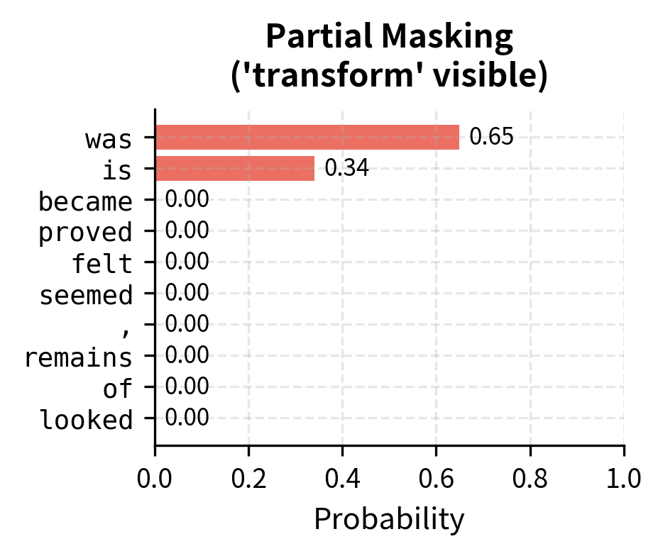
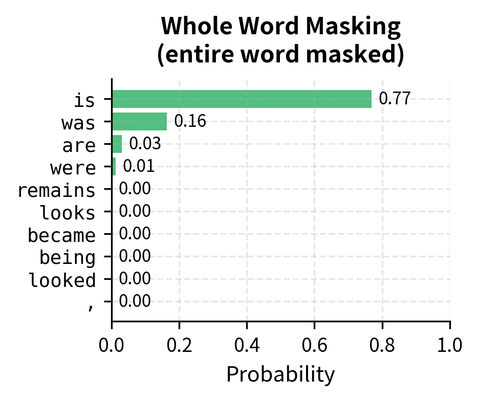
The contrast is striking. With partial masking, the model assigns overwhelming probability to ##ation because it simply completes the visible prefix. With whole word masking, the model must consider what noun could fit the context "The [MASK] was remarkable," leading to a more diverse and uncertain prediction. This uncertainty creates stronger gradients during training.

We can quantify the difficulty difference using prediction entropy:

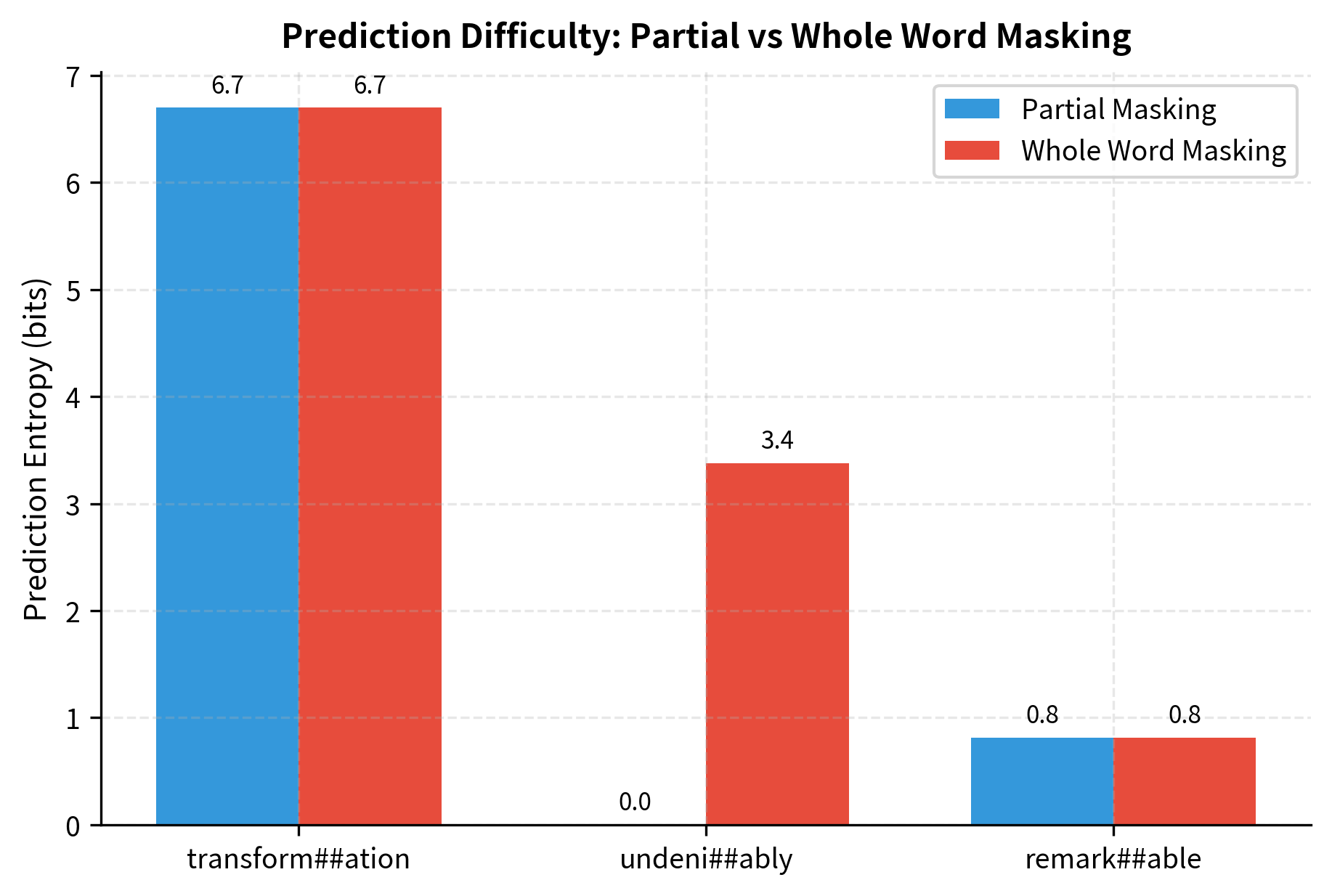
The entropy measurements confirm our intuition. Partial masking produces lower entropy predictions because the visible subword tokens constrain the answer. Whole word masking forces higher entropy, indicating a more challenging prediction task that requires deeper contextual understanding.

The Hugging Face transformers library provides built-in support for whole word masking through the DataCollatorForWholeWordMask class:

The output shows tensors with matching shapes for inputs and labels. The [MASK] tokens appear in the input sequence, while the labels tensor stores the original token IDs at those positions. Positions with -100 (shown as _) are ignored during loss computation, focusing training only on predicting the masked words.

To train a model with WWM, simply use the collator in your training pipeline:

The training loop applies WWM dynamically to each batch, ensuring different masking patterns on each epoch.

Whole word masking introduces trade-offs that practitioners should consider:

• Language-dependent effectiveness: WWM assumes that word boundaries carry semantic significance. This works well for English and other space-delimited languages, but languages without clear word boundaries (like Chinese or Japanese) require additional segmentation tools. For Chinese BERT models, word segmentation must happen before tokenization, adding complexity and potential error propagation.

• Inconsistent masking ratio: Because words have variable lengths in subword tokens, the actual percentage of tokens masked varies by sentence. A sentence with many long words might see 20% masking while one with short words sees 12%. This variance doesn't significantly harm training but differs from the precise 15% in standard MLM.

• Computational overhead: Identifying word boundaries adds preprocessing cost. For production training at scale, this overhead is negligible compared to model forward passes, but it complicates the data pipeline.

• Morphology complications: Some morphological processes don't respect word boundaries. In German, compound words like "Donaudampfschifffahrtsgesellschaft" might be tokenized into many subwords that all belong together semantically. WWM keeps them together, which might mask too large a chunk and provide insufficient learning signal.

Despite these limitations, WWM has proven valuable:

• Improved downstream performance: Google released BERT-wwm models showing improvements on SQuAD and other benchmarks. The gains are modest but consistent: typically 0.5-1.0 F1 points on reading comprehension tasks. For Chinese, the improvements are larger because character-level masking in standard BERT created severe information leakage.

• Better morphological understanding: WWM forces models to learn word-level rather than subword-level patterns. This produces representations that better capture morphological relationships. Words with shared roots cluster more meaningfully in the embedding space.

• Standard practice for non-English models: WWM has become the default for training BERT models in morphologically rich languages. German, Arabic, and especially Chinese BERT variants almost universally use WWM because the alternative loses too much training signal to information leakage.

• Foundation for span masking: WWM paved the way for more sophisticated masking strategies like span corruption in T5. The insight that masking units should respect linguistic boundaries generalizes beyond single words to phrases and sentences.

When implementing whole word masking, several parameters control the masking behavior:

• mlm_probability (default: 0.15): The target fraction of tokens to mask. WWM aims to achieve this ratio at the token level while selecting at the word level. Values between 0.1 and 0.2 work well; higher values provide more training signal per example but may make the task too difficult.

• mask_token: The special token used for masking (e.g., [MASK] for BERT). This must match the tokenizer's mask token exactly for the model to recognize masked positions.

• 80-10-10 distribution: Controls how selected tokens are modified. The standard split (80% [MASK], 10% random, 10% unchanged) helps bridge the gap between pre-training and fine-tuning, where [MASK] never appears.

• Word boundary detection: Different tokenizers require different detection logic:

  • WordPiece: Continuation tokens start with ##
  • SentencePiece: Word-initial tokens start with ▁
  • GPT-2 BPE: Word-initial tokens start with Ġ

• random_state / seed: Setting a seed ensures reproducible masking patterns during evaluation or debugging. During training, avoid fixed seeds to maximize data diversity across epochs.

Whole Word Masking addresses a fundamental flaw in applying masked language modeling to subword-tokenized text. When subword tokens are masked independently, visible sibling tokens leak information about masked positions, reducing the prediction task to pattern matching rather than contextual reasoning.

WWM's key contributions:

• Preserves word boundaries: All subwords of a word are masked together, eliminating within-word information leakage.

• Strengthens learning signal: The model must predict complete words from context alone, developing deeper semantic understanding.

• Adapts to tokenizer conventions: Different tokenizers mark word boundaries differently (##, ▁, Ġ), and WWM implementations must detect and handle each convention.

• Integrates with existing frameworks: Libraries like Hugging Face provide ready-to-use WWM data collators that handle all implementation details.

The technique is particularly important for languages with rich morphology and for any application where word-level understanding matters more than subword pattern matching. While the improvements over standard MLM are modest for English, they compound with other techniques and become essential for many non-English languages.

The next chapter explores span corruption, which extends the WWM insight further by masking contiguous spans of multiple words, creating even more challenging prediction tasks that encourage models to learn longer-range dependencies.

Ready to test your understanding? Take this quick quiz to reinforce what you've learned about Whole Word Masking.