

Master BERT fine-tuning for downstream NLP tasks. Learn task-specific heads, hyperparameter tuning, and strategies to prevent catastrophic forgetting.

This article is part of the free-to-read Language AI Handbook
Choose your expertise level to adjust how many terms are explained. Beginners see more tooltips, experts see fewer to maintain reading flow. Hover over underlined terms for instant definitions.
BERT Fine-tuning
You have a pre-trained BERT model with 110 million parameters trained on billions of words. Now you need it to classify movie reviews, identify named entities, or answer questions about documents. How do you adapt this general language understanding to your specific task?
Fine-tuning is the answer. Rather than training from scratch, you take BERT's pre-trained weights and continue training on your task-specific data. The model already understands language; fine-tuning teaches it your particular task. This chapter covers the complete fine-tuning process: how to add task-specific heads for classification, sequence labeling, and question answering; how to set hyperparameters that balance learning speed against stability; and how to avoid catastrophic forgetting, where the model loses its pre-trained knowledge.
The Fine-tuning Paradigm
Pre-training teaches BERT general language understanding. Fine-tuning specializes that understanding for downstream tasks. The key insight is that most of BERT's learned representations transfer well across tasks, so only minor adjustments are needed.
The process of taking a pre-trained model and continuing training on task-specific data with a task-specific objective. Fine-tuning updates all or most of the model's parameters, adapting general representations to the target task while preserving useful pre-trained knowledge.
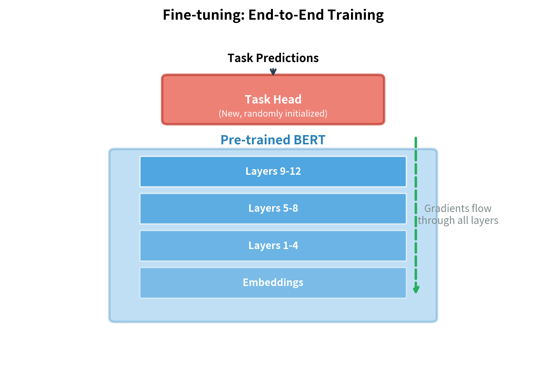
The fine-tuning workflow follows a consistent pattern:
- Load a pre-trained BERT model
- Add a task-specific head (classifier, token labeler, or span predictor)
- Train on labeled task data with a much lower learning rate than pre-training
- The entire model updates: both the new head and BERT's existing weights
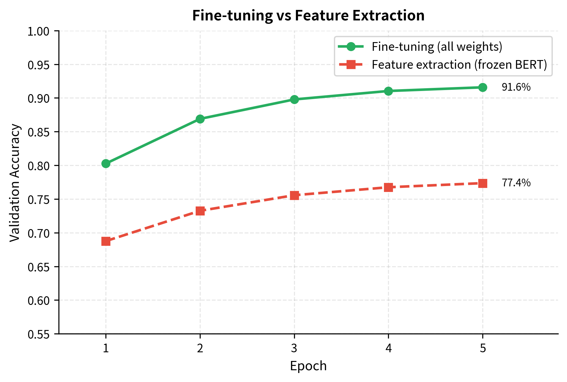
This differs from feature extraction, where BERT's weights are frozen and only the task head trains. Fine-tuning typically achieves better performance because BERT can adapt its internal representations to the task, not just learn to use fixed features.
Classification Fine-tuning
Sentiment analysis, spam detection, topic classification: these tasks require mapping an entire text to a single label. BERT handles classification through its [CLS] token.
The Classification Architecture
To classify a sentence, we need to reduce BERT's variable-length sequence of token representations into a single fixed-size vector. But which tokens should we use? We could average all token representations, but that treats every word equally, giving "the" as much weight as "terrible" in a movie review. We could use the final token, but that's arbitrary.
BERT's solution is elegant: it reserves a special [CLS] token at the beginning of every input specifically for sequence-level tasks. During pre-training, this token learned to aggregate information from the entire sequence for the Next Sentence Prediction objective. By the time pre-training finishes, the [CLS] representation has become a 768-dimensional summary of the sequence's meaning.
For classification, we add a single linear layer on top of this representation. The layer transforms the 768-dimensional [CLS] vector into a vector of class scores:
where:
- : the output logits vector with dimension (number of classes)
- : the weight matrix of shape that projects the hidden state to class space
- : the 768-dimensional hidden state of the
[CLS]token from BERT's final layer - : the bias vector of dimension
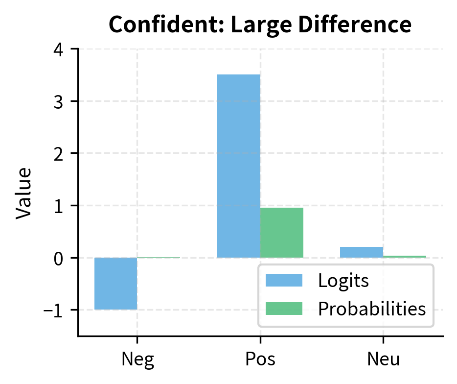
Each element of represents the model's confidence that the input belongs to that class, called a logit or unnormalized score. Higher values mean higher confidence. To convert these logits into proper probabilities that sum to 1, we apply the softmax function. During training, we minimize the cross-entropy loss between these predicted probabilities and the true labels, which pushes the model to assign high probability to the correct class and low probability to incorrect ones.
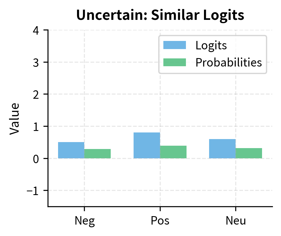
The probabilities are nearly equal, which is expected: the classifier produces random predictions because its weights are randomly initialized. BERT's layers contain useful pre-trained representations, but the classifier hasn't learned to use them yet. After fine-tuning on labeled sentiment data, these probabilities would reflect meaningful predictions.
Training Loop for Classification
Fine-tuning requires careful attention to learning rates, batch sizes, and training duration. Here's a complete training loop:
The decreasing training loss indicates the model is learning from the examples. Even with only 10 training examples and 2 epochs, the model begins adapting to the sentiment classification task. Real fine-tuning uses thousands of examples and typically runs for 3-4 epochs, achieving much stronger validation accuracy.
Multi-class Classification
The same architecture handles multi-class classification by changing the number of output classes:
The predictions are random because the model is untrained. The architecture remains identical to binary classification; only the output dimension changes from 2 to 4 classes. The softmax over 4 classes produces a probability distribution over topics. After fine-tuning on topic-labeled data, the model would correctly classify each text into its appropriate category.
Sequence Labeling Fine-tuning
Named Entity Recognition (NER), part-of-speech tagging, and similar tasks require predictions for each token, not just the sequence. Instead of using only the [CLS] token, we classify every token position.
Token Classification Architecture
Classification uses a single representation, the [CLS] token, to make one prediction for the entire sequence. But what if we need a prediction for every token? In Named Entity Recognition, each word gets a label: "John" is a person, "Google" is an organization, "works" is outside any entity. The model must make as many predictions as there are tokens.
The solution extends naturally from classification. Instead of applying our linear layer only to [CLS], we apply the same linear transformation to every token's representation. For each position in the sequence:
where:
- : the logits for position with dimension (number of labels)
- : the hidden state at position from BERT's final layer
- : the shared weight matrix of shape applied to all positions
- : the shared bias vector
An important design choice: we use the same and for every position. This weight sharing makes sense because the meaning of labels doesn't change across positions: a "person" label means the same thing whether we're classifying the first token or the tenth. Sharing weights also keeps the parameter count manageable; without sharing, we'd need separate parameters for each possible position.
The output is a matrix of logits with shape (sequence_length, num_labels). We apply softmax independently to each row to get per-token probability distributions, then take the argmax to get the predicted label for each position:
The predicted labels are random because the classifier weights haven't been trained. In a trained NER model, "John" and "Smith" would receive B-PER and I-PER tags, "Google" would receive B-ORG, and "California" would receive B-LOC. The O (Outside) tag would correctly mark non-entity tokens like "works" and "at".
Handling WordPiece Tokenization
A subtle challenge arises from WordPiece tokenization. When a word splits into multiple subwords, which subword's prediction should we use?
The word "unbelievable" tokenizes into multiple subwords (likely "un", "##believ", "##able"). The alignment function takes the first subword's prediction as the label for the entire word. This is necessary because NER labels apply to words, not subwords. Alternative strategies include averaging logits across subwords or using the last subword's prediction.
The IOB Tagging Scheme
NER commonly uses Inside-Outside-Beginning (IOB) tagging. "B-" marks the beginning of an entity, "I-" continues it, and "O" marks non-entity tokens.
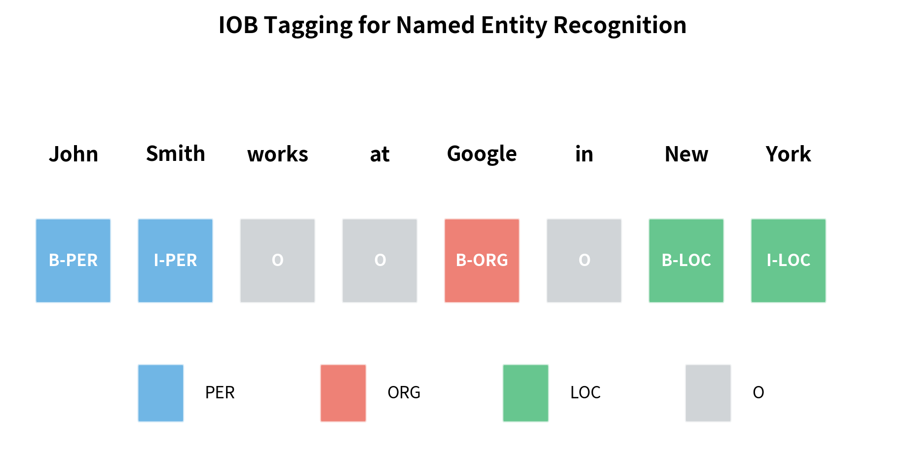
The IOB scheme allows multi-word entities: "John Smith" spans two tokens with B-PER and I-PER, while "New York" spans B-LOC and I-LOC. This is why sequence labeling is more complex than simple classification: the model must learn to produce coherent tag sequences.
Question Answering Fine-tuning
Extractive question answering finds answer spans within a context passage. Given a question and context, the model predicts which tokens constitute the answer.
Span Prediction Architecture
Question answering presents a fundamentally different challenge from classification or sequence labeling. The answer to a question isn't a single label but a contiguous span of text within the context. For "Where does John work?", the answer "Google" is a substring of the passage. We need to predict both where this substring starts and where it ends.
Consider the alternatives. We could treat this as token classification, labeling each token as "in answer" or "not in answer." But this approach has a flaw: it doesn't guarantee a contiguous span. The model might label disconnected tokens as part of the answer. We could add constraints, but there's a simpler approach.
Instead of classifying each token, we compute two scores: how likely each position is to be the answer's start, and how likely each position is to be the answer's end. For each token position :
where:
- : the start score for position (higher means more likely to be the answer start)
- : the end score for position (higher means more likely to be the answer end)
- : the learned weight vector for start prediction (768 dimensions)
- : the learned weight vector for end prediction (768 dimensions)
- : the hidden state at position from BERT's final layer
Notice that these are dot products, not full linear layers. Each score is a simple weighted sum of the hidden state dimensions. We use separate weight vectors and because the features that indicate "this is where an answer starts" differ from those indicating "this is where an answer ends."
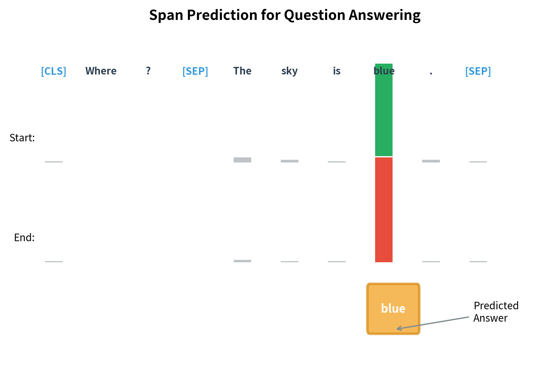
The predicted answer span is the substring from position to position . We find the token with the highest start score and the token with the highest end score, then extract everything between them (inclusive). During inference, we add a constraint: the end position must not precede the start position.
The predicted positions are random because the span prediction heads haven't been trained. In a fine-tuned model, the start position would point to "Google" and the end position would also point to "Google" (or to "California" if the question asked about location). The model learns to identify answer boundaries by training on question-context-answer triplets from datasets like SQuAD.
The SQuAD Format
The Stanford Question Answering Dataset (SQuAD) is the standard benchmark for extractive QA. Each example contains a context paragraph, a question, and the answer's start position in the context.
The answer "blue" was correctly located at token positions within the context. During training, these start and end positions serve as labels: the model learns to maximize the probability of the correct positions. The key challenge is aligning character-level answer positions to token-level positions. The offset_mapping from the tokenizer provides this alignment, mapping each token to its character span in the original text.
Unanswerable Questions
SQuAD 2.0 introduced unanswerable questions: the answer might not exist in the context. To handle this, the model can predict the [CLS] position as both start and end, indicating "no answer."
Fine-tuning Hyperparameters
Fine-tuning is sensitive to hyperparameter choices. Unlike pre-training, where you have billions of tokens, fine-tuning datasets are often small (thousands of examples), making overfitting a constant concern.
Learning Rate
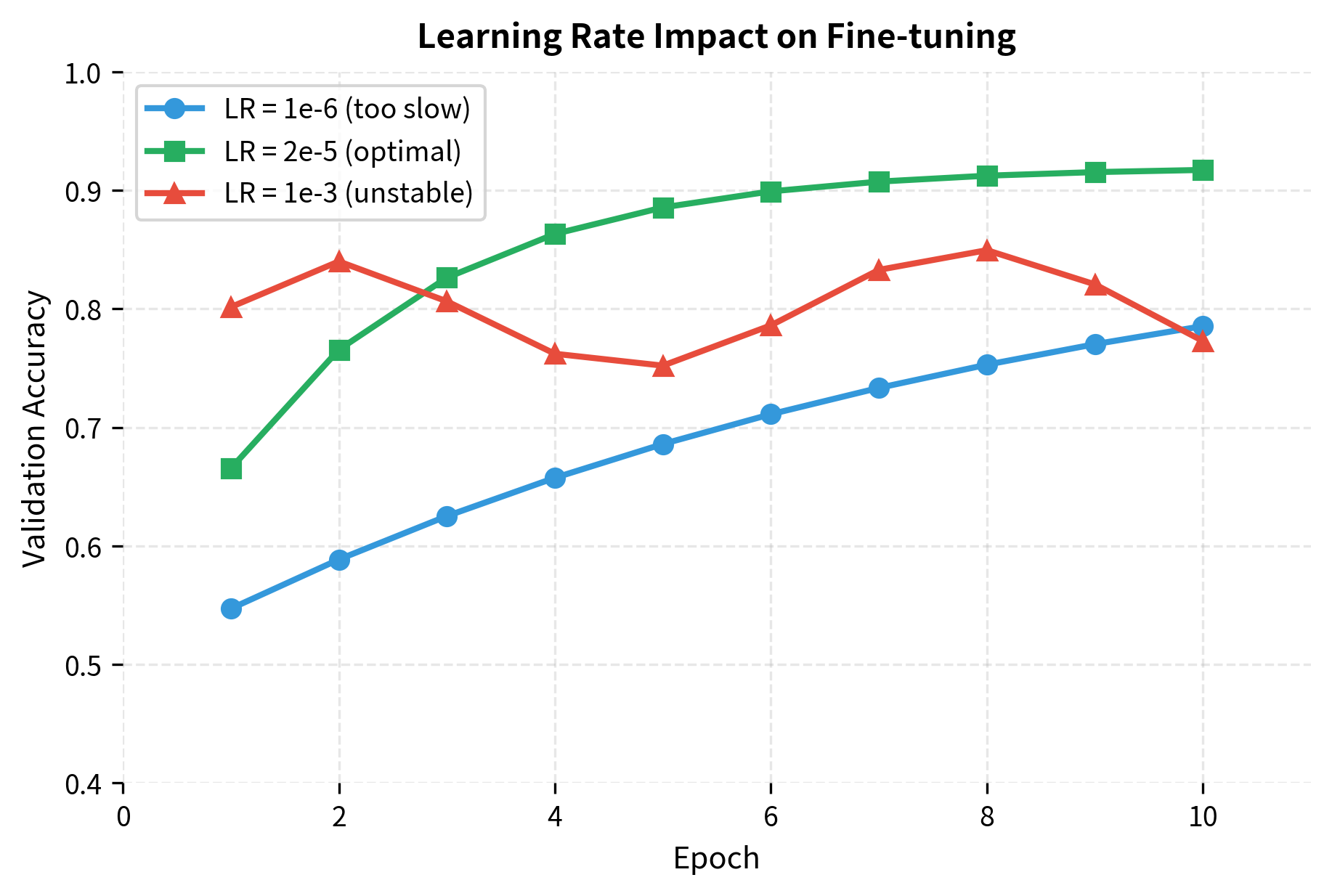
The learning rate is the most critical hyperparameter. BERT's original paper recommends values in the range 2e-5 to 5e-5, much smaller than typical neural network training.
Pre-trained weights encode valuable knowledge. Large learning rates would rapidly overwrite this knowledge with task-specific but potentially less general patterns. Small learning rates allow gradual adaptation while preserving useful representations.
Batch Size and Training Steps
BERT fine-tuning typically uses batch sizes of 16 or 32. Larger batches can work with learning rate scaling, but smaller datasets may not benefit.
Training duration is measured in epochs. Most tasks converge within 2-4 epochs. More epochs risk overfitting, especially on small datasets.
Smaller datasets benefit from smaller batch sizes (16) to see more gradient updates per epoch, and more epochs (4) to learn from limited data. Larger datasets can use bigger batches (32) for stability and fewer epochs (3) since each epoch provides more learning signal. The total steps column shows how training duration scales with dataset size.
Warmup and Learning Rate Scheduling
Why not just use a constant learning rate? Two problems arise. First, in early training, the classifier head's weights are random, producing random gradients that might destabilize BERT's carefully tuned representations. Second, in late training, the model is close to convergence, and large updates can overshoot the optimum.
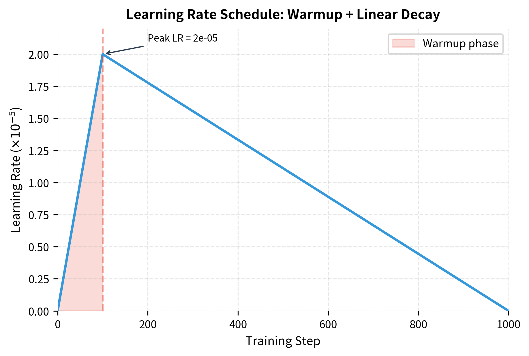
Learning rate scheduling addresses both problems by varying the learning rate throughout training. The standard BERT schedule has two phases:
-
Warmup: The learning rate starts at zero and increases linearly to its peak value. This gives the classifier time to produce meaningful gradients before larger updates hit BERT's layers.
-
Linear decay: The learning rate decreases linearly from its peak to zero. This allows fine-grained adjustments as the model converges.
The complete schedule can be expressed mathematically as:
where:
- : the learning rate at step
- : the maximum learning rate (typically 2e-5 to 5e-5 for BERT)
- : the number of warmup steps (typically 10% of total steps)
- : the total number of training steps
Let's trace through the schedule. At step 0, : the model doesn't update at all. By step , the learning rate reaches its peak: . Then it begins declining, reaching zero exactly at step . The denominator in the decay phase ensures the linear decrease is calibrated to hit zero at the final step.
Layer-wise Learning Rate Decay
So far, we've treated all of BERT's parameters equally: every layer receives the same learning rate. But should they? Research on transfer learning suggests that different layers encode different kinds of information:
- Lower layers (near the input) encode general linguistic features: part-of-speech patterns, syntactic structures, word relationships. These are useful across many tasks.
- Upper layers (near the output) encode more abstract, task-specific features. In pre-training, these became tuned to masked language modeling and next sentence prediction.
For fine-tuning, this layered structure suggests a strategy: preserve the general features in lower layers by updating them slowly, while allowing upper layers to adapt more aggressively to the new task. We can implement this by giving each layer its own learning rate, with lower layers receiving smaller rates.
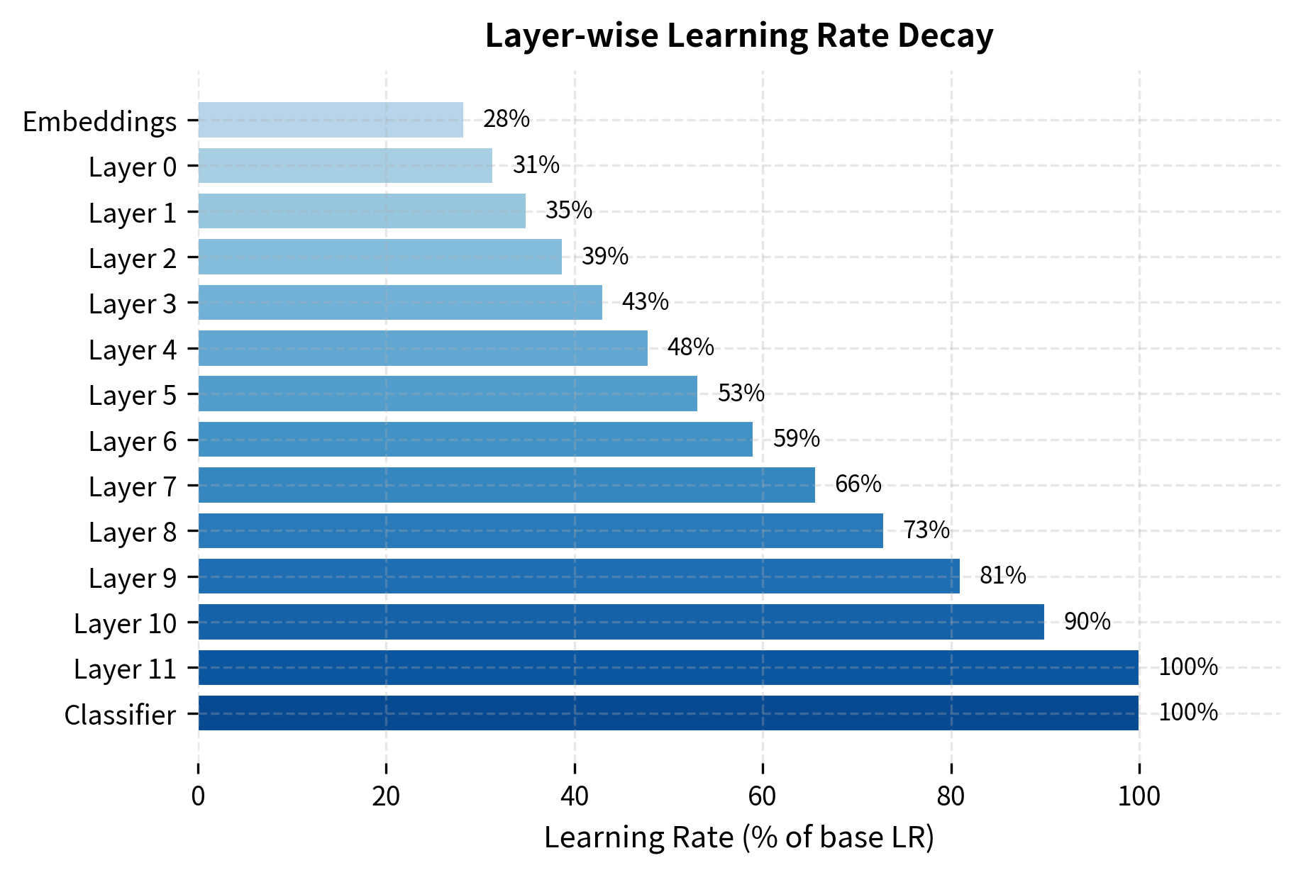
The pattern is clear: the embeddings, which encode the most fundamental token representations, receive the smallest learning rate (about 28% of the base). Each successive layer receives a slightly higher rate, culminating in the classifier head, which gets the full base learning rate since it must learn entirely from scratch.
The layer-wise learning rate for layer (counting from 0 at the bottom) is computed as:
where:
- : the learning rate for layer
- : the base learning rate (used for the classifier)
- : the decay rate (typically 0.9 or 0.95)
- : the total number of transformer layers (12 for BERT-Base)
Let's unpack this formula. The exponent counts how many layers are above layer . For the top layer (layer 11 in BERT-Base), , so : it gets the full learning rate. For layer 10, : it gets 90% of the full rate. For layer 0 (the bottom transformer layer), : it gets about 31% of the full rate.
The embeddings sit below all transformer layers. By convention, they receive . This 28% rate reflects how important it is to preserve the token embeddings that encode fundamental word meanings.
Catastrophic Forgetting
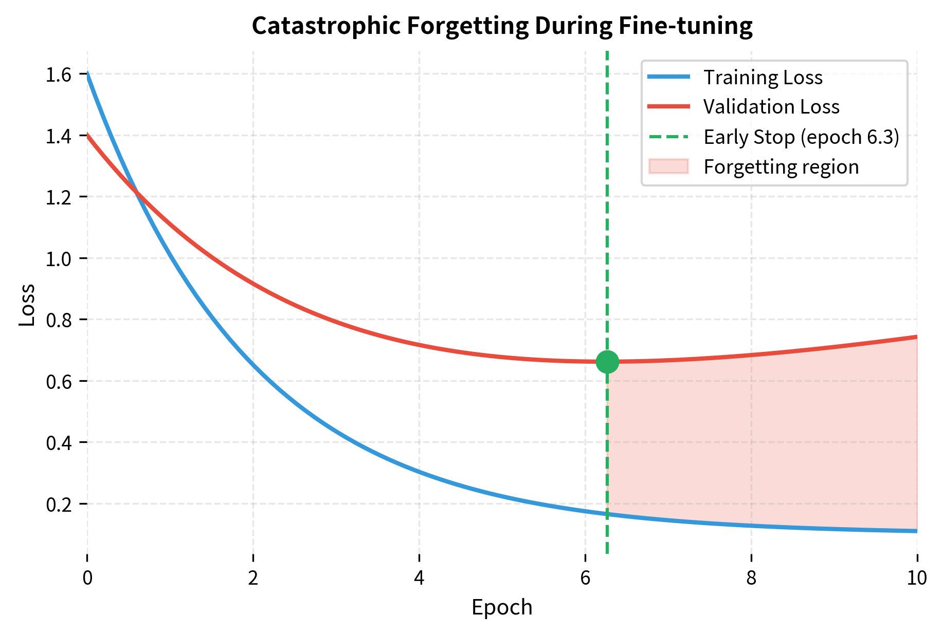
Catastrophic forgetting occurs when fine-tuning overwrites the general knowledge BERT learned during pre-training. The model becomes highly specialized for the fine-tuning task but loses its ability to generalize.
The phenomenon where a neural network, when trained on a new task, rapidly forgets previously learned information. In the context of BERT fine-tuning, this means losing pre-trained language understanding while adapting to a specific downstream task.
Signs of Catastrophic Forgetting
Several symptoms indicate catastrophic forgetting:
- Validation loss increases after initial decrease
- Out-of-domain performance drops on examples unlike the training data
- Model becomes overconfident on training-like examples but fails on variations
- Pre-training task performance degrades (masked language modeling accuracy drops)
Prevention Strategies
Several techniques mitigate catastrophic forgetting:
1. Use small learning rates: The most important factor. Rates of 2e-5 to 5e-5 allow gradual adaptation.
2. Train for few epochs: 2-4 epochs is typically sufficient. More epochs increase forgetting risk.
3. Early stopping: Monitor validation loss and stop when it starts increasing.
4. Regularization: Weight decay penalizes large weights, keeping them from growing unbounded. The AdamW optimizer applies weight decay directly to the weights:
where:
- : the model parameters at step
- : the learning rate
- , : bias-corrected first and second moment estimates from Adam
- : the weight decay coefficient (0.01 is standard for BERT)
- : small constant for numerical stability
The update has two parts. The first term is the standard Adam update, moving parameters in the direction that reduces loss. The second term shrinks every weight toward zero by a fraction proportional to its current magnitude. This shrinkage keeps weights close to their initial values, which for BERT means close to the pre-trained weights. The net effect: the model can adapt to the task, but large deviations from pre-training are penalized.
5. Layer freezing: Freeze lower BERT layers that encode general features, only fine-tuning upper layers.
Freezing the bottom 6 layers reduces trainable parameters by roughly half. This significantly decreases memory requirements and training time while preserving the general language understanding encoded in lower layers. The remaining trainable parameters in layers 6-11 and the classifier can still adapt to the task.
6. Mixout regularization: Randomly replace model weights with pre-trained weights during training, maintaining proximity to the original model.
Gradual Unfreezing
A sophisticated approach progressively unfreezes layers during training:
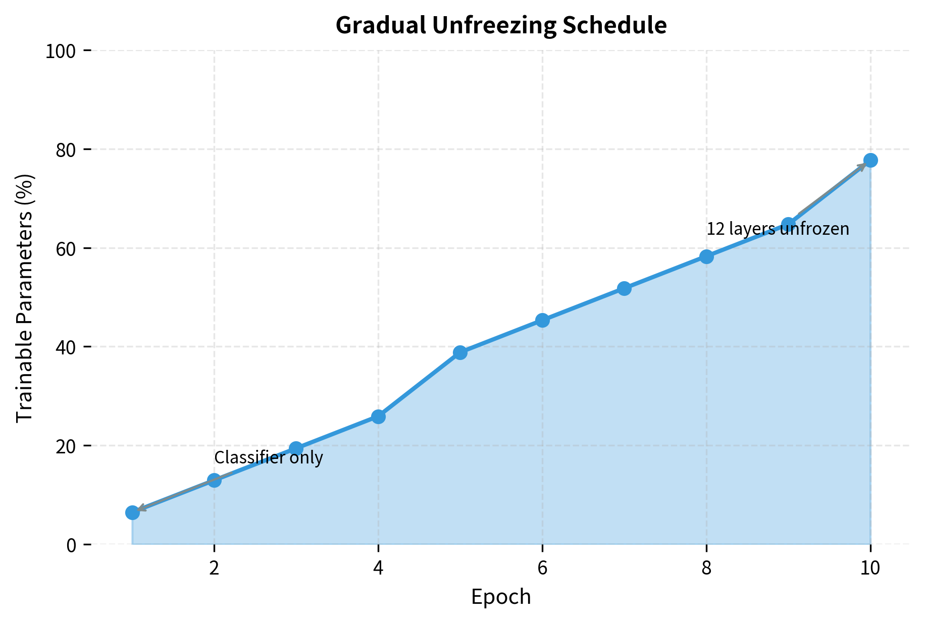
The schedule starts by training only the classifier head in early epochs, letting it adapt to the task while BERT's weights remain frozen. As training progresses, more transformer layers are unfrozen from the top (layer 11) down. By epoch 10, most layers are trainable. This gradual approach reduces forgetting risk because the classifier establishes useful gradients before deeper layers begin updating.
Practical Recommendations
Successful fine-tuning requires balancing several factors. Here are concrete recommendations based on the original BERT paper and subsequent research.
Standard Recipe
For most classification and sequence labeling tasks:
| Parameter | Recommended Value |
|---|---|
| Learning rate | 2e-5 to 5e-5 |
| Batch size | 16 or 32 |
| Epochs | 2-4 |
| Warmup ratio | 10% of total steps |
| Weight decay | 0.01 |
| Max sequence length | 128-512 (task-dependent) |
| Dropout | 0.1 |
Dataset Size Guidelines
The amount of training data affects hyperparameter choices:
- Small datasets (< 1K examples): Use lower learning rates (1e-5), more epochs (4-5), and consider layer freezing
- Medium datasets (1K-10K examples): Standard settings work well
- Large datasets (> 10K examples): Can use larger learning rates (5e-5), fewer epochs (2-3)
Task-Specific Considerations
Different tasks benefit from different approaches:
Classification: Standard recipe works well. Focus on class imbalance if present.
Sequence labeling (NER, POS): Handle subword alignment carefully. Consider CRF layer on top for structured prediction.
Question answering: Use longer max sequence lengths (384-512). Handle impossible questions by allowing null predictions.
Sentence pair tasks: Leverage segment embeddings. Consider whether task requires symmetric (similarity) or asymmetric (entailment) modeling.
When Fine-tuning Fails
If results are poor, try these debugging steps:
- Check data quality: Are labels correct? Is the task well-defined?
- Try different learning rates: Run a sweep from 1e-5 to 5e-5
- Increase training data: Can you augment or synthesize examples?
- Use a different model size: BERT-Large may help for complex tasks
- Consider domain mismatch: Pre-train further on domain-specific data first
Limitations and Practical Considerations
Fine-tuning BERT has constraints that affect real-world deployment.
Compute requirements remain substantial. Fine-tuning BERT-Base requires a GPU with at least 16GB memory for reasonable batch sizes. Training takes hours even on modern hardware. For resource-constrained settings, consider DistilBERT or smaller variants.
Sequence length limits cap input at 512 tokens. Longer documents require chunking strategies, which may lose cross-chunk context. For document-level tasks, consider Longformer or hierarchical approaches.
Domain mismatch between pre-training data (Wikipedia, books) and target domain (medical, legal, code) may require continued pre-training before fine-tuning. Domain-specific BERT variants like BioBERT, LegalBERT, and CodeBERT address this for common domains.
Label imbalance in task data can skew the model toward majority classes. Use weighted loss functions, oversampling, or stratified batching to address imbalance.
Reproducibility is challenging due to the stochastic nature of fine-tuning. Small changes in random seeds, data order, or hyperparameters can cause significant performance variation. The original BERT paper reported high variance across runs on some tasks, recommending multiple runs with different seeds.
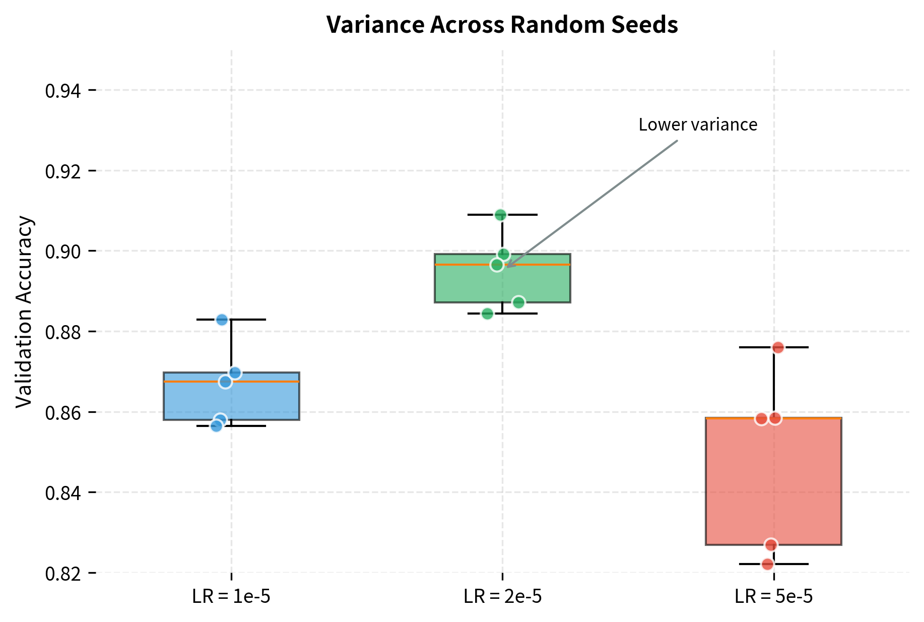
Despite these limitations, fine-tuning remains the most practical approach for adapting pre-trained models to specific tasks. The alternative, training from scratch, requires orders of magnitude more data and compute. Fine-tuning leverages the substantial investment already made in pre-training, allowing you to build effective models with limited task-specific resources.
Key Parameters
The most important hyperparameters for BERT fine-tuning:
-
learning_rate (2e-5 to 5e-5): Controls how quickly the model adapts. Too high causes instability and forgetting; too low learns too slowly. Start with 2e-5 for sensitive tasks, 5e-5 for robust ones.
-
num_epochs (2-4): Number of passes through the training data. More epochs increase forgetting risk. Use early stopping to find the optimal point.
-
batch_size (16-32): Number of examples per gradient update. Larger batches are more stable but require more memory. Gradient accumulation can simulate larger batches.
-
warmup_ratio (0.1): Fraction of training spent warming up the learning rate. Prevents early instability from noisy gradients.
-
weight_decay (0.01): L2 regularization coefficient. Penalizes large weight changes, helping preserve pre-trained knowledge.
-
max_length (128-512): Maximum sequence length after tokenization. Longer sequences require more memory and compute. Use the shortest length that captures your data.
-
dropout (0.1): Applied in the classifier head. Increase for small datasets to reduce overfitting.
-
gradient_clip (1.0): Maximum gradient norm. Prevents exploding gradients during training.
Summary
Fine-tuning adapts BERT's pre-trained knowledge to specific tasks through continued training on labeled data. The key insights for effective fine-tuning:
- Task heads map BERT outputs to task-specific predictions: classification uses
[CLS], sequence labeling uses all tokens, and QA predicts answer spans - Hyperparameters matter: Small learning rates (2e-5 to 5e-5), few epochs (2-4), and warmup prevent catastrophic forgetting while enabling task adaptation
- Catastrophic forgetting occurs when fine-tuning overwrites pre-trained knowledge. Prevent it with appropriate learning rates, early stopping, and layer freezing
- Layer-wise strategies like differential learning rates and gradual unfreezing provide fine-grained control over the adaptation process
- Practical constraints include compute requirements, sequence length limits, and domain mismatch, all of which have established solutions
Fine-tuning bridges the gap between general language understanding and specific applications. A single afternoon of fine-tuning can produce state-of-the-art results on tasks that would otherwise require months of data collection and model development. This efficiency is why BERT and its successors have become the default starting point for most NLP applications.
Quiz
Ready to test your understanding? Take this quick quiz to reinforce what you've learned about BERT fine-tuning.

Comments