

Learn how replaced token detection trains language models 4x more efficiently than masked language modeling by learning from every position, not just masked tokens.

This article is part of the free-to-read Language AI Handbook
Choose your expertise level to adjust how many terms are explained. Beginners see more tooltips, experts see fewer to maintain reading flow. Hover over underlined terms for instant definitions.
Replaced Token Detection
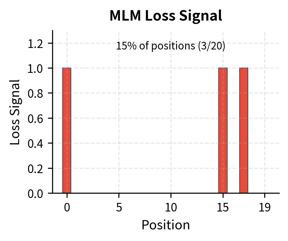
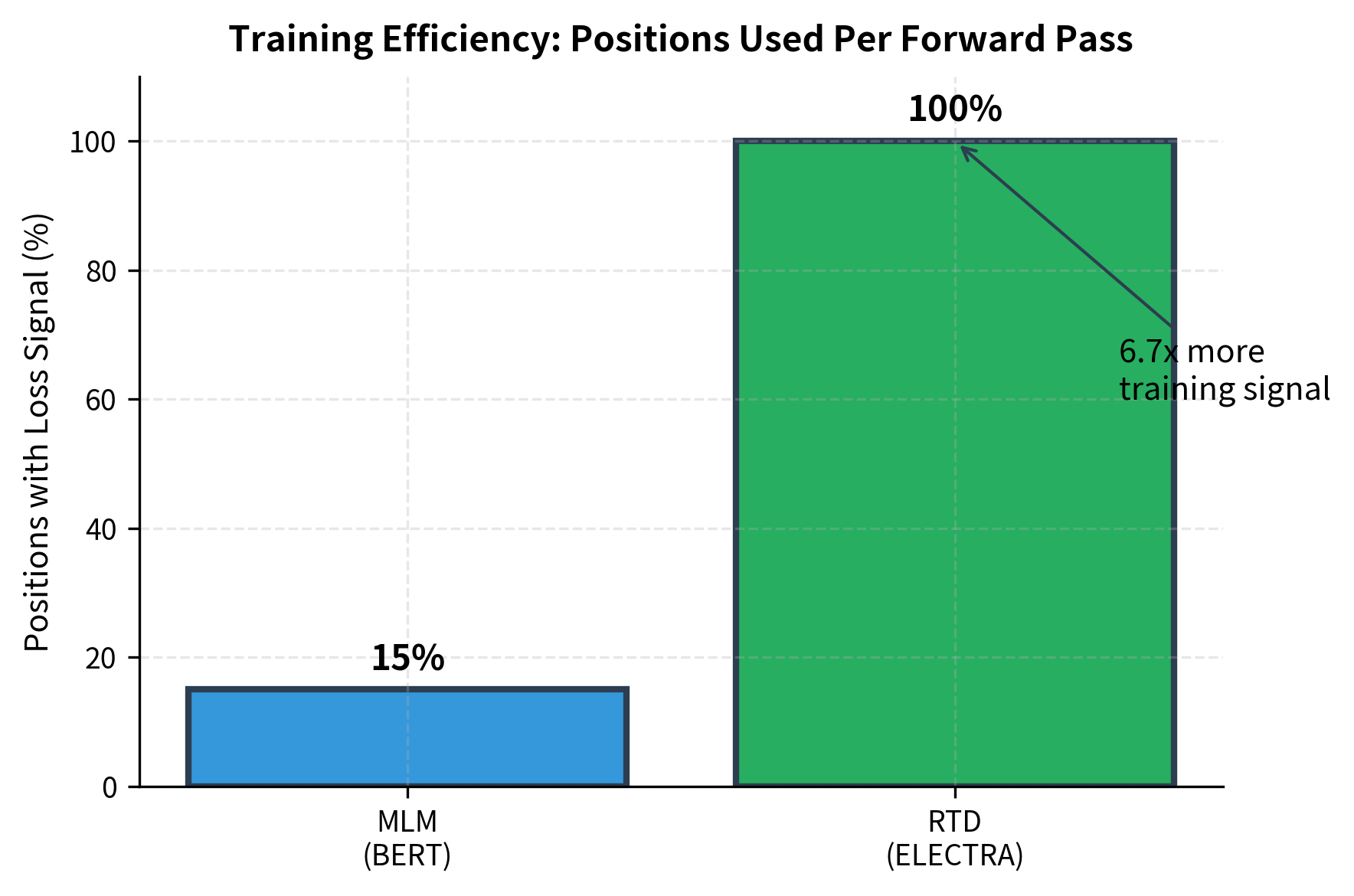
Masked language modeling wastes compute. When BERT masks 15% of tokens and predicts only those positions, 85% of the forward pass produces no training signal. The model processes the entire sequence but learns from a small fraction of it. For expensive pretraining runs consuming millions of GPU hours, this inefficiency is costly.
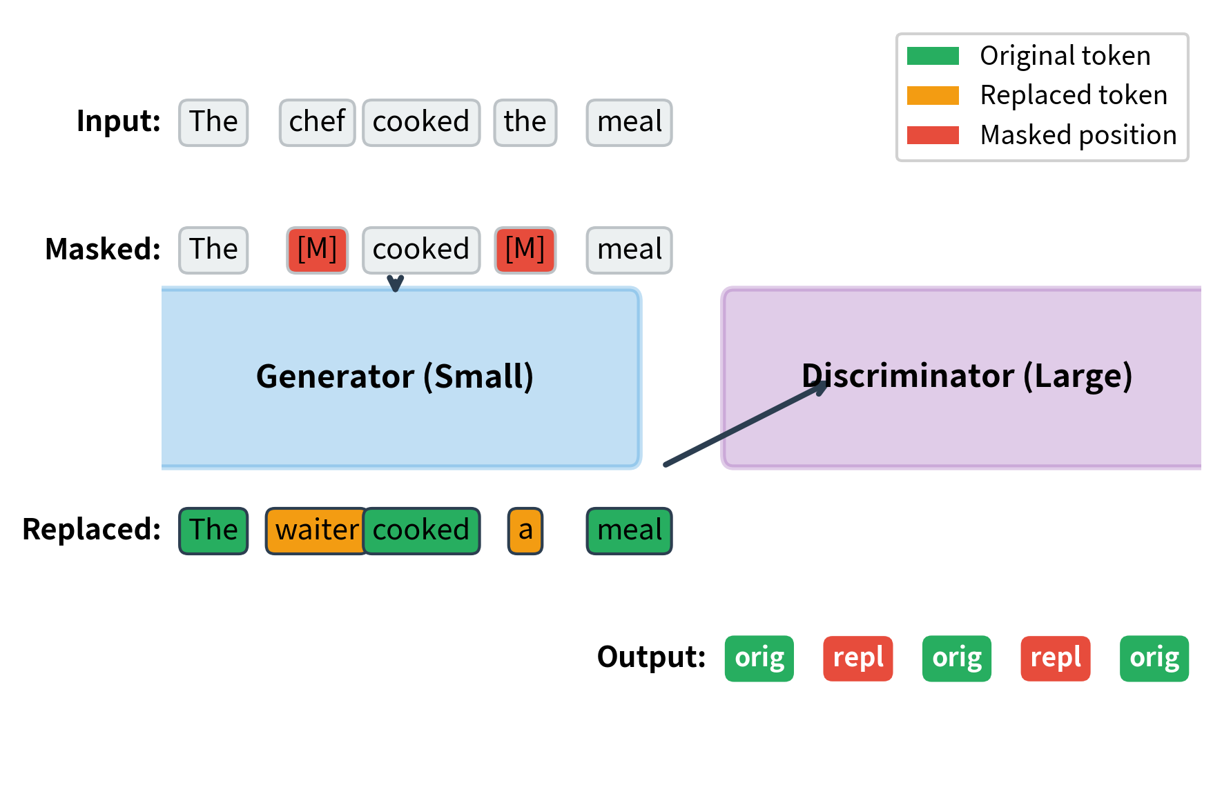
Replaced Token Detection (RTD) solves this problem with a different formulation. Instead of predicting masked tokens, the model classifies every token as either original or replaced. A small "generator" network produces plausible replacements for masked positions, and a larger "discriminator" network learns to detect which tokens have been swapped. Every position contributes to the loss, making training much more sample-efficient.
This approach, introduced in the ELECTRA paper in 2020, achieves BERT-level performance with a fraction of the compute. The key insight is that detection is easier than generation: distinguishing real from fake requires less capacity than predicting the exact original token, allowing the model to learn from every position rather than just masked ones.
The Generator-Discriminator Setup
RTD uses two networks working together: a small generator that creates replacements and a larger discriminator that detects them. This setup resembles generative adversarial networks (GANs) but with an important difference: training uses maximum likelihood, not adversarial objectives.
A pretraining objective where some tokens are replaced with plausible alternatives, and the model learns to classify each token as original or replaced. Unlike MLM, which predicts tokens only at masked positions, RTD produces a binary classification signal at every position, greatly improving sample efficiency.
The architecture works as follows. First, we mask some positions in the input sequence, exactly as in MLM. The generator, typically a small transformer, predicts tokens for the masked positions. We sample from the generator's output distribution to create replacement tokens. The discriminator, a larger transformer, receives the corrupted sequence and must identify which tokens were replaced.
The key point is that the generator and discriminator have different roles. The generator only needs to produce plausible replacements, not perfect ones. It can be small, perhaps one-quarter or one-third the size of the discriminator. The discriminator, which will be used for downstream tasks, receives the bulk of the parameters and learns rich representations from the detection task.
The RTD Objective
To understand how RTD trains both networks effectively, we need to think about what each network must learn and how to measure its progress. The generator must learn to produce plausible replacements for masked tokens, while the discriminator must learn to detect which tokens have been swapped. These are different tasks requiring different loss functions, yet they must work together in a single training loop.
Let's build up the complete objective by examining each component, understanding why it takes its particular form, and seeing how the pieces combine into an efficient training signal.
Generator Loss: Learning to Replace
The generator faces a familiar task: predict the original token at each masked position. This is identical to masked language modeling. We mask some positions in the input, show the generator the corrupted sequence, and ask it to predict what was hidden.
Why use MLM for the generator? The goal is to produce plausible replacements that will challenge the discriminator. A generator that simply outputs random tokens would be trivial to detect. By training on MLM, the generator learns the statistical patterns of language, producing replacements that fit grammatically and semantically into their contexts. The discriminator then must develop nuanced understanding to distinguish these plausible fakes from originals.
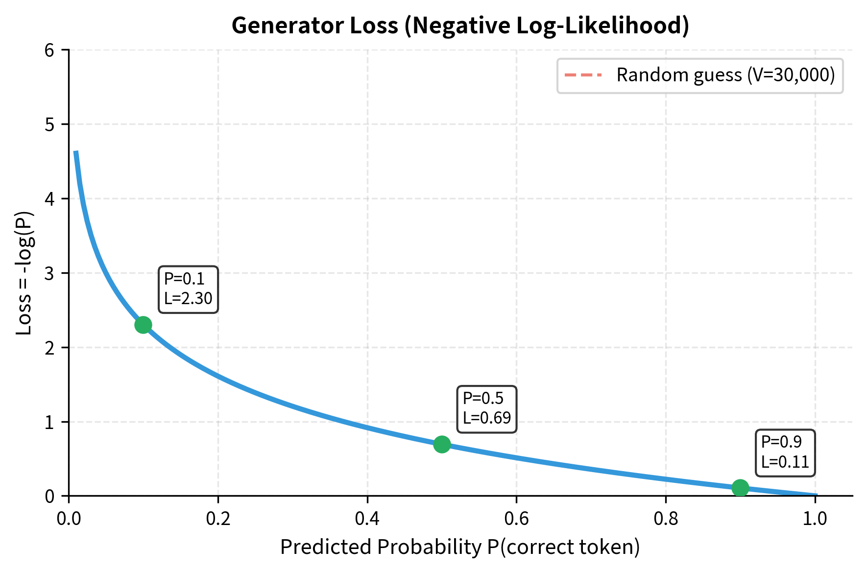
Formally, given a set of masked positions , we minimize the negative log-likelihood of the original tokens:
where:
- is the generator loss, identical to standard MLM loss
- is the set of masked position indices (typically 15% of positions)
- is the original token at position that we want to predict
- is the corrupted input sequence with
[MASK]tokens at positions in - is the probability the generator assigns to the correct token , conditioned on seeing the masked sequence
To understand this formula intuitively, consider what happens as training progresses. Initially, the generator assigns roughly uniform probability across all vocabulary tokens, making where is vocabulary size. The log of this small probability is a large negative number, producing high loss. As the generator learns, it concentrates probability on likely tokens, increasing toward 1. The log approaches zero, and loss decreases.
The summation iterates only over masked positions because those are the only positions where we have a prediction task. Unmasked positions pass through unchanged, contributing nothing to generator learning. This sparsity is the inefficiency that the discriminator's loss will address.
Discriminator Loss: Learning to Detect
Now we arrive at the key innovation. The discriminator receives a sequence where masked positions have been filled with generator samples, and must classify every token as original or replaced. This binary classification task applies to all positions, providing the dense training signal that makes RTD efficient.
Think about what the discriminator must learn. For original tokens, it needs to recognize that they fit naturally into their context. For replaced tokens, even plausible ones, it must detect subtle mismatches. Perhaps the replacement "waiter" in "The waiter barked loudly" is grammatically acceptable but semantically wrong. The discriminator learns these nuances by processing the entire sequence and making a decision at each position.
We create the corrupted sequence by sampling from the generator's output distribution at masked positions. The discriminator then outputs a probability for each position, and we compute binary cross-entropy against the ground truth labels:
where:
- is the discriminator loss, a sum over all positions
- is the total sequence length (not just masked positions)
- is the binary label at position (1 if original, 0 if replaced)
- is the corrupted sequence with generator samples inserted at previously masked positions
- is the discriminator's predicted probability that position contains an original token
This binary cross-entropy formula rewards correct predictions at both extremes. Let's trace through what each term contributes:
-
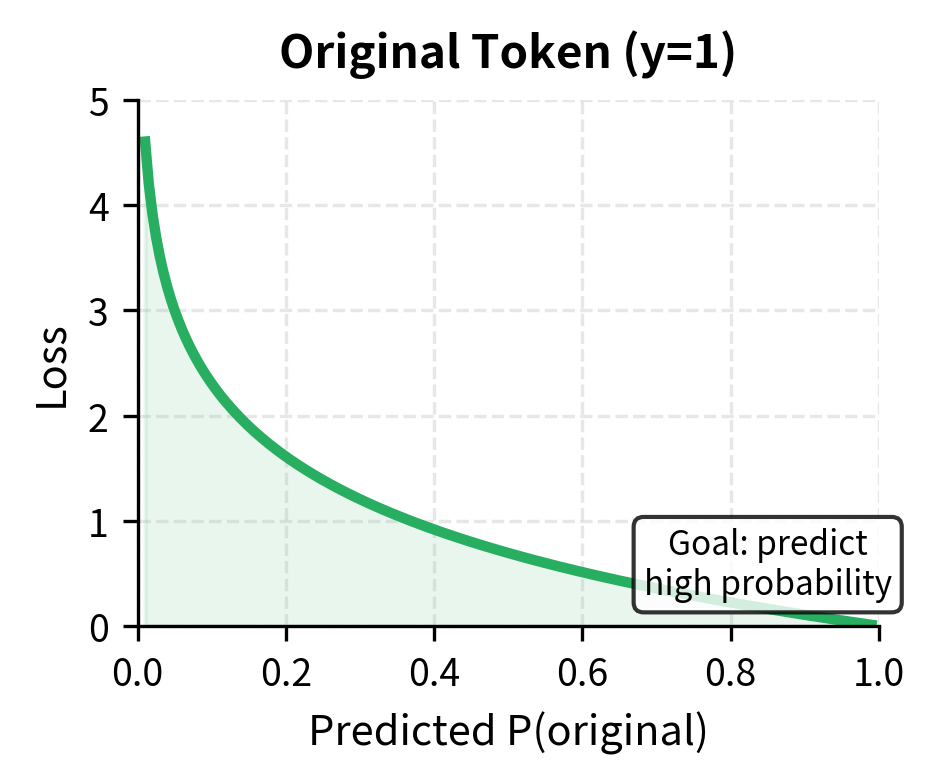
For original tokens (): The second term vanishes since . The loss becomes . When the discriminator correctly predicts high probability (near 1.0), the log is near zero, contributing little loss. When it incorrectly predicts low probability, the log is a large negative number, producing high loss.
-
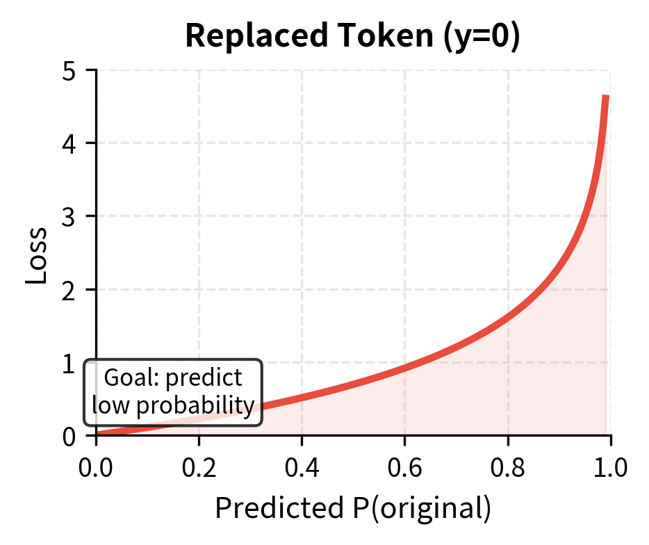
For replaced tokens (): The first term vanishes. The loss becomes . When the discriminator correctly predicts low probability (near 0), is near 1, and the log is near zero. When it incorrectly predicts high probability, the loss is large.
The key point is that this loss applies to every position in the sequence. Most positions contain original tokens, so the discriminator primarily learns what "normal" tokens look like in context. A small fraction contain replacements, teaching the discriminator what "wrong" looks like. Both types of positions contribute to learning, giving 6-7x more training signal than MLM's masked-only approach.
Combining the Losses
With both component losses defined, we need a strategy for combining them into a single objective that trains both networks. The simplest approach is a weighted sum:
where:
- is the total loss used to update both networks
- is the generator's MLM loss (computed only at masked positions)
- is the discriminator's binary classification loss (computed at all positions)
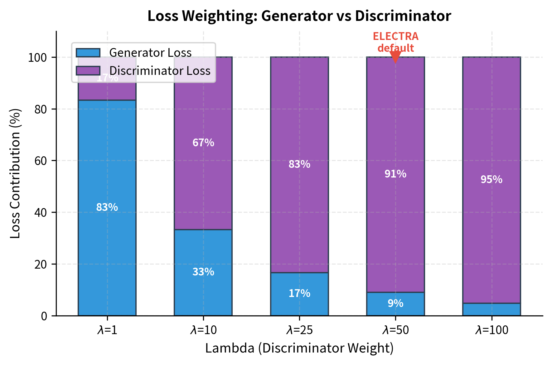
- is a weighting factor that balances the two losses
Why weight the losses differently? The answer lies in what we ultimately care about. After pretraining, we discard the generator and use only the discriminator for downstream tasks. The generator exists solely to create challenging training examples. From this perspective, generator learning is a means to an end: we want it good enough to produce useful replacements, but not so good that it dominates the training budget.
The ELECTRA paper uses , heavily weighting the discriminator loss. This asymmetry reflects the different roles of the two networks. With this weighting, most of the gradient signal flows to the discriminator, which receives the bulk of the learning capacity. The generator still improves through its share of the gradient, producing increasingly plausible replacements that keep the discriminator challenged.
This design creates a beneficial training dynamic. As the generator improves, its replacements become harder to detect. The discriminator must develop more sophisticated representations to keep up. But because the generator is smaller and receives less gradient signal, it cannot outpace the discriminator. The asymmetry maintains a productive difficulty level throughout training.

Why Detection Is Easier Than Generation
The efficiency gain comes from the difference between detection and generation. Predicting the exact token that was masked requires learning fine-grained distinctions in a vocabulary of 30,000+ tokens. Detecting whether a token was replaced requires only a binary decision at each position.
Consider a masked position in the sentence "The [MASK] barked loudly." To predict the correct token, the model must assign probability to "dog" over thousands of alternatives. But to detect a replacement, the model only needs to recognize that "cat" or "piano" in that position feels wrong, even if it cannot pinpoint exactly what should be there.
This asymmetry allows the discriminator to learn useful representations from every position. Original tokens that fit the context well should score high. Replaced tokens, even plausible ones, often have subtle mismatches with surrounding context. The model learns to detect these mismatches, developing representations that capture semantic coherence.
The generator deliberately produces challenging replacements. If it simply inserted random tokens, detection would be trivial. By sampling from a language model, the generator creates replacements that are semantically plausible but contextually imperfect. This forces the discriminator to develop nuanced understanding of context.
Implementing the Generator
The generator is a small transformer that performs MLM. It masks positions, predicts token distributions, and samples replacements.
Let's see the generator in action:
The masking function randomly selects positions to mask. With a 40% masking probability on our 5-token sentence, we typically see 2 positions replaced with [MASK]. The labels tensor stores the original tokens at masked positions for computing the generator loss.
Now let's sample replacements from the generator:
The generator samples tokens for masked positions. Because we're using an untrained generator, the replacements are essentially random from the small vocabulary. With training, the generator would produce more plausible replacements that better challenge the discriminator.
Implementing the Discriminator
The discriminator is a larger transformer that performs binary classification at each position. Its architecture is similar to BERT, but the output layer produces a single logit per position rather than vocabulary logits.
The discriminator has roughly 2-3x more parameters than the generator, matching the ELECTRA design principle. The probabilities show the untrained discriminator's random guesses. With training, these should approach 1.0 for original tokens and 0.0 for replaced tokens, correctly identifying which positions contain generator-produced replacements.
The Complete Training Loop
Training RTD involves three steps per batch: mask inputs, generate replacements, and update both networks.
Let's train on a small corpus to see the dynamics:
Both losses decrease over training. The generator loss drops as it learns to predict masked tokens, while the discriminator loss decreases as it learns to distinguish original from replaced tokens. The initial discriminator loss around 0.69 corresponds to random guessing (binary cross-entropy for 50/50 predictions), confirming the model starts with no knowledge of which tokens are replaced.
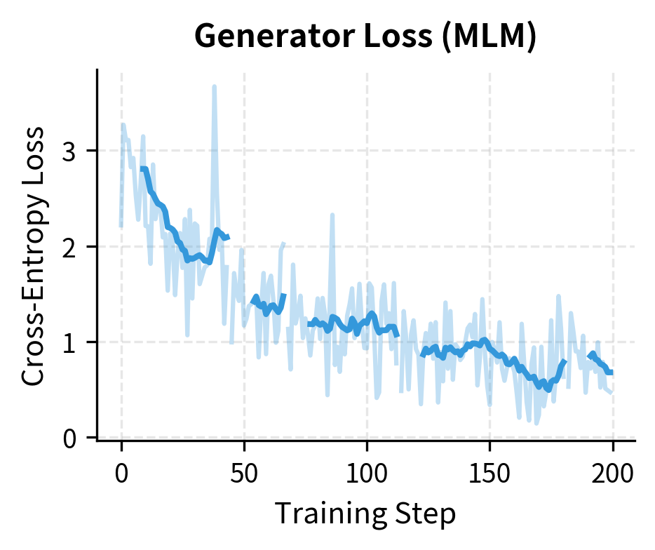
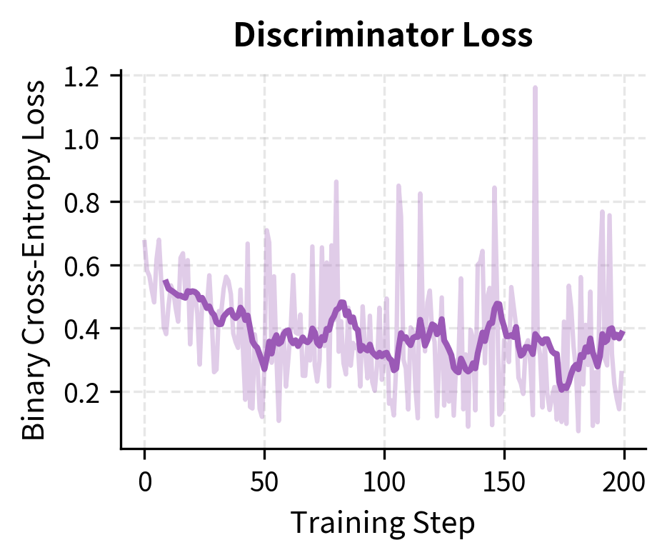
The training dynamics show both losses decreasing. The generator learns to predict masked tokens better, while the discriminator learns to detect replacements. These objectives are complementary: a better generator produces harder replacements, which in turn trains a better discriminator.
RTD Efficiency Advantages
The key advantage of RTD is sample efficiency. Let's quantify the difference:
Weight Sharing and Embedding Tying
The original ELECTRA paper uses weight sharing between generator and discriminator embeddings. This has two benefits: it reduces total parameters and ensures both networks have compatible token representations.
The embedding matrix maps token IDs to dense vectors. Since both networks process the same vocabulary, they can share this large matrix. The generator uses the embeddings directly at its smaller hidden dimension, while the discriminator projects them up to its larger dimension:
The generator embedding dimension determines the shared embedding size. The discriminator projects these embeddings up to its larger hidden dimension. This asymmetry reflects the design principle: the generator needs only enough capacity to produce plausible replacements, while the discriminator needs more capacity to develop rich representations.
Generator Size and Training Dynamics
How big should the generator be relative to the discriminator? Too small, and it produces random, easily-detected replacements. Too large, and it wastes parameters that could go to the discriminator, which is what we actually use for downstream tasks.
The ELECTRA paper found that generator size between 1/4 and 1/2 of the discriminator works best. The sweet spot balances challenging replacements against parameter efficiency.
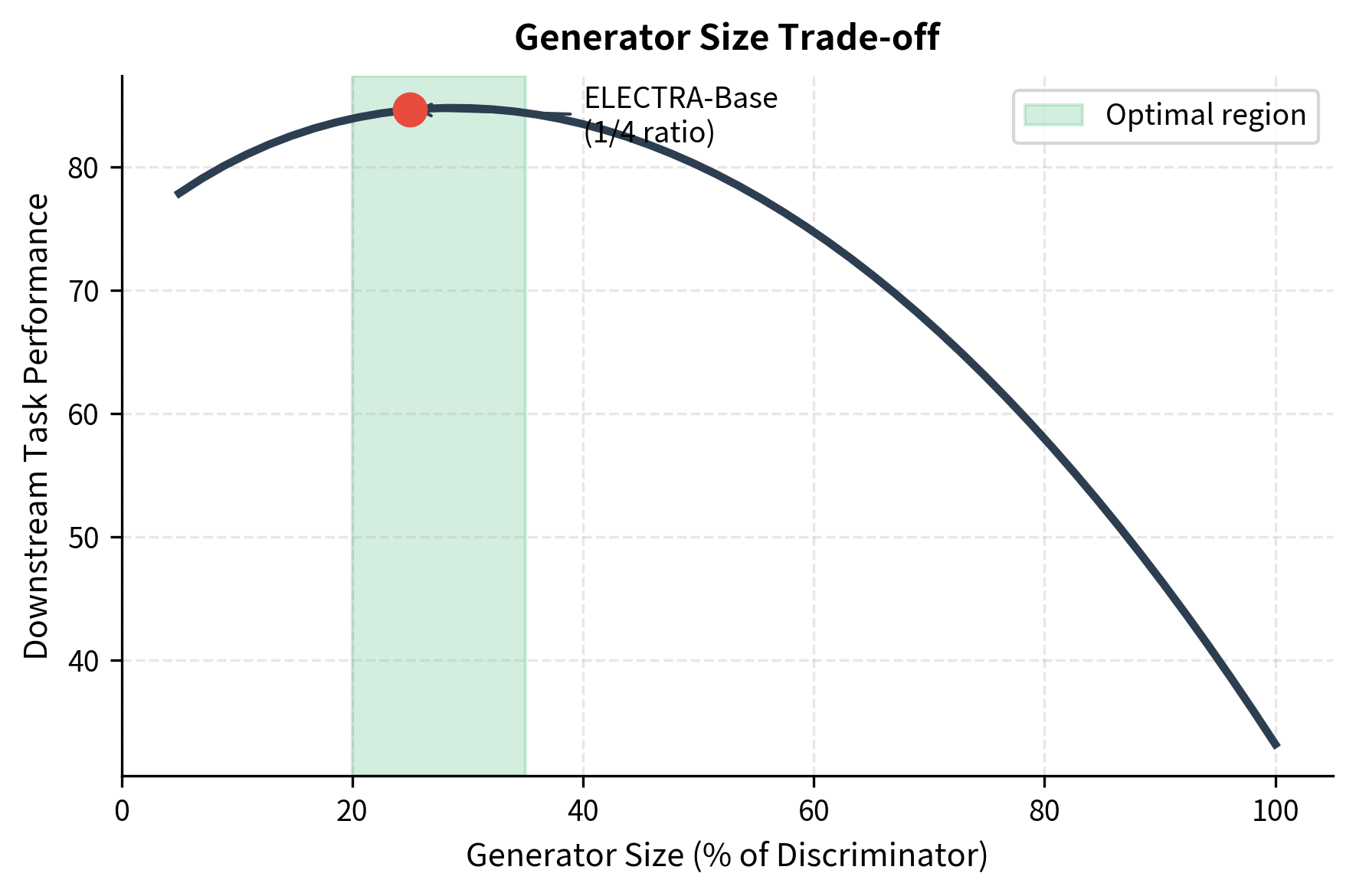
The training dynamics create an interesting interplay. As the generator improves, it produces harder replacements. This forces the discriminator to learn more nuanced representations. But if the generator becomes too good, detection becomes impossible, and learning stalls. The asymmetric sizing naturally prevents this collapse: the smaller generator cannot outpace the larger discriminator.
RTD vs MLM: When to Choose Each
Both objectives produce strong pretrained models, but they have different strengths.
Choose RTD (ELECTRA) when:
- Compute budget is limited.
- You need BERT-level performance with less training.
- Pretraining from scratch rather than using existing checkpoints.
- Sample efficiency matters more than final absolute performance.
Choose MLM (BERT) when:
- You can afford extensive pretraining.
- Using established pretrained checkpoints.
- The ecosystem (fine-tuning code, adapters) assumes MLM architecture.
- Simplicity of single-network training is preferred.
The following table summarizes key differences:
| Aspect | MLM (BERT) | RTD (ELECTRA) |
|---|---|---|
| Loss positions | 15% (masked only) | 100% (all positions) |
| Network count | Single transformer | Generator + discriminator |
| Training efficiency | Baseline | ~4x more efficient |
| Architecture complexity | Simple | Moderate |
| Output head | Vocabulary logits | Binary classifier |
| Downstream model | Full encoder | Discriminator only |
Limitations and Impact
Replaced token detection offers compelling efficiency gains but comes with trade-offs that shape its practical applications.
The two-network training setup adds complexity. Managing separate generator and discriminator networks with different sizes requires careful hyperparameter tuning. The generator learning rate, size ratio, and loss weighting all affect final performance. In contrast, MLM training has fewer moving parts. For practitioners without extensive compute resources to tune these hyperparameters, this complexity can be a barrier.
The discriminator's binary classification objective differs from downstream task objectives. While MLM directly trains vocabulary prediction, which transfers naturally to tasks involving token-level understanding, RTD trains original-vs-replaced classification. The representations transfer well in practice, but the training signal is less directly aligned with common downstream tasks like sequence labeling or question answering.
Weight sharing between generator and discriminator, while parameter-efficient, constrains architecture choices. The generator's embedding dimension becomes the shared base, potentially limiting discriminator capacity. Some practitioners prefer fully separate networks despite the parameter cost.
Despite these limitations, ELECTRA demonstrated that the dominant MLM paradigm was leaving efficiency on the table. The paper's key insight that detection is easier than generation and therefore allows learning from more positions has influenced subsequent work on efficient pretraining. The approach showed that with 1/4 of BERT's compute budget, comparable downstream performance was achievable.
The efficiency gains are most pronounced in the small-to-medium model regime where compute budgets are constrained. At the largest scales, where organizations can afford extensive pretraining, the absolute performance differences between objectives diminish. But for academic researchers, startups, and practitioners training models from scratch, RTD's efficiency remains attractive.
Key Parameters
When implementing RTD training, several parameters affect performance:
-
mask_prob is the fraction of tokens to mask before generating replacements. The default 0.15 (15%) balances training signal against context preservation. Higher rates provide more training examples but degrade generation quality.
-
disc_weight () is the weighting factor for the discriminator loss in the combined objective. ELECTRA uses 50, heavily prioritizing discriminator learning since it's the model used for downstream tasks.
-
generator_size_ratio is the ratio of generator to discriminator model size. Optimal values lie between 0.25 and 0.33. Smaller generators produce easily-detected replacements, while larger generators waste parameters.
-
d_model (discriminator) is the hidden dimension of the discriminator transformer. Larger values increase capacity but require more compute. ELECTRA-Base uses 256, ELECTRA-Large uses 1024.
-
d_model (generator) is the hidden dimension of the generator, typically 1/4 to 1/3 of the discriminator's dimension. This asymmetry ensures the generator produces challenging but not impossible replacements.
-
n_layers (discriminator) is the number of transformer layers in the discriminator. More layers increase representational capacity. ELECTRA-Base uses 12 layers, ELECTRA-Large uses 24.
-
learning_rate can be set separately for generator and discriminator to improve training stability. Typical values range from 1e-4 to 5e-4, with some implementations using slightly lower rates for the generator.
-
temperature controls randomness when sampling from the generator's output distribution. Higher temperatures produce more diverse replacements, while lower temperatures favor the most likely tokens.
Summary
Replaced token detection reformulates pretraining as a detection problem rather than a generation problem. This chapter covered the key concepts:
- Generator-discriminator architecture uses a small network to produce replacement tokens and a larger network to detect them, with only the discriminator used for downstream tasks.
- Detection vs. generation is easier because binary classification requires less capacity than vocabulary prediction, enabling learning from every position.
- Sample efficiency improves by 6-7x because the discriminator loss applies to all positions, not just the 15% that would be masked in MLM.
- Generator sizing at 1/4 to 1/3 of discriminator size balances challenging replacements against parameter efficiency.
- Weight sharing between generator and discriminator embeddings reduces parameters while maintaining compatible representations.
- Training dynamics create complementary learning where better generators produce harder replacements that train better discriminators.
The next chapter explores denoising objectives, a family of pretraining tasks that corrupt inputs in various ways and train models to reconstruct them.
Quiz
Ready to test your understanding? Take this quick quiz to reinforce what you've learned about replaced token detection and ELECTRA's efficient pretraining approach.

Comments