

Deep dive into Qwen's architectural innovations including GQA, SwiGLU activation, and multilingual tokenization. Learn how Qwen optimizes for Chinese and English performance.

This article is part of the free-to-read Language AI Handbook
Choose your expertise level to adjust how many terms are explained. Beginners see more tooltips, experts see fewer to maintain reading flow. Hover over underlined terms for instant definitions.
Qwen Architecture
Introduction
The Qwen (通义千问, Tongyi Qianwen) model family from Alibaba Cloud combines proven architectural innovations with design choices optimized for both Chinese and English performance. First released in August 2023, Qwen models showed that careful attention to tokenization, training data curation, and architectural refinements could produce models rivaling or exceeding Western counterparts, particularly for Asian language tasks.
This chapter examines the architectural decisions, training methodology, and design philosophy that distinguish Qwen from other LLaMA-derived models. We'll explore how Qwen adapts the decoder-only Transformer architecture with specific optimizations for multilingual capabilities, how its training approach balances efficiency with quality, and why these choices matter for applications requiring strong performance across multiple languages.
Chapter roadmap: We'll start by examining Qwen's architectural foundations and how they build upon LLaMA's innovations (Section 2). Then we'll explore the tokenization strategy critical to multilingual performance (Section 3). After understanding the architecture and tokenization, we'll look at training methodology and data composition (Section 4). We'll implement key components to solidify understanding (Section 5), examine the Qwen model family and variants (Section 6), and conclude by discussing limitations and impact (Section 7).
Architecture Overview
Before diving into specific components, let's understand how Qwen fits into the modern LLM landscape and what distinguishes it architecturally.
Foundation: Decoder-Only Transformer
Qwen adopts the decoder-only Transformer architecture, following the successful pattern established by GPT and refined by LLaMA. Like its predecessors, Qwen uses:
- Causal (left-to-right) attention masking for autoregressive generation
- Single unified architecture for all tasks
- Input and output sharing the same embedding space
Key Architectural Differences
Qwen combines proven innovations from LLaMA with additional refinements:
| Component | LLaMA | Qwen | Rationale |
|---|---|---|---|
| Normalization | RMSNorm (pre-norm) | RMSNorm (pre-norm) | Training stability |
| Activation | SwiGLU | SwiGLU | Model quality |
| Positional Encoding | RoPE | RoPE | Length extrapolation |
| Attention | Multi-head (7B) / GQA (70B) | GQA (all sizes) | Memory efficiency |
| Attention Bias | No bias | QKV bias | Improved attention quality |
| Vocabulary Size | 32,000 | 151,936 | Multilingual optimization |
| Embedding Tying | Tied | Untied | Better output distribution |
The most notable differences are the addition of bias terms in attention projections, the much larger vocabulary optimized for Chinese, and the use of Grouped-Query Attention across all model sizes.
Core Architectural Components
This section builds your understanding of Qwen's key innovations step by step. We'll start with the attention mechanism, where Qwen makes its most impactful efficiency choice, then explore the feed-forward network and positional encoding. For each component, we'll first build intuition about the problem being solved, then examine the mathematical formulation, and finally see it in code.
Grouped-Query Attention
To understand why Qwen uses Grouped-Query Attention (GQA), we first need to understand the memory bottleneck in transformer inference.
The problem: KV cache explosion
During autoregressive generation, transformers must store the key (K) and value (V) vectors for all previously generated tokens. This "KV cache" allows the model to attend to its full history without recomputing everything at each step. For a model with layers, attention heads, head dimension , and sequence length , the cache requires:
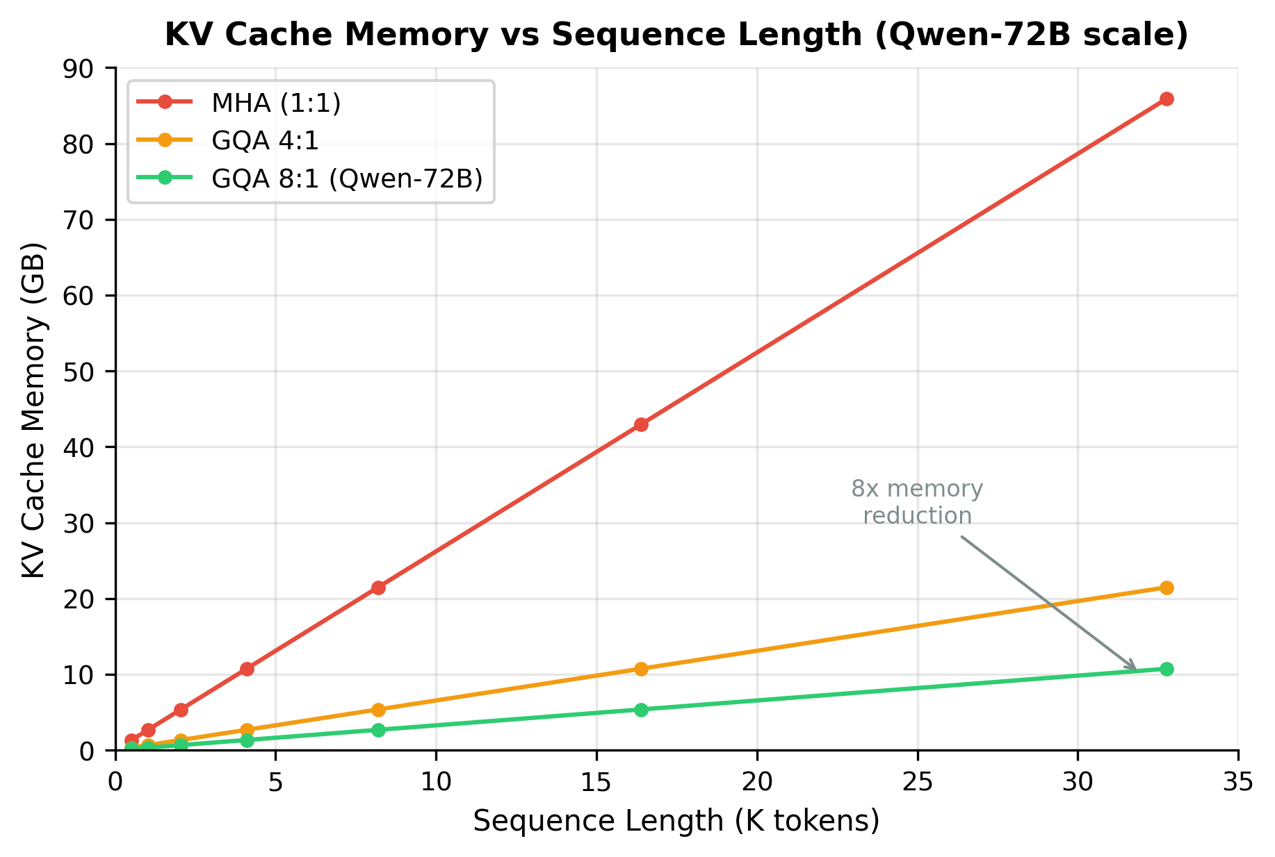
For Qwen-72B generating a 4096-token sequence in FP16, this exceeds 40GB just for the cache. The insight behind GQA is that not every query head needs its own unique key-value representation, so we can share KV heads across groups of query heads to dramatically reduce this memory burden.
The solution: sharing key-value heads
While LLaMA-7B uses standard multi-head attention (MHA), Qwen employs Grouped-Query Attention (GQA) across all model sizes. GQA strikes a balance between the quality of MHA and the efficiency of Multi-Query Attention (MQA).
In standard multi-head attention, each query head has its own dedicated key and value heads. GQA groups multiple query heads together to share a single set of key-value heads. This reduces memory requirements while preserving most of the representational capacity.
Understanding the attention variants
Before diving into the formulas, let's build intuition about the three attention variants:
-
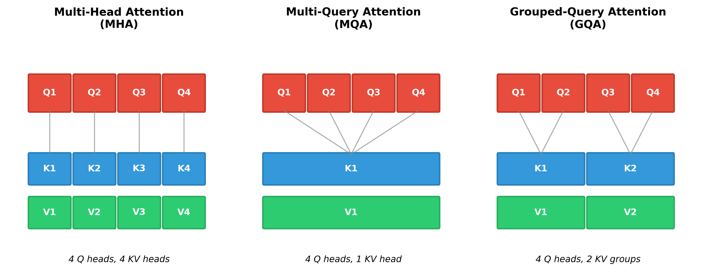
Multi-Head Attention (MHA): The original design. Each query head gets its own private key-value pair. Maximum expressiveness, but maximum memory cost. Think of it as giving each employee their own filing cabinet.
-
Multi-Query Attention (MQA): The extreme efficiency approach. All query heads share a single key-value pair. Minimal memory, but information gets compressed. Like having everyone share one filing cabinet.
-
Grouped-Query Attention (GQA): The balanced solution. Small groups of query heads share key-value pairs. Qwen uses this because it retains most of MHA's quality while achieving most of MQA's efficiency gains.
The mathematical formulation
Now we can understand the formal definition. The overall GQA computation concatenates the outputs from all attention heads and projects them back to the model dimension:
where:
- : the query, key, and value tensors derived from the input hidden states
- : the output of the -th attention head, capturing what information token should attend to
- : the total number of query heads (e.g., 32 for Qwen-7B, 64 for Qwen-72B)
- : the output projection matrix of shape that recombines head outputs
- : concatenation along the head dimension, stacking all head outputs together
Each individual head computes attention using its query projection but shares key-value projections with other heads in its group. This is where the efficiency gain comes from:
where:
- : the query input for head (unique to each head)
- : the query projection matrix for head (unique to each head)
- : a grouping function that maps query head to its corresponding KV group index
- : the key and value inputs for the group containing head (shared within group)
- : the shared key and value projection matrices for that group
How grouping works in practice
The grouping function determines which query heads share KV heads. For a model with query heads and key-value heads:
Let's trace through two concrete examples:
-
Qwen-7B: 32 query heads, 32 KV heads (ratio 1:1). Here , so each query head has its own KV head. This is equivalent to standard MHA, the safe choice for a smaller model.
-
Qwen-72B: 64 query heads, 8 KV heads (ratio 8:1). Every 8 consecutive query heads share the same KV head. Query heads 0-7 share KV head 0, heads 8-15 share KV head 1, and so on. This provides an 8× reduction in KV cache memory.
Why this works
The intuition for why grouping works is that different query heads often look for similar patterns in the keys and values. By forcing them to share, we impose a useful regularization. Empirically, researchers found that models with GQA ratios up to 8:1 show minimal quality degradation while achieving substantial memory and speed improvements.
Summary of advantages
- Reduced KV cache memory: Fewer KV heads means smaller cache during generation (8× reduction for Qwen-72B)
- Faster inference: Less memory bandwidth needed to load KV cache, directly improving tokens/second
- Maintained quality: Grouping preserves most of MHA's representational capacity through shared but still diverse key-value representations
Attention with Bias
Having understood how Qwen organizes its attention heads, we now turn to a subtler design choice: whether to include bias terms in the attention projections.
The design question
When projecting hidden states to queries, keys, and values, we have a choice:
LLaMA follows the trend of removing all bias terms, arguing that the weight matrices alone have sufficient capacity and that removing bias simplifies the model. Qwen takes the opposite stance, adding bias to the Query, Key, and Value projections.
Why bias might help
The intuition is subtle but important. Bias terms provide a learned "default" activation that doesn't depend on the input. In attention, this means:
- Queries can have a baseline direction they search in, independent of the current token
- Keys can have a baseline "signature" that makes certain patterns more or less likely to match
- Values can contribute baseline information even before considering specific content
Think of it like this: without bias, attention patterns must emerge entirely from token-token interactions. With bias, the model can learn that "queries from this head should generally attend more to earlier positions" or "values should include this baseline information regardless of content."
The parameter cost
This flexibility comes at minimal cost. For Qwen-7B:
Compared to the total attention parameters per layer (~67M), this is about 0.02%. Qwen's researchers found this negligible overhead provides measurable quality improvements, particularly in tasks requiring nuanced attention patterns.
Implementation
Unlike LLaMA which removes all bias terms from linear projections, Qwen adds bias to the Query, Key, and Value projections:
The output shape matches the input shape, confirming the attention module correctly processes the sequence while preserving dimensions. The bias parameters add only 0.02% overhead to the attention layer, but Qwen's researchers found this small addition improves attention pattern learning. The 128-dimensional heads (4096 / 32) provide sufficient capacity for complex attention patterns. While LLaMA removes biases for simplicity and to reduce parameters, Qwen found that the small parameter increase (less than 0.1% of total) provides meaningful quality improvements.
SwiGLU Feed-Forward Network
After attention aggregates information across positions, the feed-forward network (FFN) processes each position independently, adding nonlinearity and increasing the model's representational capacity. Here we explore why Qwen chose SwiGLU over simpler alternatives.
The evolution of feed-forward design
The original Transformer used a simple two-layer FFN with ReLU activation:
This works, but researchers discovered that gated variants perform better. The key insight: instead of applying a single nonlinearity, use one transformation to decide what information to pass through (the gate) and another to decide which information is available (the values).
The gating mechanism
SwiGLU introduces element-wise multiplication between two parallel branches:
Let's unpack each part:
-
Gate branch (): Projects the input to an intermediate dimension, then applies Swish activation. The Swish output ranges from near-zero (suppress) to unbounded positive (amplify).
-
Value branch (): Projects the input to the same intermediate dimension. These are the "candidate" values that might pass through.
-
Element-wise product (): For each element, the gate controls how much of the corresponding value passes through. Near-zero gate means that value is suppressed; large positive gate means that value is amplified.
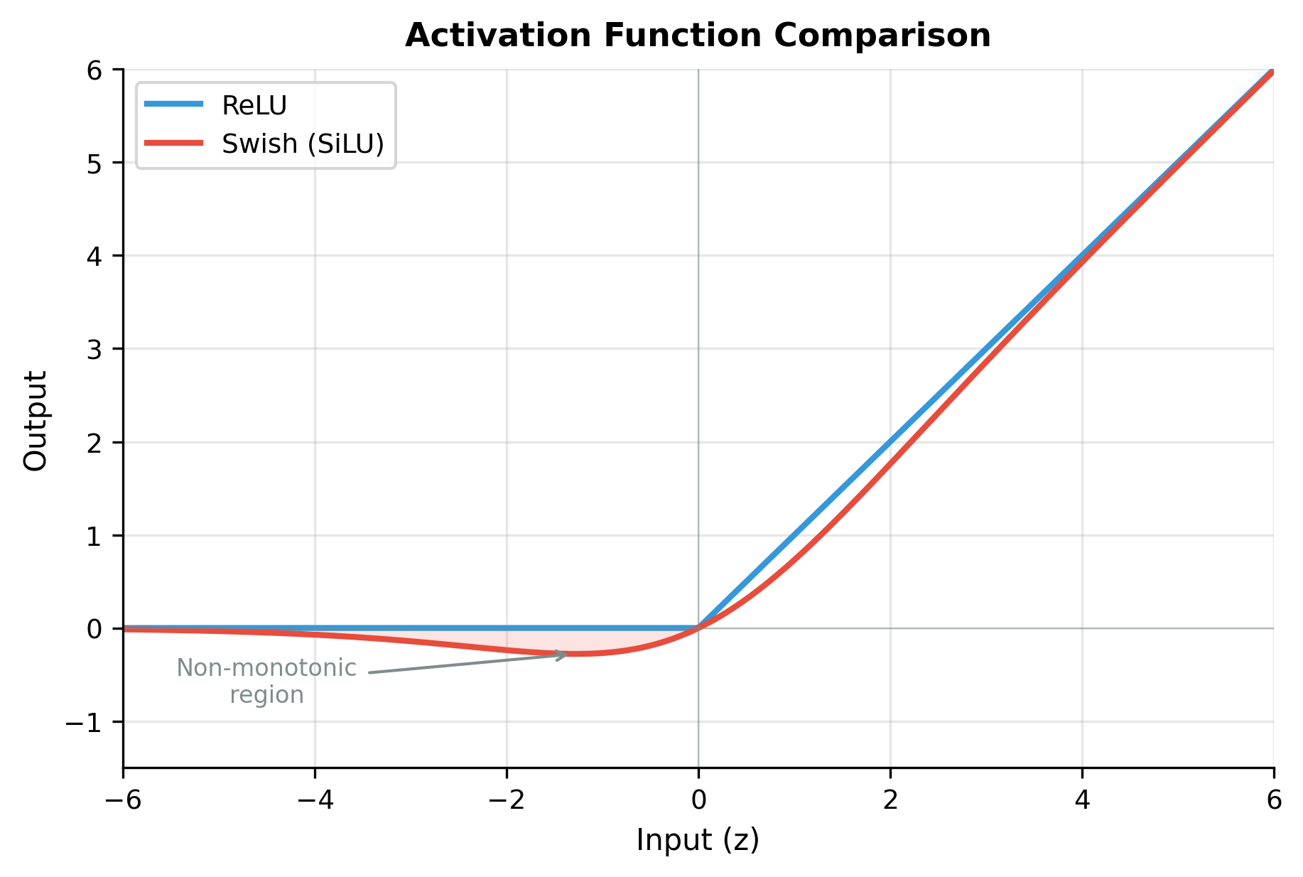
The Swish activation
Why Swish rather than ReLU for the gate? Swish provides smooth, non-monotonic gating:
Key properties that make Swish effective:
- Smooth gradients: Unlike ReLU's hard cutoff at zero, Swish transitions gradually, improving gradient flow during training
- Non-monotonic: For small negative inputs, Swish actually outputs small negative values before approaching zero. This allows the gate to preserve subtle negative signals
- Self-gating: The term acts as a soft switch on the term itself
The complete MLP
After the gated transformation, we project back to the model dimension:
where has shape . The intermediate dimension is typically rather than the standard . This adjustment accounts for SwiGLU having three projection matrices instead of two, keeping the total parameter count similar to a standard FFN.
Implementation
Like LLaMA, Qwen uses the SwiGLU activation function in its feed-forward layers:
Analyzing the output
The MLP parameters dominate each transformer layer, accounting for roughly two-thirds of per-layer parameters. The 2.69x expansion ratio (rather than the standard 4x) compensates for SwiGLU's three projections instead of two, keeping total parameter count comparable to standard FFN layers while providing the gating mechanism's quality benefits.
Why gating matters
The key insight is that not all intermediate features are equally useful for every input. In a standard FFN, every intermediate neuron contributes to every output (modulated only by ReLU killing negative values). With SwiGLU, the gate branch learns when each intermediate feature should contribute, creating input-dependent computation paths. This is a form of learned sparsity that improves model quality without increasing inference cost.
RoPE: Rotary Positional Embeddings
Transformers process sequences in parallel, treating each position identically. This is computationally efficient but creates a problem: how does the model know that token 5 comes before token 10? The answer lies in positional encoding, and Qwen uses Rotary Position Embeddings (RoPE), the same approach as LLaMA.
The positional encoding challenge
Early transformers used absolute positional embeddings: learn a vector for position 0, another for position 1, and so on. This has two problems:
- Length limitation: The model can only handle positions it saw during training
- No relative reasoning: Positions 10-15 look completely different from positions 100-105, even though the relationship (5 tokens apart) is identical
What we really want is a way to encode position such that attention scores depend on relative distance between tokens, not their absolute positions.
The rotation insight
RoPE achieves this by encoding position as a rotation in embedding space. The key insight is that when two rotations are composed, the result depends only on their angular difference:
If we rotate queries by their position and keys by their position, then when we compute attention (which involves a dot product between queries and keys), the rotation effect depends only on the relative distance.
How rotation encodes position
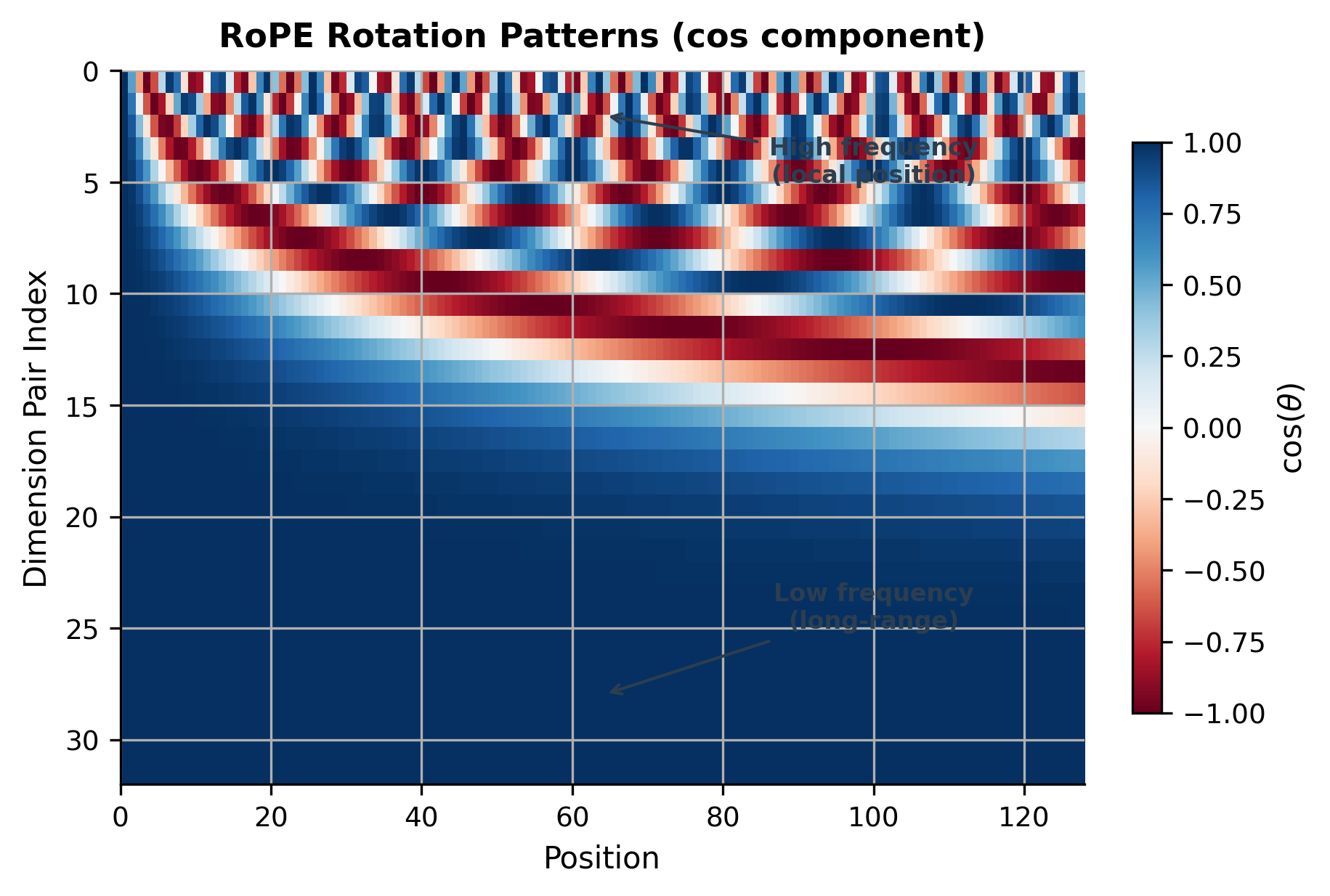
For each position , we construct a rotation matrix that rotates pairs of dimensions in the embedding space. The rotation angle depends on both the position and the dimension pair:
where indexes the dimension pair (there are pairs for dimension ) and is the position. Lower-frequency rotations (larger ) encode longer-range position information; higher-frequency rotations (smaller ) encode fine-grained local position.
The relative position property
The key property emerges when we compute attention scores. Given a query at position and a key at position :
The attention score depends only on , the rotation corresponding to the relative distance . This means:
- Tokens 5 positions apart always have the same relative encoding, regardless of absolute position
- The model can potentially generalize to longer sequences than it was trained on
- Nearby tokens have similar rotations; distant tokens have dissimilar rotations
Implementation
Qwen uses the same RoPE implementation as LLaMA for positional encoding, which encodes position through rotation of query and key vectors:
Understanding the code
The implementation uses complex number arithmetic as an efficient way to apply 2D rotations. The precompute_freqs_cis function generates the rotation angles for each position and dimension pair, stored as complex numbers (cosine + i·sine). The apply_rotary_emb function then applies these rotations by treating pairs of real dimensions as complex numbers and multiplying.
This approach is mathematically equivalent to applying rotation matrices but is much more efficient on modern hardware. The key insight remains: after rotation, attention scores between queries and keys naturally encode relative position, enabling the model to reason about token relationships regardless of their absolute positions in the sequence.
Tokenization Strategy
One of Qwen's most distinctive features is its tokenization approach, optimized for multilingual text with particular emphasis on Chinese.
Large Multilingual Vocabulary
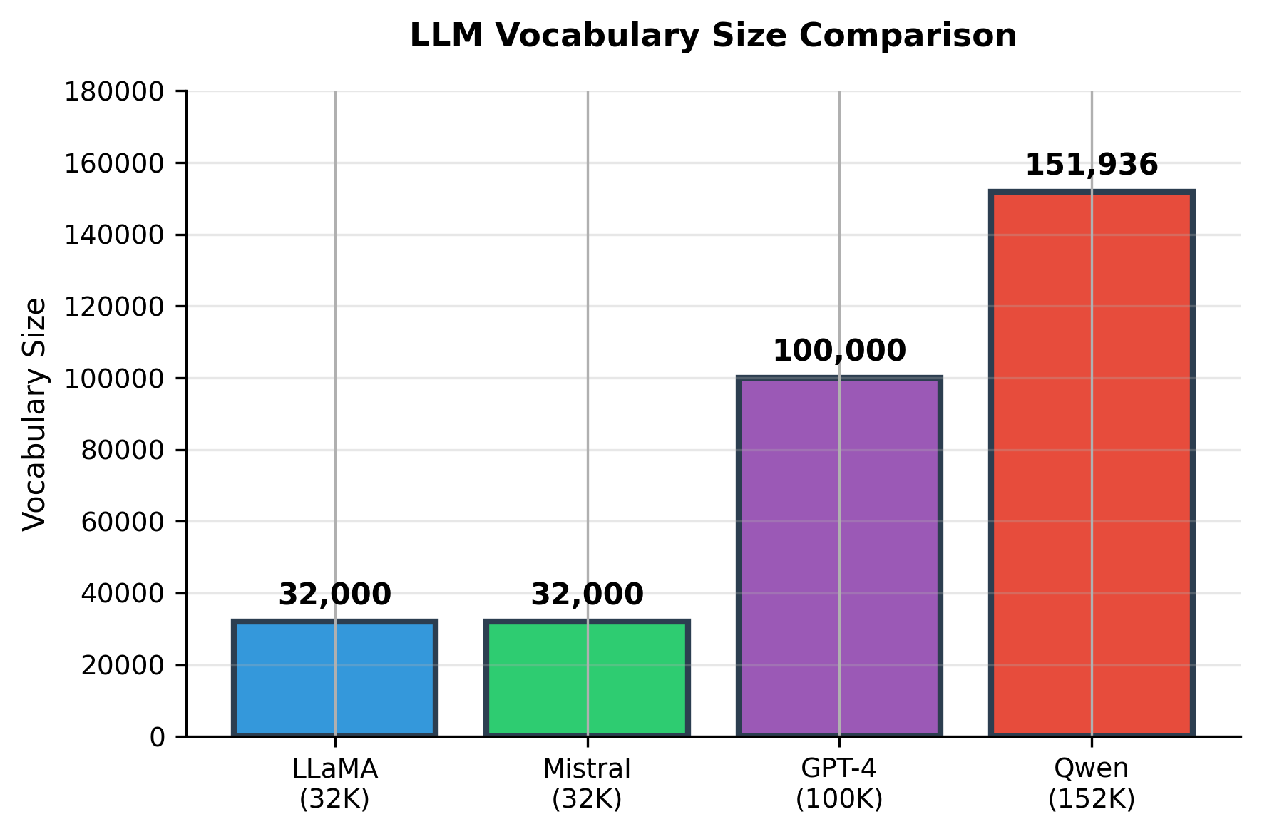
Qwen uses a vocabulary of 151,936 tokens, nearly 5× larger than LLaMA's 32,000. This design decision has important implications:
Advantages of larger vocabulary:
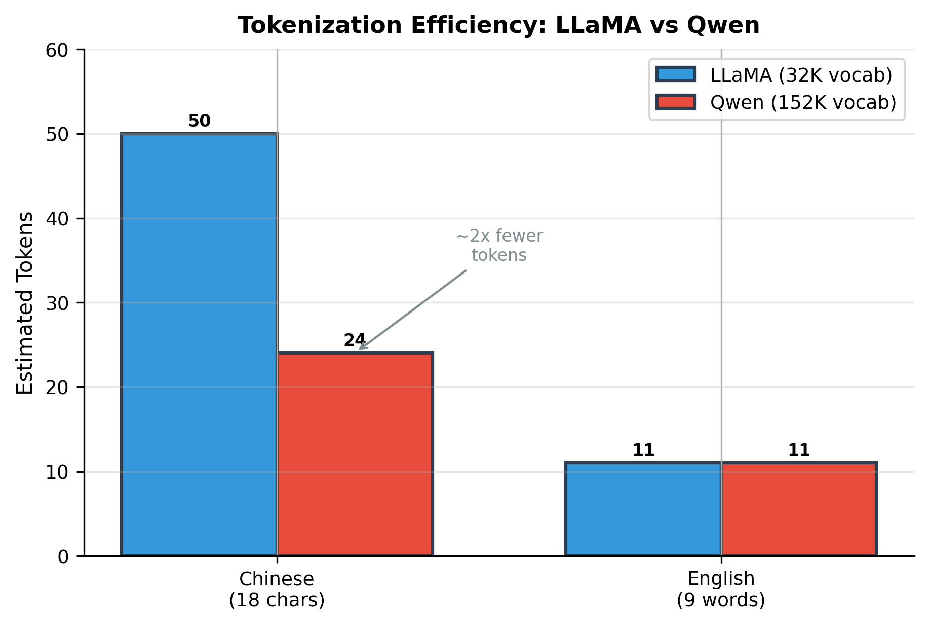
- Better Chinese representation: Many Chinese characters receive their own tokens rather than being split into byte-level pieces
- Fewer tokens per text: Chinese text requires significantly fewer tokens, improving both efficiency and context utilization
- Improved multilingual coverage: Better handling of Korean, Japanese, and other Asian languages
Trade-offs:
- Larger embedding matrices: Increases model size by approximately 0.5B parameters for Qwen-7B
- Sparser token distributions: Each token appears less frequently during training
- Memory overhead: Larger vocabulary requires more memory for softmax computation
Byte-Level BPE with Special Handling
Qwen uses Byte-Pair Encoding (BPE) at the byte level, similar to GPT-4, but with additional handling for CJK (Chinese, Japanese, Korean) characters:
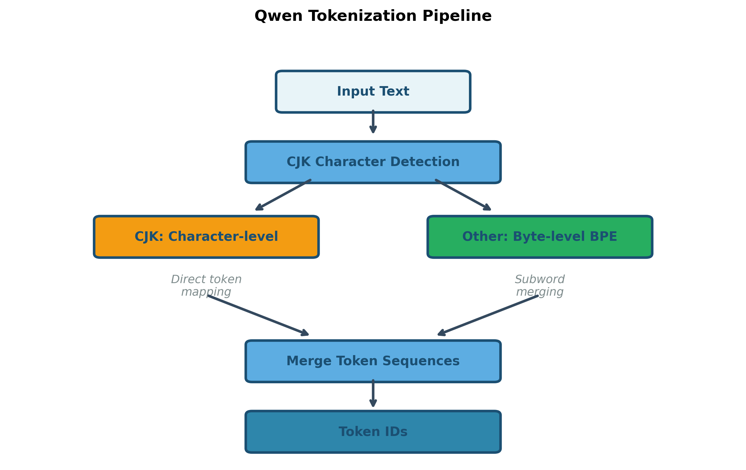
The tokenization strategy ensures:
- No unknown tokens: Byte-level fallback handles any input
- Efficient CJK: Common characters get dedicated tokens
- Balanced encoding: Similar information density across languages
Training Methodology
Training Data Composition
Qwen is trained on approximately 3 trillion tokens, significantly more than LLaMA's 1-1.4 trillion:
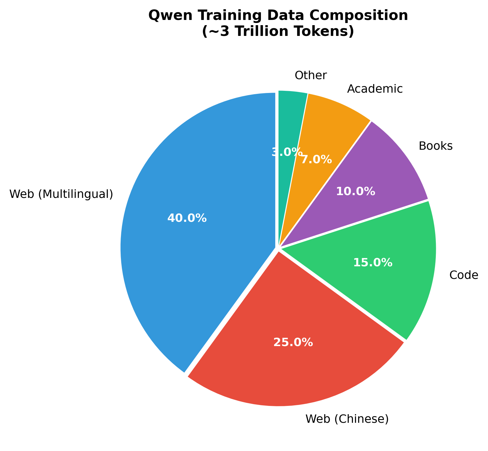
Key data characteristics:
- Multilingual balance: Substantial Chinese content alongside English and other languages
- Code inclusion: Programming languages for coding capabilities
- Quality filtering: Extensive deduplication and quality scoring
- Domain diversity: Academic papers, books, web text, and specialized corpora
Training Configuration
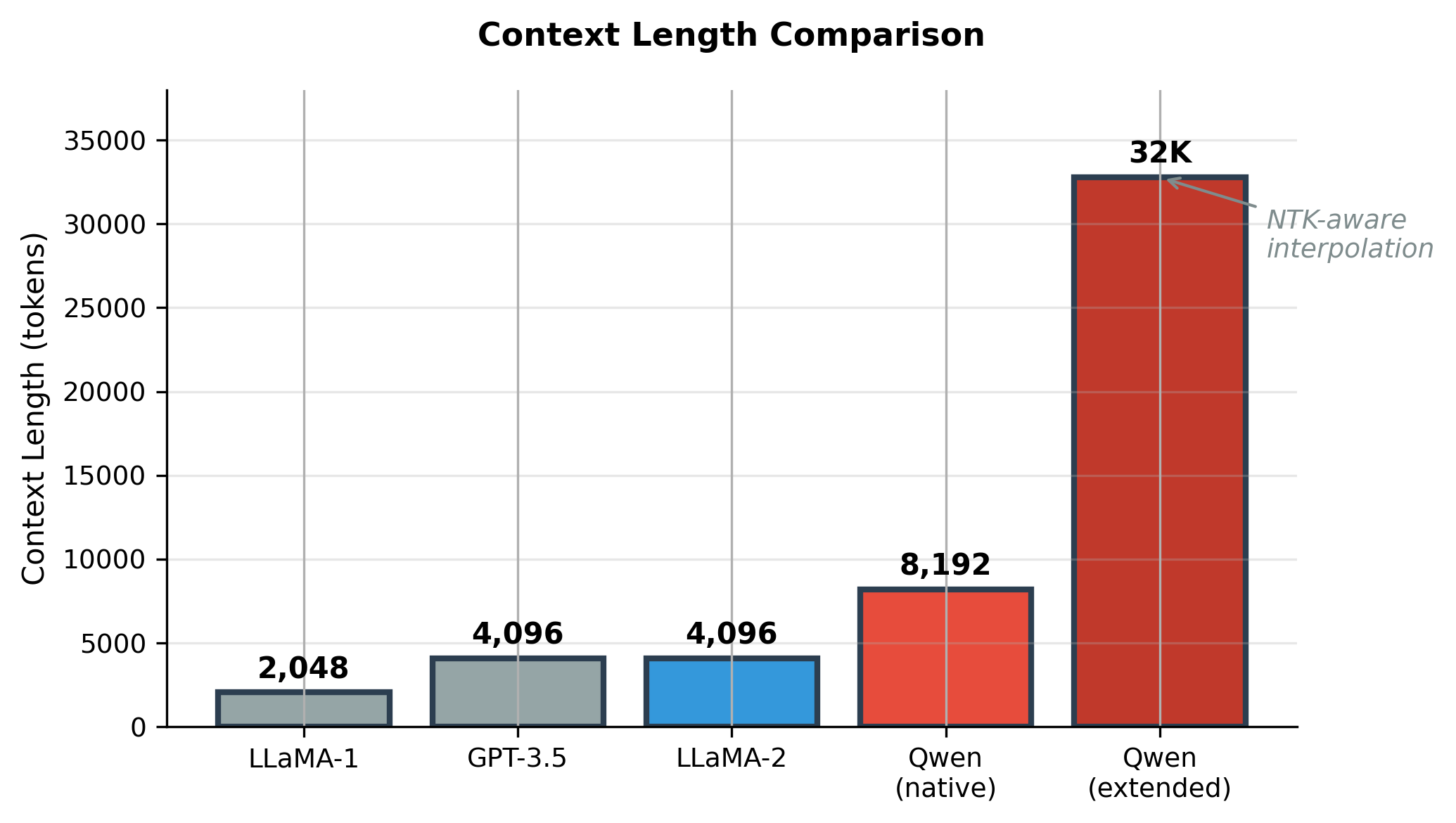
Qwen's training follows similar principles to LLaMA but with extended context length (8192 vs 2048) and more training tokens. The longer context is enabled through careful RoPE scaling and NTK-aware interpolation.
Context Length Extension
Qwen supports 8192 token context through training, with the ability to extend further using position interpolation techniques:
Complete Model Implementation
Having explored each component individually, we now assemble them into a complete Qwen model. This integration reveals how the pieces fit together and provides a reference implementation you can extend for your own experiments.
The journey from components to complete model follows this path:
- Configuration: Define the hyperparameters that determine model size and behavior
- Normalization: Implement RMSNorm, which stabilizes training by normalizing hidden states
- Transformer block: Combine attention, FFN, and normalization into the repeating unit
- Full model: Stack blocks with embeddings and output projection
Model Configuration
We start by defining a configuration class that captures all the hyperparameters. This makes it easy to instantiate different model sizes and ensures consistency across components:
The configuration reveals several key design decisions. Note how GQA ratio varies: Qwen-7B uses 1:1 (equivalent to MHA), while Qwen-72B uses 8:1 for significant memory savings. The intermediate size follows the ~2.7x rule we discussed for SwiGLU. The large vocabulary (151,936) is constant across all sizes, optimized for Chinese characters.
RMSNorm Implementation
Before assembling the transformer block, we need our normalization layer. RMSNorm (Root Mean Square Layer Normalization) is simpler than the original LayerNorm: it normalizes by the root mean square of activations without centering (subtracting the mean).
RMSNorm normalizes input magnitudes while preserving the mean, unlike LayerNorm which centers around zero. The output standard deviation is close to 1.0, indicating proper normalization. With only 4,096 learnable parameters (the scale weights), RMSNorm adds minimal overhead while providing training stability.
The mathematical formulation is:
where is the hidden dimension, is a small constant for numerical stability, and is the learnable scale parameter. By skipping the mean centering of LayerNorm, RMSNorm is slightly faster while empirically performing just as well.
Complete Transformer Block
Now we combine attention, FFN, and normalization into a single transformer block. This is the fundamental repeating unit of the model. Qwen-7B stacks 32 of these blocks.
The block follows the pre-norm architecture pattern, where normalization happens before each sub-layer rather than after. This improves training stability, especially for deep networks:
The parameter distribution shows MLP dominates at roughly 65% of layer parameters, with attention at about 35%. This is typical for modern transformers using SwiGLU. The normalization layers contribute negligibly to parameter count but are critical for training stability.
The code reveals the pre-norm pattern in action: each sub-layer computes residual = hidden_states before normalization, then adds the sub-layer output back (hidden_states = residual + hidden_states). This residual connection is essential. It provides a direct gradient pathway during backpropagation and allows each layer to learn a refinement of its input rather than a complete transformation.
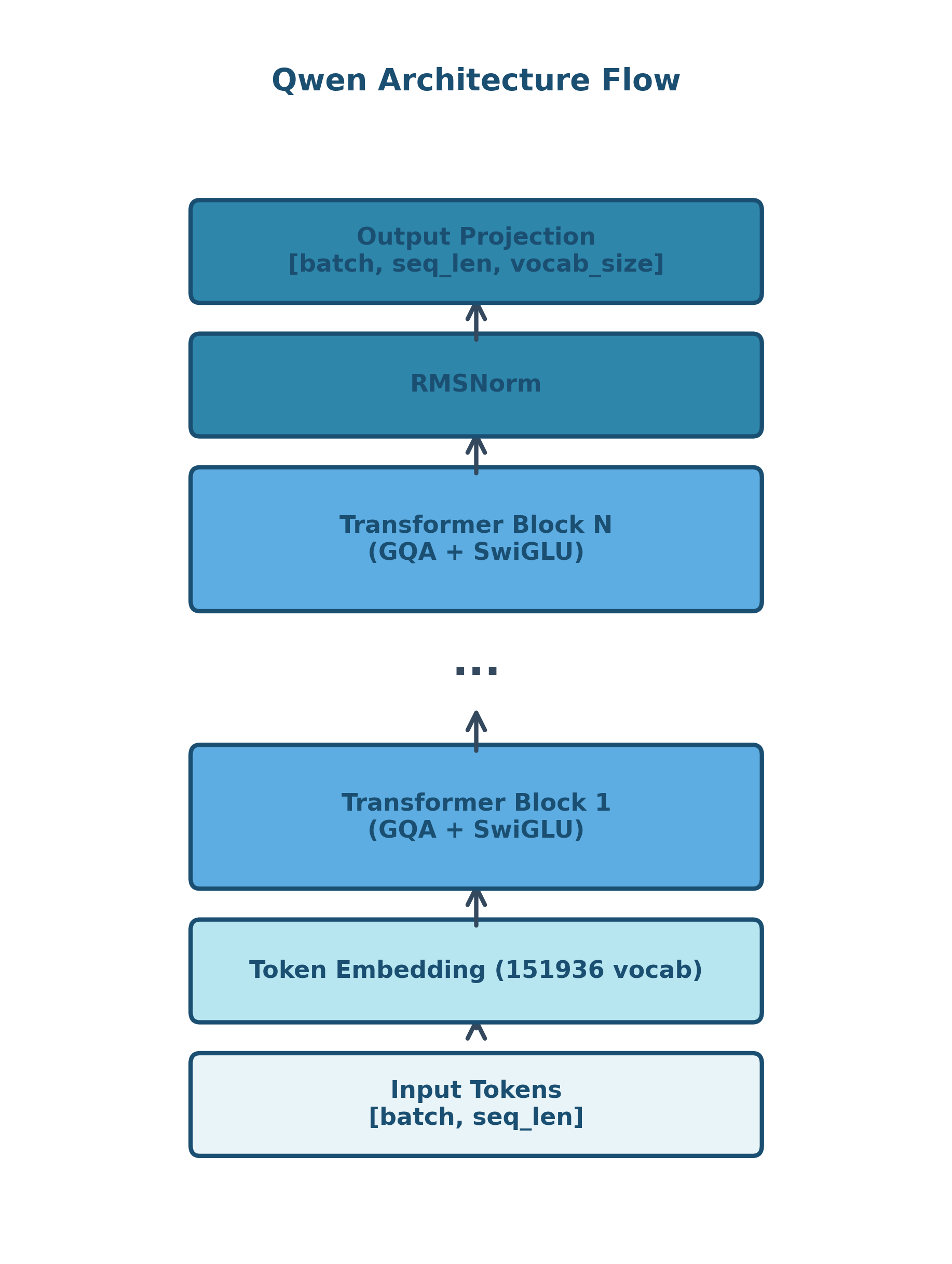
Complete Qwen Model
Finally, we assemble the complete model by wrapping our transformer blocks with:
- Token embeddings: Convert token IDs to dense vectors
- Stacked transformer blocks: The core computation
- Final normalization: Stabilize the output before prediction
- Language model head: Project back to vocabulary size for next-token prediction
The model successfully processes input tokens through all layers and produces vocabulary logits. With untied embeddings, both the input embedding and output LM head have separate parameters, each accounting for a significant fraction of total model size. This is particularly pronounced in Qwen due to its large vocabulary.
A note on tied vs. untied embeddings
Some models (like the original GPT-2) tie the input embedding and output projection, using the same weight matrix for both. This saves parameters but forces the embedding space to serve double duty: representing input tokens and producing output logits. Qwen untied these, allowing the input embedding to specialize for contextual representation and the output head to specialize for prediction. The cost is doubling the embedding parameters (about 0.6B for Qwen-7B), but the quality gain justifies this for large models.
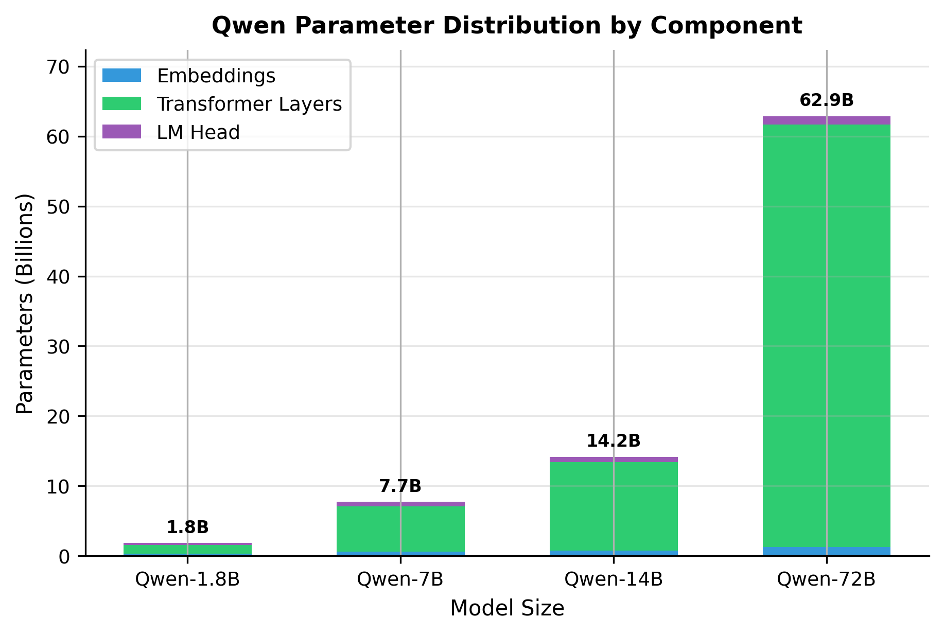
Parameter Count Analysis
Understanding where parameters live helps with capacity planning and debugging. Let's systematically count parameters for each Qwen variant:
Notice how the large vocabulary (151,936 tokens) significantly impacts the embedding and LM head parameters. For Qwen-7B, embeddings alone account for approximately 0.6B parameters (about 8% of total), compared to less than 3% in LLaMA-7B.
Model Variants and Family
Qwen Model Family
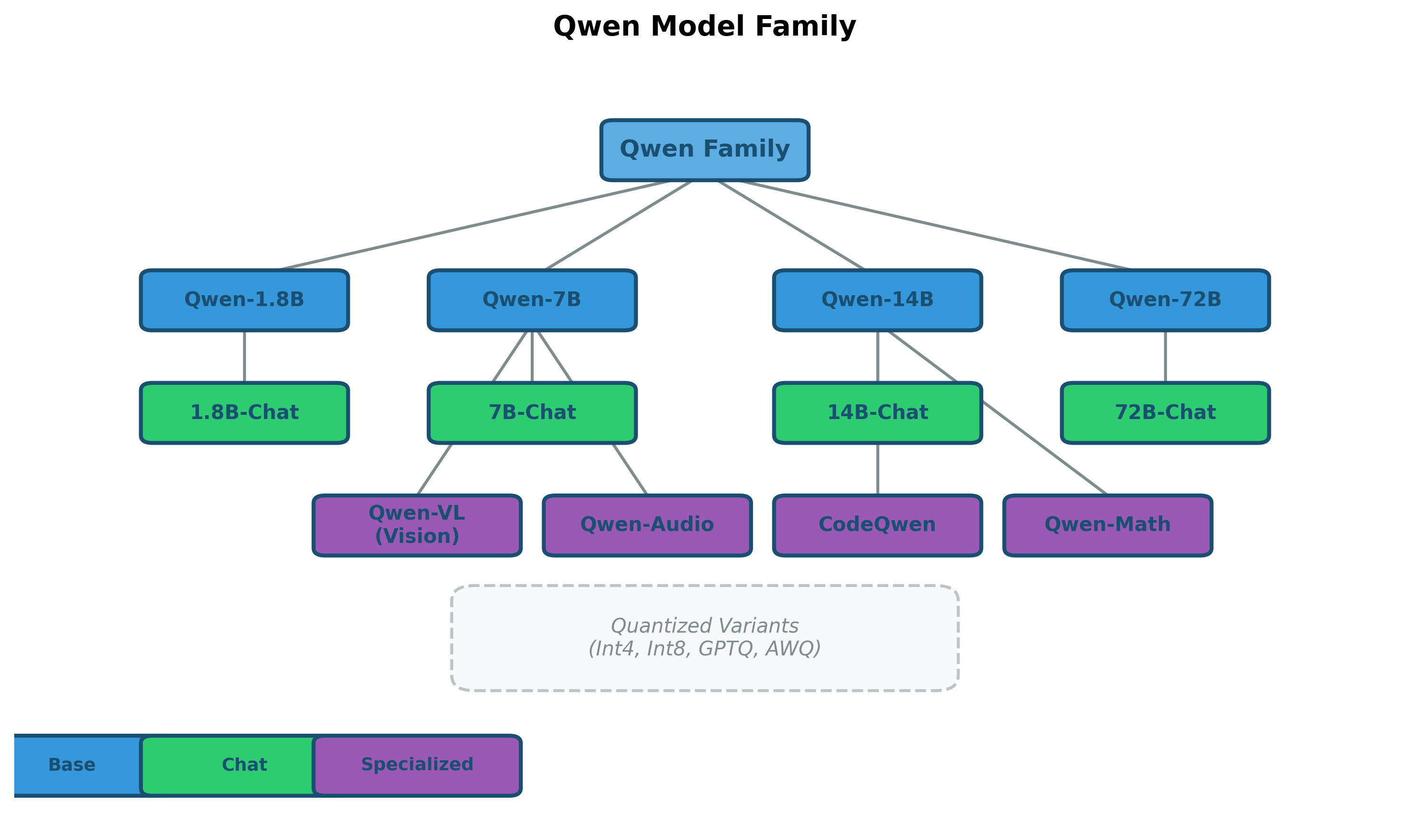
The Qwen family has expanded significantly since its initial release:
Base models (various sizes):
- Qwen-1.8B, Qwen-7B, Qwen-14B, Qwen-72B
- Pre-trained on diverse multilingual data
- Strong foundation for fine-tuning
Chat variants:
- Instruction-tuned using SFT and RLHF
- Optimized for conversational use cases
- Safety-aligned for deployment
Specialized variants:
- Qwen-VL: Vision-language model for image understanding
- Qwen-Audio: Audio understanding and generation
- CodeQwen: Specialized for code generation and understanding
- Qwen-Math: Enhanced mathematical reasoning
Qwen 2 Improvements
Qwen 2, released in 2024, introduced several architectural refinements:
Limitations and Impact
Current Limitations
Despite its strengths, Qwen has several notable limitations that affect its practical use:
Technical constraints:
- Large vocabulary increases memory requirements
- Untied embeddings add parameters without proportional quality gains in all tasks
- Slower tokenization due to larger vocabulary lookup
Capability gaps:
- Hallucination remains an issue, particularly for factual queries
- Long-context performance degrades beyond training length despite RoPE
- Mathematical reasoning, while improved, still trails specialized models
Deployment considerations:
- 72B model requires significant infrastructure
- Quantization needed for consumer hardware deployment
- Inference speed impacted by large vocabulary softmax
These limitations are being actively addressed in subsequent Qwen versions, with Qwen 2 showing particular improvements in efficiency and capability gaps.
Impact on the Field
Qwen's contributions extend beyond its technical specifications:
Demonstrating multilingual competence:
- Proved that non-English-first models can achieve competitive performance
- Showed the importance of vocabulary design for multilingual capability
- Influenced tokenization strategies in subsequent models
Open-source ecosystem:
- Released weights under permissive licenses (Apache 2.0 for many variants)
- Provided strong baseline for Chinese NLP research
- Enabled fine-tuning for specialized Chinese/multilingual applications
Architectural validation:
- Confirmed benefits of GQA across model sizes
- Validated attention bias addition for quality improvement
- Demonstrated viability of larger vocabularies with proper training
The success of Qwen models has encouraged other organizations to invest in multilingual model development and has highlighted the importance of considering non-English languages in LLM design from the ground up.
Key Architecture Parameters
When working with or adapting Qwen models, these parameters have the most significant impact:
Model Dimension Parameters:
hidden_size: The model's hidden dimension (2048 for 1.8B, up to 8192 for 72B). Determines representation capacity and scales quadratically with attention compute.num_hidden_layers: Number of transformer blocks (24-80 across sizes). More layers enable deeper reasoning but increase inference latency linearly.intermediate_size: FFN hidden dimension, typically ~2.7xhidden_size. Controls MLP capacity, which dominates parameter count.
Attention Parameters:
num_attention_heads: Query head count (16-64 across sizes). More heads enable diverse attention patterns but increase memory for attention scores.num_kv_heads: Key-value head count for GQA. Lower ratios (e.g., 8:1 in Qwen-72B) significantly reduce KV cache memory during generation.use_qkv_bias: Whether to include bias in attention projections (True for Qwen). Small parameter overhead for quality gains.
Sequence Parameters:
max_position_embeddings: Maximum context length (8192 native, extendable to 32K+). Affects RoPE frequency computation and KV cache size.rope_theta: Base frequency for RoPE (10000.0 default). Higher values enable better length extrapolation.
rms_norm_eps: Epsilon for numerical stability in RMSNorm (1e-6). Rarely needs adjustment but critical for mixed-precision training.
Vocabulary:
vocab_size: Token vocabulary size (151,936 for Qwen). Larger vocabularies improve multilingual efficiency but increase embedding/LM head parameters significantly.
Summary
Qwen adapts LLaMA's foundation for multilingual, particularly Chinese-focused, applications. By combining proven innovations (RMSNorm, SwiGLU, RoPE) with targeted modifications (large vocabulary, attention bias, GQA across all sizes), Qwen achieves strong performance across both Chinese and English tasks.
Key takeaways:
-
Vocabulary design matters for multilingual models: Qwen's 151,936 token vocabulary, while adding parameters, enables 2x more efficient tokenization of Chinese text. This directly translates to better context utilization and reduced inference cost for Chinese applications.
-
Architectural refinements compound: Adding bias to attention projections and using GQA universally are small changes individually, but together they improve both quality and efficiency. The lesson: don't dismiss seemingly minor architectural modifications.
-
Training data composition shapes capability: Qwen's strong Chinese performance stems from deliberate training data curation, not just architectural choices. Balanced multilingual training from the start produces better results than post-hoc adaptation.
-
Open weights accelerate progress: By releasing model weights openly, Alibaba enabled rapid ecosystem development. The proliferation of Qwen fine-tunes and applications demonstrates the value of open research.
-
Model families enable diverse applications: The expansion from base Qwen to Chat, VL, Audio, and Code variants shows how a strong foundation enables specialization. Investing in base model quality pays dividends across the entire family.
Looking forward: Qwen's evolution from version 1 to 2 shows continuous refinement in architecture, training, and efficiency. The model family's success has influenced how the broader community thinks about multilingual model development, vocabulary design, and the importance of serving diverse language communities. As context lengths extend and multimodal capabilities expand, Qwen's foundation positions it well for continued evolution.
Quiz
Ready to test your understanding? Take this quick quiz to reinforce what you've learned about Qwen's architectural innovations and design choices.

Comments