ALBERT: Parameter-Efficient BERT with Factorized Embeddings

Michael Brenndoerfer

Data, Analytics & AI Language AI Handbook Machine Learning

Learn how ALBERT reduces BERT's size by 18x using factorized embeddings and cross-layer parameter sharing while maintaining competitive performance.

Track your reading progress

Sign in to mark chapters as read and track your learning journey

Sign in →

Reading Level

Choose your expertise level to adjust how many terms are explained. Beginners see more tooltips, experts see fewer to maintain reading flow. Hover over underlined terms for instant definitions.

ALBERTLink Copied

BERT's success came at a cost: it was enormous. BERT-Large packed 340 million parameters into a model that required significant GPU memory just to fine-tune. Scaling language models further seemed to require proportionally more parameters, memory, and compute. But does it have to be this way?

ALBERT (A Lite BERT) challenged this assumption. Published by Google Research in 2019, ALBERT introduced two parameter-reduction techniques that slashed model size by up to 18x while maintaining competitive performance. The key insight was that much of BERT's parameter budget was redundant. By factorizing the embedding matrix and sharing parameters across layers, ALBERT demonstrated that smaller models could learn equally rich representations.

This chapter explores ALBERT's architecture, its parameter-sharing strategies, and how it achieves efficiency without sacrificing quality. We'll implement the core techniques from scratch and examine the trade-offs involved in building lighter transformer models.

The Parameter ProblemLink Copied

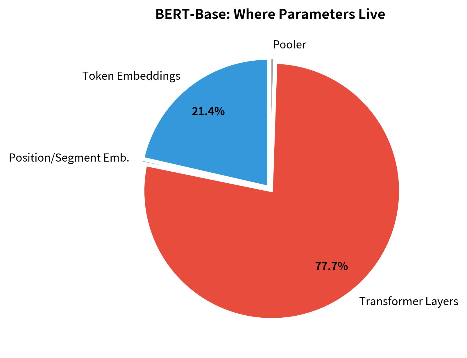
BERT's parameters concentrate in two places: the embedding layer and the transformer blocks. For BERT-Base with a vocabulary of approximately 30,000 tokens and hidden dimension of 768, the embedding matrix alone contains roughly 23 million parameters. That's about 21% of the model's total 110 million parameters, devoted entirely to a lookup table.

The embedding matrix size follows a simple formula: $V \times H$ , where $V$ is vocabulary size and $H$ is hidden dimension. This means larger vocabularies and wider models both inflate embedding costs linearly.

The transformer layers present a different kind of redundancy. Each of BERT's 12 layers has its own attention weights and feed-forward network, but researchers observed that layers often learn similar transformations. The question ALBERT asks: can we share parameters across layers without losing representation quality?

In[3]:

Code

def analyze_bert_parameters(
    vocab_size, hidden_size, num_layers, intermediate_size
):
    """Break down BERT's parameter distribution."""

    # Embedding parameters
    token_embeddings = vocab_size * hidden_size
    position_embeddings = 512 * hidden_size  # Max sequence length
    segment_embeddings = 2 * hidden_size
    embedding_layernorm = 2 * hidden_size
    total_embedding = (
        token_embeddings
        + position_embeddings
        + segment_embeddings
        + embedding_layernorm
    )

    # Per-layer transformer parameters
    # Self-attention: Q, K, V projections + output projection
    attention_params = (
        4 * hidden_size * hidden_size + 4 * hidden_size
    )  # weights + biases
    attention_layernorm = 2 * hidden_size

    # Feed-forward: two linear layers
    ffn_params = (
        hidden_size * intermediate_size + intermediate_size
    )  # First layer
    ffn_params += intermediate_size * hidden_size + hidden_size  # Second layer
    ffn_layernorm = 2 * hidden_size

    per_layer = (
        attention_params + attention_layernorm + ffn_params + ffn_layernorm
    )
    total_layers = num_layers * per_layer

    # Pooler (for classification)
    pooler = hidden_size * hidden_size + hidden_size

    total = total_embedding + total_layers + pooler

    return {
        "embedding": total_embedding,
        "per_layer": per_layer,
        "all_layers": total_layers,
        "pooler": pooler,
        "total": total,
        "embedding_pct": 100 * total_embedding / total,
        "layers_pct": 100 * total_layers / total,
    }

def analyze_bert_parameters(
    vocab_size, hidden_size, num_layers, intermediate_size
):
    """Break down BERT's parameter distribution."""

    # Embedding parameters
    token_embeddings = vocab_size * hidden_size
    position_embeddings = 512 * hidden_size  # Max sequence length
    segment_embeddings = 2 * hidden_size
    embedding_layernorm = 2 * hidden_size
    total_embedding = (
        token_embeddings
        + position_embeddings
        + segment_embeddings
        + embedding_layernorm
    )

    # Per-layer transformer parameters
    # Self-attention: Q, K, V projections + output projection
    attention_params = (
        4 * hidden_size * hidden_size + 4 * hidden_size
    )  # weights + biases
    attention_layernorm = 2 * hidden_size

    # Feed-forward: two linear layers
    ffn_params = (
        hidden_size * intermediate_size + intermediate_size
    )  # First layer
    ffn_params += intermediate_size * hidden_size + hidden_size  # Second layer
    ffn_layernorm = 2 * hidden_size

    per_layer = (
        attention_params + attention_layernorm + ffn_params + ffn_layernorm
    )
    total_layers = num_layers * per_layer

    # Pooler (for classification)
    pooler = hidden_size * hidden_size + hidden_size

    total = total_embedding + total_layers + pooler

    return {
        "embedding": total_embedding,
        "per_layer": per_layer,
        "all_layers": total_layers,
        "pooler": pooler,
        "total": total,
        "embedding_pct": 100 * total_embedding / total,
        "layers_pct": 100 * total_layers / total,
    }

Out[4]:

Console

BERT-Base Parameter Distribution:
  Embeddings: 23,837,184 (21.8%)
  Per transformer layer: 7,087,872
  All 12 layers: 85,054,464 (77.7%)
  Total: 109,482,240

Over 20% of parameters sit in embeddings, while the remaining ~80% are spread across transformer layers. ALBERT targets both sources of redundancy with separate techniques.

Out[5]:

Visualization

Pie chart showing BERT-Base parameter distribution between embeddings and transformer layers. — Parameter distribution in BERT-Base. Embeddings consume over 20% of parameters for a simple lookup operation, while transformer layers each contribute roughly equal amounts. ALBERT's factorized embeddings and cross-layer sharing target both sources.

Factorized Embedding ParameterizationLink Copied

BERT ties the embedding dimension directly to the hidden dimension. Every token maps to a 768-dimensional vector, which then flows through transformer layers of the same size. This seems natural, but it creates a problem: the embedding matrix grows with vocabulary size $V$ and hidden dimension $H$ , requiring $V \times H$ parameters.

Factorized Embeddings

A technique that decomposes the large embedding matrix into two smaller matrices. Instead of mapping tokens directly to hidden-size vectors ( $V \times H$ ), factorized embeddings first map to a smaller intermediate dimension ( $V \times E$ ), then project up to the hidden size ( $E \times H$ ). When $E \ll H$ , this dramatically reduces parameters.

ALBERT decouples these dimensions. Tokens first embed into a smaller space of dimension $E$ , then a linear projection maps them up to the hidden dimension $H$ . The parameter count changes from:

\text{Standard: } V \times H

to:

\text{Factorized: } V \times E + E \times H

where:

$V$ : vocabulary size (number of unique tokens the model can represent)
$H$ : hidden dimension (size of the representations flowing through transformer layers)
$E$ : embedding dimension (smaller intermediate dimension, typically 128)

The first term ( $V \times E$ ) represents the token-to-embedding lookup table. The second term ( $E \times H$ ) represents the projection matrix that expands embeddings to the hidden size. When $E \ll H$ , the factorization saves parameters because the expensive vocabulary-sized matrix uses the smaller dimension.

For BERT's vocabulary of 30,522 tokens, hidden size of 768, and an embedding dimension of 128:

\text{Standard: } 30,522 \times 768 = 23,440,896 \text{ parameters}

\text{Factorized: } 30,522 \times 128 + 128 \times 768 = 3,906,816 + 98,304 = 4,005,120 \text{ parameters}

That's an 83% reduction in embedding parameters with a single architectural change.

In[6]:

Code

class FactorizedEmbedding(nn.Module):
    """Factorized token embeddings as used in ALBERT."""

    def __init__(self, vocab_size, embedding_dim, hidden_dim):
        super().__init__()

        # First: tokens to small embedding space
        self.token_embedding = nn.Embedding(vocab_size, embedding_dim)

        # Second: project to hidden dimension
        self.projection = nn.Linear(embedding_dim, hidden_dim, bias=False)

    def forward(self, input_ids):
        # Embed tokens to small dimension
        x = self.token_embedding(input_ids)

        # Project to hidden dimension
        x = self.projection(x)

        return x

class FactorizedEmbedding(nn.Module):
    """Factorized token embeddings as used in ALBERT."""

    def __init__(self, vocab_size, embedding_dim, hidden_dim):
        super().__init__()

        # First: tokens to small embedding space
        self.token_embedding = nn.Embedding(vocab_size, embedding_dim)

        # Second: project to hidden dimension
        self.projection = nn.Linear(embedding_dim, hidden_dim, bias=False)

    def forward(self, input_ids):
        # Embed tokens to small dimension
        x = self.token_embedding(input_ids)

        # Project to hidden dimension
        x = self.projection(x)

        return x

Let's compare parameter counts:

In[7]:

Code

def compare_embedding_params(vocab_size, hidden_dim, embedding_dim):
    """Compare standard vs factorized embedding parameters."""

    standard_params = vocab_size * hidden_dim

    factorized_params = vocab_size * embedding_dim + embedding_dim * hidden_dim

    reduction = 1 - factorized_params / standard_params

    return {
        "standard": standard_params,
        "factorized": factorized_params,
        "reduction": reduction,
        "ratio": standard_params / factorized_params,
    }

def compare_embedding_params(vocab_size, hidden_dim, embedding_dim):
    """Compare standard vs factorized embedding parameters."""

    standard_params = vocab_size * hidden_dim

    factorized_params = vocab_size * embedding_dim + embedding_dim * hidden_dim

    reduction = 1 - factorized_params / standard_params

    return {
        "standard": standard_params,
        "factorized": factorized_params,
        "reduction": reduction,
        "ratio": standard_params / factorized_params,
    }

Out[8]:

Console

Embedding Parameter Comparison:
-----------------------------------------------------------------
BERT-Base (baseline)         |   24,030,720 params | -2.5% reduction
ALBERT-Base (E=128)          |    4,005,120 params | 82.9% reduction
ALBERT-Large (E=128)         |    4,037,888 params | 87.1% reduction
ALBERT-xLarge (E=128)        |    4,168,960 params | 93.3% reduction
ALBERT-xxLarge (E=128)       |    4,431,104 params | 96.5% reduction

The savings become more dramatic as hidden dimension increases. ALBERT-xxLarge with its 4096-dimensional hidden states would need 125 million embedding parameters under BERT's approach. Factorization reduces this to just 4.4 million.

Out[9]:

Visualization

Bar chart comparing standard vs factorized embedding parameters across ALBERT model sizes. — Embedding parameter reduction from factorization across model sizes. The savings grow with hidden dimension because the projection matrix ($E \times H$) grows linearly while the token matrix ($V \times E$) stays constant.

Why Factorization WorksLink Copied

At first glance, reducing embedding dimension seems like it would hurt representation quality. Tokens have less room to encode meaning. But the key insight is that embedding vectors and hidden states serve different purposes.

Token embeddings capture context-independent information. The embedding for "bank" is the same whether it appears in "river bank" or "savings bank." This relatively simple lookup doesn't require the full expressiveness of the hidden dimension, which must capture context-dependent representations built through multiple layers of attention.

In[10]:

Code

def demonstrate_projection_capacity():
    """Show that small embeddings project well to larger spaces."""
    torch.manual_seed(42)

    vocab_size = 1000
    embedding_dim = 64
    hidden_dim = 256

    # Create factorized embedding
    factorized = FactorizedEmbedding(vocab_size, embedding_dim, hidden_dim)

    # Sample some token IDs
    token_ids = torch.tensor([[0, 1, 2, 3, 4]])

    # Get intermediate and final representations
    intermediate = factorized.token_embedding(token_ids)
    final = factorized(token_ids)

    return intermediate, final

def demonstrate_projection_capacity():
    """Show that small embeddings project well to larger spaces."""
    torch.manual_seed(42)

    vocab_size = 1000
    embedding_dim = 64
    hidden_dim = 256

    # Create factorized embedding
    factorized = FactorizedEmbedding(vocab_size, embedding_dim, hidden_dim)

    # Sample some token IDs
    token_ids = torch.tensor([[0, 1, 2, 3, 4]])

    # Get intermediate and final representations
    intermediate = factorized.token_embedding(token_ids)
    final = factorized(token_ids)

    return intermediate, final

Out[11]:

Console

Representation Dimensions:
  Intermediate (E=64): torch.Size([1, 5, 64])
  After projection (H=256): torch.Size([1, 5, 256])

  Intermediate variance: 0.9986
  Final variance: 0.3171

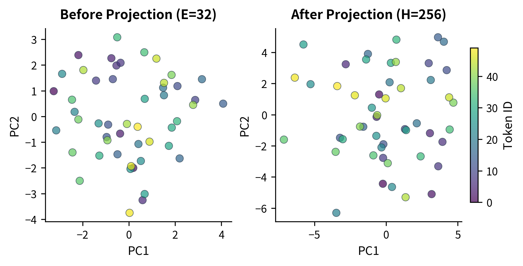
The intermediate representation is 4x smaller than the final output (64 vs 256 dimensions), yet it preserves the information needed for the projection layer to expand it. The variance change shows how the projection redistributes activation magnitudes across the larger hidden space.

The projection layer learns to expand the compressed representations into the full hidden space. During pretraining, this projection adapts to whatever patterns the model needs, effectively learning a task-appropriate decompression of the initial token representations.

We can visualize this by examining how different tokens map through the factorized embedding space:

Out[12]:

Visualization

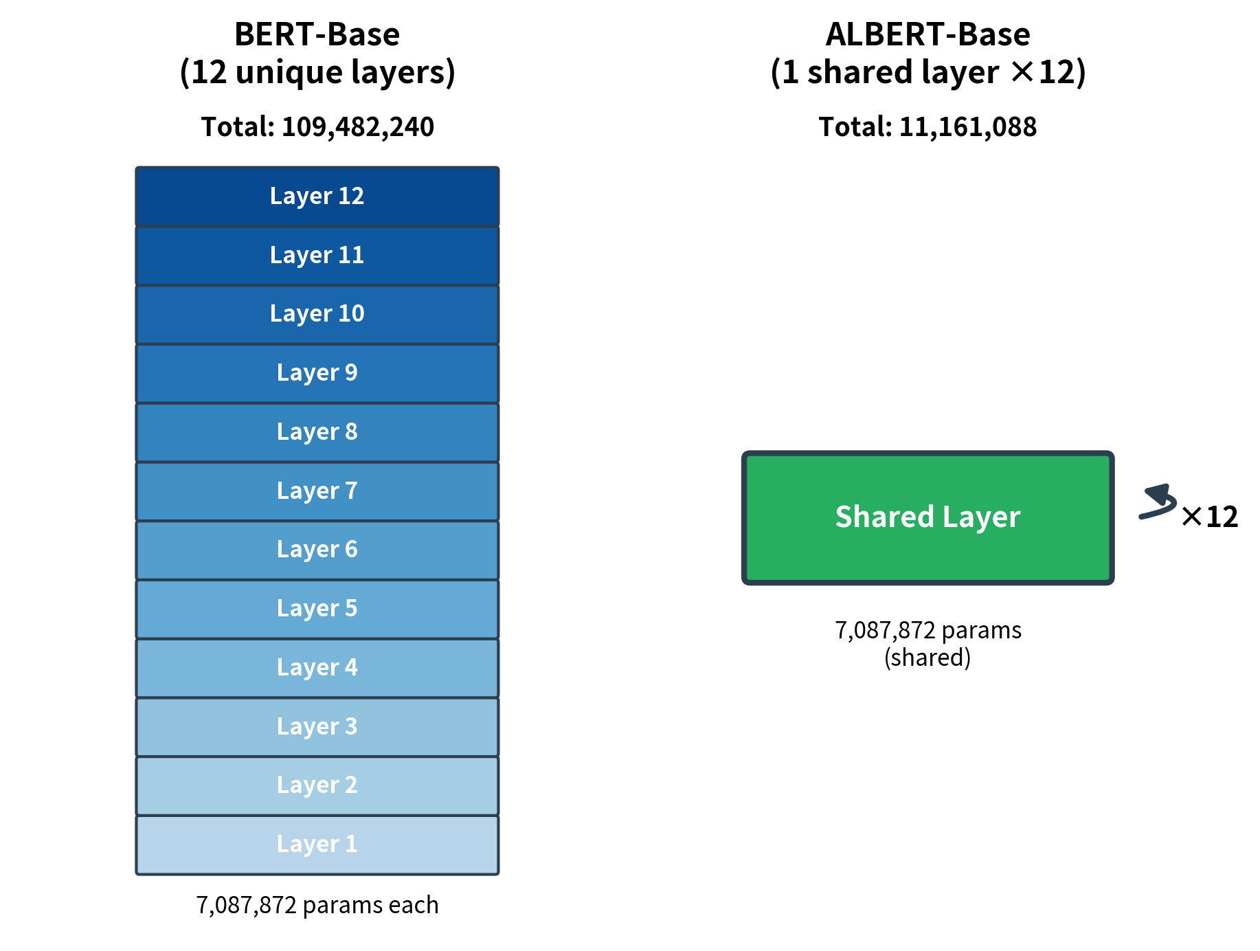
ALBERT's second major innovation is sharing parameters across transformer layers. Rather than each layer having its own attention and feed-forward weights, all layers share a single set of parameters. The model applies the same transformation repeatedly, with only the input changing between iterations.

Cross-Layer Parameter Sharing

A technique where transformer layers share the same weight matrices instead of learning independent parameters. This reduces model size proportionally to the number of layers while creating a form of iterative refinement where the same transformation is applied multiple times to progressively update representations.

This is a radical change. BERT-Base has 12 unique layers with 85 million combined parameters. ALBERT-Base has 12 layers but only one set of weights, reducing layer parameters by 12x.

In[13]:

Code

class SharedTransformerBlock(nn.Module):
    """A single transformer block that can be applied multiple times."""

    def __init__(self, hidden_dim, num_heads, intermediate_dim, dropout=0.1):
        super().__init__()

        # Multi-head self-attention
        self.attention = nn.MultiheadAttention(
            embed_dim=hidden_dim,
            num_heads=num_heads,
            dropout=dropout,
            batch_first=True,
        )
        self.attention_norm = nn.LayerNorm(hidden_dim)

        # Feed-forward network
        self.ffn = nn.Sequential(
            nn.Linear(hidden_dim, intermediate_dim),
            nn.GELU(),
            nn.Linear(intermediate_dim, hidden_dim),
            nn.Dropout(dropout),
        )
        self.ffn_norm = nn.LayerNorm(hidden_dim)

    def forward(self, x, attention_mask=None):
        # Self-attention with residual
        attn_out, _ = self.attention(x, x, x, key_padding_mask=attention_mask)
        x = self.attention_norm(x + attn_out)

        # FFN with residual
        ffn_out = self.ffn(x)
        x = self.ffn_norm(x + ffn_out)

        return x

class SharedTransformerBlock(nn.Module):
    """A single transformer block that can be applied multiple times."""

    def __init__(self, hidden_dim, num_heads, intermediate_dim, dropout=0.1):
        super().__init__()

        # Multi-head self-attention
        self.attention = nn.MultiheadAttention(
            embed_dim=hidden_dim,
            num_heads=num_heads,
            dropout=dropout,
            batch_first=True,
        )
        self.attention_norm = nn.LayerNorm(hidden_dim)

        # Feed-forward network
        self.ffn = nn.Sequential(
            nn.Linear(hidden_dim, intermediate_dim),
            nn.GELU(),
            nn.Linear(intermediate_dim, hidden_dim),
            nn.Dropout(dropout),
        )
        self.ffn_norm = nn.LayerNorm(hidden_dim)

    def forward(self, x, attention_mask=None):
        # Self-attention with residual
        attn_out, _ = self.attention(x, x, x, key_padding_mask=attention_mask)
        x = self.attention_norm(x + attn_out)

        # FFN with residual
        ffn_out = self.ffn(x)
        x = self.ffn_norm(x + ffn_out)

        return x

In[14]:

Code

class ALBERTEncoder(nn.Module):
    """ALBERT encoder with shared transformer layers."""

    def __init__(
        self,
        vocab_size,
        embedding_dim,
        hidden_dim,
        num_heads,
        intermediate_dim,
        num_layers,
        max_position=512,
        dropout=0.1,
    ):
        super().__init__()

        # Factorized embeddings
        self.token_embedding = nn.Embedding(vocab_size, embedding_dim)
        self.position_embedding = nn.Embedding(max_position, embedding_dim)
        self.segment_embedding = nn.Embedding(2, embedding_dim)

        # Project to hidden dimension
        self.embedding_projection = nn.Linear(embedding_dim, hidden_dim)
        self.embedding_norm = nn.LayerNorm(hidden_dim)
        self.embedding_dropout = nn.Dropout(dropout)

        # Single shared transformer block
        self.shared_layer = SharedTransformerBlock(
            hidden_dim, num_heads, intermediate_dim, dropout
        )

        self.num_layers = num_layers

    def forward(self, input_ids, segment_ids=None, attention_mask=None):
        batch_size, seq_len = input_ids.shape

        # Create position IDs
        positions = torch.arange(seq_len, device=input_ids.device).unsqueeze(0)

        # Get embeddings
        x = self.token_embedding(input_ids)
        x = x + self.position_embedding(positions)
        if segment_ids is not None:
            x = x + self.segment_embedding(segment_ids)

        # Project to hidden dimension
        x = self.embedding_projection(x)
        x = self.embedding_norm(x)
        x = self.embedding_dropout(x)

        # Apply shared layer multiple times
        for _ in range(self.num_layers):
            x = self.shared_layer(x, attention_mask)

        return x

class ALBERTEncoder(nn.Module):
    """ALBERT encoder with shared transformer layers."""

    def __init__(
        self,
        vocab_size,
        embedding_dim,
        hidden_dim,
        num_heads,
        intermediate_dim,
        num_layers,
        max_position=512,
        dropout=0.1,
    ):
        super().__init__()

        # Factorized embeddings
        self.token_embedding = nn.Embedding(vocab_size, embedding_dim)
        self.position_embedding = nn.Embedding(max_position, embedding_dim)
        self.segment_embedding = nn.Embedding(2, embedding_dim)

        # Project to hidden dimension
        self.embedding_projection = nn.Linear(embedding_dim, hidden_dim)
        self.embedding_norm = nn.LayerNorm(hidden_dim)
        self.embedding_dropout = nn.Dropout(dropout)

        # Single shared transformer block
        self.shared_layer = SharedTransformerBlock(
            hidden_dim, num_heads, intermediate_dim, dropout
        )

        self.num_layers = num_layers

    def forward(self, input_ids, segment_ids=None, attention_mask=None):
        batch_size, seq_len = input_ids.shape

        # Create position IDs
        positions = torch.arange(seq_len, device=input_ids.device).unsqueeze(0)

        # Get embeddings
        x = self.token_embedding(input_ids)
        x = x + self.position_embedding(positions)
        if segment_ids is not None:
            x = x + self.segment_embedding(segment_ids)

        # Project to hidden dimension
        x = self.embedding_projection(x)
        x = self.embedding_norm(x)
        x = self.embedding_dropout(x)

        # Apply shared layer multiple times
        for _ in range(self.num_layers):
            x = self.shared_layer(x, attention_mask)

        return x

Let's compare the parameter counts:

In[15]:

Code

def count_parameters(model):
    """Count trainable parameters in a model."""
    return sum(p.numel() for p in model.parameters() if p.requires_grad)


# Create ALBERT-style encoder
torch.manual_seed(42)
albert_encoder = ALBERTEncoder(
    vocab_size=30522,
    embedding_dim=128,
    hidden_dim=768,
    num_heads=12,
    intermediate_dim=3072,
    num_layers=12,
)

def count_parameters(model):
    """Count trainable parameters in a model."""
    return sum(p.numel() for p in model.parameters() if p.requires_grad)


# Create ALBERT-style encoder
torch.manual_seed(42)
albert_encoder = ALBERTEncoder(
    vocab_size=30522,
    embedding_dim=128,
    hidden_dim=768,
    num_heads=12,
    intermediate_dim=3072,
    num_layers=12,
)

Out[16]:

Console

Parameter Comparison (12 layers):
  BERT-Base:   109,482,240 parameters
  ALBERT-Base:   11,161,088 parameters
  Reduction: 89.8%

ALBERT-Base Parameter Breakdown:
  Embeddings + projection: 4,073,216
  Shared transformer layer: 7,087,872
  Total: 11,161,088

The parameter reduction is dramatic. ALBERT-Base achieves roughly 89% fewer parameters than BERT-Base while maintaining the same number of computational steps (12 layer applications).

Out[17]:

Visualization

Side-by-side comparison showing BERT with 12 unique layers versus ALBERT with 1 shared layer applied 12 times. — Parameter distribution in BERT vs ALBERT. BERT dedicates unique parameters to each layer, while ALBERT reuses a single layer's parameters. Both models perform the same number of forward pass computations.

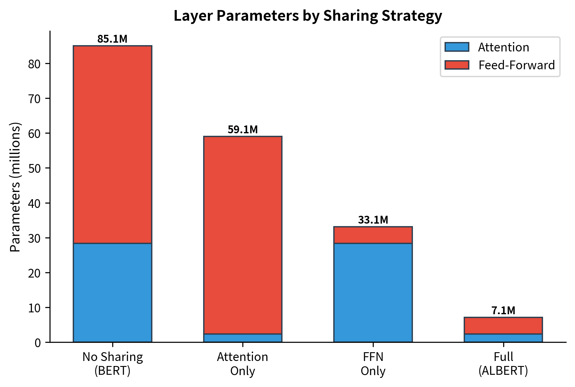
ALBERT's paper explored several sharing strategies beyond full sharing. You can share only attention parameters, only feed-forward parameters, or share everything. The experiments revealed that full sharing works surprisingly well.

In[18]:

Code

def compare_sharing_strategies(
    hidden_dim, num_heads, intermediate_dim, num_layers
):
    """Compare parameter counts under different sharing strategies."""

    # Per-layer component sizes
    attention_params = (
        4 * hidden_dim * hidden_dim + 4 * hidden_dim
    )  # Q,K,V,O projections
    attention_norm = 2 * hidden_dim
    ffn_params = (
        hidden_dim * intermediate_dim + intermediate_dim
    )  # Up projection
    ffn_params += intermediate_dim * hidden_dim + hidden_dim  # Down projection
    ffn_norm = 2 * hidden_dim

    attention_total = attention_params + attention_norm
    ffn_total = ffn_params + ffn_norm
    layer_total = attention_total + ffn_total

    strategies = {
        "No sharing (BERT)": {
            "attention": attention_total * num_layers,
            "ffn": ffn_total * num_layers,
        },
        "Share attention only": {
            "attention": attention_total,  # Shared
            "ffn": ffn_total * num_layers,  # Unique
        },
        "Share FFN only": {
            "attention": attention_total * num_layers,  # Unique
            "ffn": ffn_total,  # Shared
        },
        "Share all (ALBERT)": {
            "attention": attention_total,  # Shared
            "ffn": ffn_total,  # Shared
        },
    }

    for name, params in strategies.items():
        params["total"] = params["attention"] + params["ffn"]

    return strategies, layer_total * num_layers

def compare_sharing_strategies(
    hidden_dim, num_heads, intermediate_dim, num_layers
):
    """Compare parameter counts under different sharing strategies."""

    # Per-layer component sizes
    attention_params = (
        4 * hidden_dim * hidden_dim + 4 * hidden_dim
    )  # Q,K,V,O projections
    attention_norm = 2 * hidden_dim
    ffn_params = (
        hidden_dim * intermediate_dim + intermediate_dim
    )  # Up projection
    ffn_params += intermediate_dim * hidden_dim + hidden_dim  # Down projection
    ffn_norm = 2 * hidden_dim

    attention_total = attention_params + attention_norm
    ffn_total = ffn_params + ffn_norm
    layer_total = attention_total + ffn_total

    strategies = {
        "No sharing (BERT)": {
            "attention": attention_total * num_layers,
            "ffn": ffn_total * num_layers,
        },
        "Share attention only": {
            "attention": attention_total,  # Shared
            "ffn": ffn_total * num_layers,  # Unique
        },
        "Share FFN only": {
            "attention": attention_total * num_layers,  # Unique
            "ffn": ffn_total,  # Shared
        },
        "Share all (ALBERT)": {
            "attention": attention_total,  # Shared
            "ffn": ffn_total,  # Shared
        },
    }

    for name, params in strategies.items():
        params["total"] = params["attention"] + params["ffn"]

    return strategies, layer_total * num_layers

Out[19]:

Console

Layer Parameter Comparison (hidden=768, 12 layers):
-------------------------------------------------------
No sharing (BERT)         | 85,054,464 |   0.0% reduction
Share attention only      | 59,051,520 |  30.6% reduction
Share FFN only            | 33,090,816 |  61.1% reduction
Share all (ALBERT)        |  7,087,872 |  91.7% reduction

Full sharing provides the largest reduction. The ALBERT paper showed that performance degradation from sharing was minimal, particularly for the feed-forward layers. Attention sharing has slightly more impact because different layers benefit from attending to different aspects of the input.

Out[20]:

Visualization

Bar chart comparing parameter counts across four sharing strategies. — Parameter counts under different sharing strategies. Sharing only attention or only FFN provides partial savings. Full sharing, as used in ALBERT, maximizes parameter reduction while maintaining competitive performance.

Iterative RefinementLink Copied

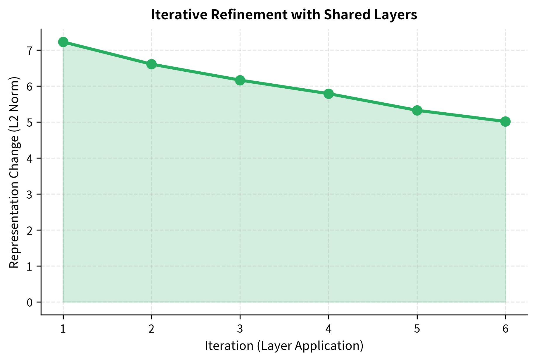
Cross-layer sharing creates an interesting computational pattern. Instead of passing through 12 different transformations, the input passes through the same transformation 12 times. Each iteration refines the representation, similar to how iterative algorithms converge toward a solution.

In[21]:

Code

def track_layer_representations(model, input_ids):
    """Track how representations evolve through repeated layer applications."""

    batch_size, seq_len = input_ids.shape
    positions = torch.arange(seq_len, device=input_ids.device).unsqueeze(0)

    # Get initial embeddings
    x = model.token_embedding(input_ids)
    x = x + model.position_embedding(positions)
    x = model.embedding_projection(x)
    x = model.embedding_norm(x)

    # Track representations at each iteration
    representations = [x.detach().clone()]

    for i in range(model.num_layers):
        x = model.shared_layer(x)
        representations.append(x.detach().clone())

    return representations

def track_layer_representations(model, input_ids):
    """Track how representations evolve through repeated layer applications."""

    batch_size, seq_len = input_ids.shape
    positions = torch.arange(seq_len, device=input_ids.device).unsqueeze(0)

    # Get initial embeddings
    x = model.token_embedding(input_ids)
    x = x + model.position_embedding(positions)
    x = model.embedding_projection(x)
    x = model.embedding_norm(x)

    # Track representations at each iteration
    representations = [x.detach().clone()]

    for i in range(model.num_layers):
        x = model.shared_layer(x)
        representations.append(x.detach().clone())

    return representations

In[22]:

Code

# Create a small model for visualization
torch.manual_seed(42)
small_albert = ALBERTEncoder(
    vocab_size=1000,
    embedding_dim=32,
    hidden_dim=64,
    num_heads=4,
    intermediate_dim=128,
    num_layers=6,
)

# Random input
input_ids = torch.randint(0, 1000, (1, 10))
representations = track_layer_representations(small_albert, input_ids)

# Create a small model for visualization
torch.manual_seed(42)
small_albert = ALBERTEncoder(
    vocab_size=1000,
    embedding_dim=32,
    hidden_dim=64,
    num_heads=4,
    intermediate_dim=128,
    num_layers=6,
)

# Random input
input_ids = torch.randint(0, 1000, (1, 10))
representations = track_layer_representations(small_albert, input_ids)

Out[23]:

Console

Representation Change Between Iterations:
  Iteration 0 → 1: 7.2268
  Iteration 1 → 2: 6.6079
  Iteration 2 → 3: 6.1655
  Iteration 3 → 4: 5.7893
  Iteration 4 → 5: 5.3263
  Iteration 5 → 6: 5.0161

The representation changes decrease across iterations, indicating that repeated applications of the same layer produce diminishing modifications. This convergence-like behavior suggests the model is iteratively refining toward a stable representation rather than making dramatic changes at each step.

We can visualize how similar representations are across iterations using cosine similarity. If shared layers truly perform iterative refinement, we should see adjacent iterations being more similar than distant ones:

Out[24]:

Visualization

Heatmap showing cosine similarity matrix between representations at each layer iteration. — Cosine similarity between representations at different iterations. Adjacent iterations show high similarity (dark colors along the diagonal), while early and late iterations are less similar. This pattern confirms the iterative refinement hypothesis: each layer application makes incremental adjustments rather than wholesale changes.

Out[25]:

Visualization

Line plot showing representation change magnitude decreasing across iterations. — Representation change across layer iterations. With shared parameters, each application of the layer produces progressively smaller changes, suggesting convergence toward a stable representation. This pattern differs from BERT, where each layer can produce arbitrarily different transformations.

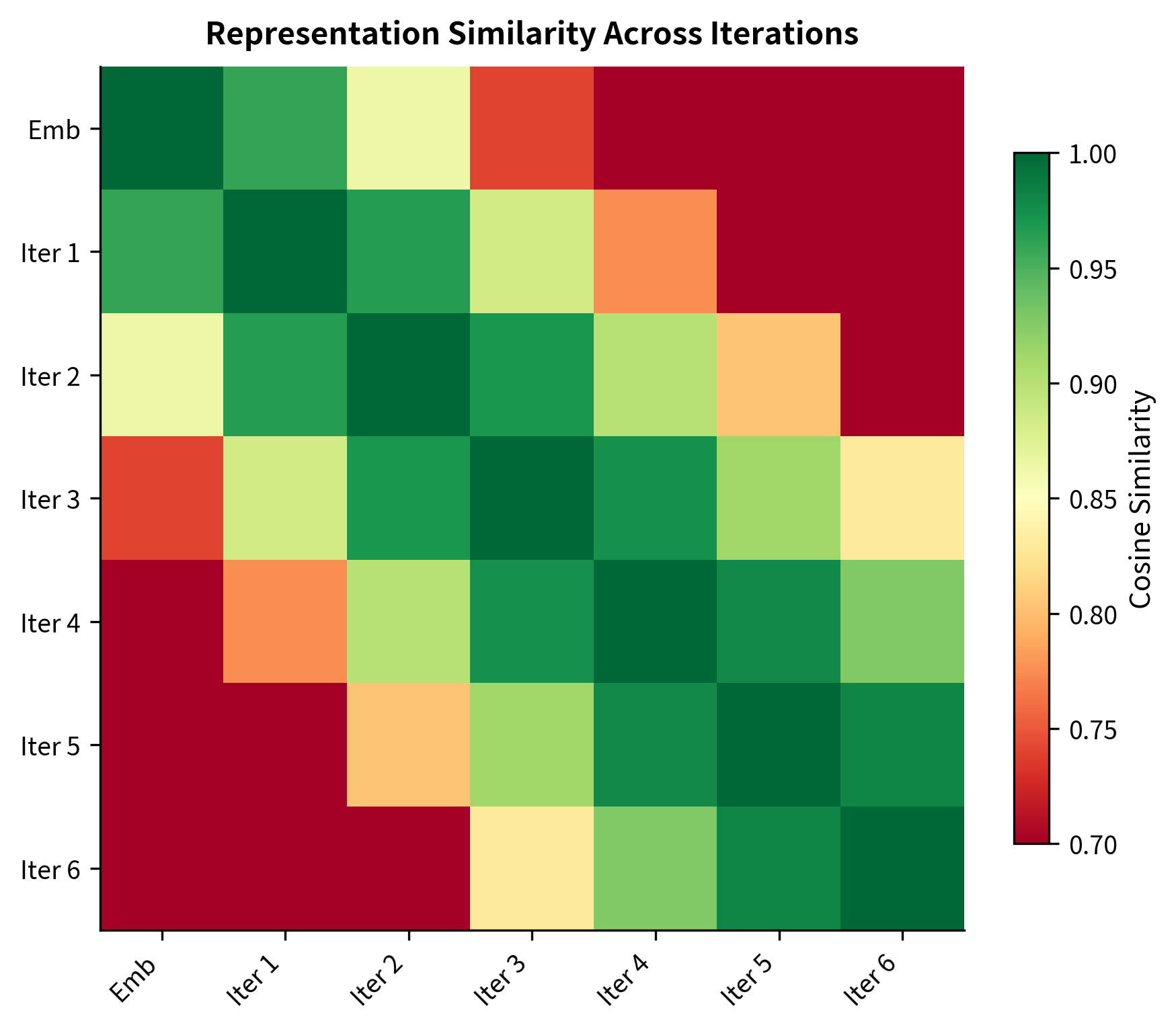
This iterative behavior has theoretical connections to fixed-point computation and recurrent neural networks. The shared layer learns a single step of refinement, and multiple applications accumulate into a complete transformation.

Sentence Order PredictionLink Copied

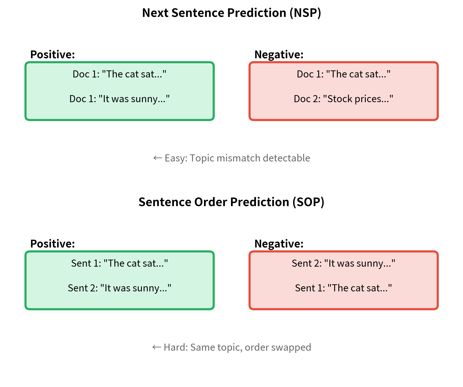
BERT's Next Sentence Prediction (NSP) task asked whether two sentences appeared consecutively in the original document. Critics argued this task was too easy: the model could often succeed by detecting topic consistency rather than understanding inter-sentence coherence.

ALBERT replaced NSP with Sentence Order Prediction (SOP), a harder task. Given two consecutive sentences, SOP asks whether they appear in the correct order or have been swapped.

Sentence Order Prediction (SOP)

A pretraining task where the model predicts whether two consecutive sentences appear in their original order or have been swapped. Unlike Next Sentence Prediction, SOP requires understanding discourse coherence since both sentences come from the same document and share the same topic.

In[26]:

Code

def create_sop_examples(sentences, positive_ratio=0.5):
    """Create sentence order prediction training examples."""

    examples = []
    labels = []

    for i in range(len(sentences) - 1):
        sent_a = sentences[i]
        sent_b = sentences[i + 1]

        # Randomly decide: positive (correct order) or negative (swapped)
        if np.random.random() < positive_ratio:
            # Correct order
            examples.append((sent_a, sent_b))
            labels.append(1)  # Is in correct order
        else:
            # Swapped order
            examples.append((sent_b, sent_a))
            labels.append(0)  # Not in correct order

    return examples, labels

def create_sop_examples(sentences, positive_ratio=0.5):
    """Create sentence order prediction training examples."""

    examples = []
    labels = []

    for i in range(len(sentences) - 1):
        sent_a = sentences[i]
        sent_b = sentences[i + 1]

        # Randomly decide: positive (correct order) or negative (swapped)
        if np.random.random() < positive_ratio:
            # Correct order
            examples.append((sent_a, sent_b))
            labels.append(1)  # Is in correct order
        else:
            # Swapped order
            examples.append((sent_b, sent_a))
            labels.append(0)  # Not in correct order

    return examples, labels

In[27]:

Code

# Example sentences from a document
document_sentences = [
    "The cat sat on the mat.",
    "It was a sunny afternoon.",
    "Birds chirped in the nearby tree.",
    "The cat watched them lazily.",
    "Eventually, it fell asleep.",
]

np.random.seed(42)
examples, labels = create_sop_examples(document_sentences, positive_ratio=0.5)

# Example sentences from a document
document_sentences = [
    "The cat sat on the mat.",
    "It was a sunny afternoon.",
    "Birds chirped in the nearby tree.",
    "The cat watched them lazily.",
    "Eventually, it fell asleep.",
]

np.random.seed(42)
examples, labels = create_sop_examples(document_sentences, positive_ratio=0.5)

Out[28]:

Console

Sentence Order Prediction Examples:
------------------------------------------------------------

Example 1 (Correct):
  Sentence A: The cat sat on the mat.
  Sentence B: It was a sunny afternoon.

Example 2 (Swapped):
  Sentence A: Birds chirped in the nearby tree.
  Sentence B: It was a sunny afternoon.

Example 3 (Swapped):
  Sentence A: The cat watched them lazily.
  Sentence B: Birds chirped in the nearby tree.

Example 4 (Swapped):
  Sentence A: Eventually, it fell asleep.
  Sentence B: The cat watched them lazily.

SOP is harder than NSP because both sentences always come from the same document. The model cannot rely on topic mismatch to detect negatives. Instead, it must understand temporal and logical relationships between sentences. Does "It fell asleep" make sense before "It watched them lazily"? Only genuine discourse understanding can answer that.

Out[29]:

Visualization

Diagram contrasting NSP and SOP task construction with positive and negative examples. — Comparison of NSP and SOP pretraining tasks. NSP negatives come from different documents, making topic detection sufficient. SOP negatives are sentence swaps within the same document, requiring discourse-level understanding of sentence relationships.

Implementing a Complete ALBERT ModelLink Copied

Let's put together factorized embeddings, shared layers, and the SOP classification head into a complete ALBERT model.

In[30]:

Code

class ALBERT(nn.Module):
    """Complete ALBERT model with factorized embeddings and shared layers."""

    def __init__(
        self,
        vocab_size=30522,
        embedding_dim=128,
        hidden_dim=768,
        num_heads=12,
        intermediate_dim=3072,
        num_layers=12,
        max_position=512,
        dropout=0.1,
    ):
        super().__init__()

        self.hidden_dim = hidden_dim

        # Factorized embeddings
        self.token_embedding = nn.Embedding(vocab_size, embedding_dim)
        self.position_embedding = nn.Embedding(max_position, embedding_dim)
        self.segment_embedding = nn.Embedding(2, embedding_dim)

        # Projection to hidden dimension
        self.embedding_projection = nn.Linear(embedding_dim, hidden_dim)
        self.embedding_norm = nn.LayerNorm(hidden_dim)
        self.embedding_dropout = nn.Dropout(dropout)

        # Single shared transformer block
        self.shared_layer = SharedTransformerBlock(
            hidden_dim, num_heads, intermediate_dim, dropout
        )
        self.num_layers = num_layers

        # Pooler for sentence-level representations
        self.pooler = nn.Sequential(
            nn.Linear(hidden_dim, hidden_dim), nn.Tanh()
        )

        # MLM head (shares embedding weights for output projection)
        self.mlm_dense = nn.Linear(hidden_dim, embedding_dim)
        self.mlm_norm = nn.LayerNorm(embedding_dim)
        self.mlm_decoder = nn.Linear(embedding_dim, vocab_size)
        # Weight tying: reuse token embeddings for output
        self.mlm_decoder.weight = self.token_embedding.weight

        # SOP head
        self.sop_classifier = nn.Linear(hidden_dim, 2)

    def forward(self, input_ids, segment_ids=None, attention_mask=None):
        batch_size, seq_len = input_ids.shape

        # Create position IDs
        positions = torch.arange(seq_len, device=input_ids.device).unsqueeze(0)

        # Embeddings
        x = self.token_embedding(input_ids)
        x = x + self.position_embedding(positions)
        if segment_ids is not None:
            x = x + self.segment_embedding(segment_ids)

        # Project and normalize
        x = self.embedding_projection(x)
        x = self.embedding_norm(x)
        x = self.embedding_dropout(x)

        # Apply shared layer multiple times
        for _ in range(self.num_layers):
            x = self.shared_layer(x, attention_mask)

        # Sequence output
        sequence_output = x

        # Pooled output from [CLS] token (position 0)
        pooled_output = self.pooler(x[:, 0])

        return sequence_output, pooled_output

    def get_mlm_logits(self, sequence_output):
        """Get masked language modeling predictions."""
        x = self.mlm_dense(sequence_output)
        x = F.gelu(x)
        x = self.mlm_norm(x)
        logits = self.mlm_decoder(x)
        return logits

    def get_sop_logits(self, pooled_output):
        """Get sentence order prediction logits."""
        return self.sop_classifier(pooled_output)

class ALBERT(nn.Module):
    """Complete ALBERT model with factorized embeddings and shared layers."""

    def __init__(
        self,
        vocab_size=30522,
        embedding_dim=128,
        hidden_dim=768,
        num_heads=12,
        intermediate_dim=3072,
        num_layers=12,
        max_position=512,
        dropout=0.1,
    ):
        super().__init__()

        self.hidden_dim = hidden_dim

        # Factorized embeddings
        self.token_embedding = nn.Embedding(vocab_size, embedding_dim)
        self.position_embedding = nn.Embedding(max_position, embedding_dim)
        self.segment_embedding = nn.Embedding(2, embedding_dim)

        # Projection to hidden dimension
        self.embedding_projection = nn.Linear(embedding_dim, hidden_dim)
        self.embedding_norm = nn.LayerNorm(hidden_dim)
        self.embedding_dropout = nn.Dropout(dropout)

        # Single shared transformer block
        self.shared_layer = SharedTransformerBlock(
            hidden_dim, num_heads, intermediate_dim, dropout
        )
        self.num_layers = num_layers

        # Pooler for sentence-level representations
        self.pooler = nn.Sequential(
            nn.Linear(hidden_dim, hidden_dim), nn.Tanh()
        )

        # MLM head (shares embedding weights for output projection)
        self.mlm_dense = nn.Linear(hidden_dim, embedding_dim)
        self.mlm_norm = nn.LayerNorm(embedding_dim)
        self.mlm_decoder = nn.Linear(embedding_dim, vocab_size)
        # Weight tying: reuse token embeddings for output
        self.mlm_decoder.weight = self.token_embedding.weight

        # SOP head
        self.sop_classifier = nn.Linear(hidden_dim, 2)

    def forward(self, input_ids, segment_ids=None, attention_mask=None):
        batch_size, seq_len = input_ids.shape

        # Create position IDs
        positions = torch.arange(seq_len, device=input_ids.device).unsqueeze(0)

        # Embeddings
        x = self.token_embedding(input_ids)
        x = x + self.position_embedding(positions)
        if segment_ids is not None:
            x = x + self.segment_embedding(segment_ids)

        # Project and normalize
        x = self.embedding_projection(x)
        x = self.embedding_norm(x)
        x = self.embedding_dropout(x)

        # Apply shared layer multiple times
        for _ in range(self.num_layers):
            x = self.shared_layer(x, attention_mask)

        # Sequence output
        sequence_output = x

        # Pooled output from [CLS] token (position 0)
        pooled_output = self.pooler(x[:, 0])

        return sequence_output, pooled_output

    def get_mlm_logits(self, sequence_output):
        """Get masked language modeling predictions."""
        x = self.mlm_dense(sequence_output)
        x = F.gelu(x)
        x = self.mlm_norm(x)
        logits = self.mlm_decoder(x)
        return logits

    def get_sop_logits(self, pooled_output):
        """Get sentence order prediction logits."""
        return self.sop_classifier(pooled_output)

In[31]:

Code

# Create model and test
torch.manual_seed(42)
albert = ALBERT(
    vocab_size=30522,
    embedding_dim=128,
    hidden_dim=768,
    num_heads=12,
    intermediate_dim=3072,
    num_layers=12,
)

# Random input
input_ids = torch.randint(0, 30522, (2, 64))
segment_ids = torch.zeros_like(input_ids)
segment_ids[:, 32:] = 1  # Second half is segment B

sequence_output, pooled_output = albert(input_ids, segment_ids)
mlm_logits = albert.get_mlm_logits(sequence_output)
sop_logits = albert.get_sop_logits(pooled_output)

# Create model and test
torch.manual_seed(42)
albert = ALBERT(
    vocab_size=30522,
    embedding_dim=128,
    hidden_dim=768,
    num_heads=12,
    intermediate_dim=3072,
    num_layers=12,
)

# Random input
input_ids = torch.randint(0, 30522, (2, 64))
segment_ids = torch.zeros_like(input_ids)
segment_ids[:, 32:] = 1  # Second half is segment B

sequence_output, pooled_output = albert(input_ids, segment_ids)
mlm_logits = albert.get_mlm_logits(sequence_output)
sop_logits = albert.get_sop_logits(pooled_output)

Out[32]:

Console

ALBERT Model Summary:
  Total parameters: 11,882,428
  Sequence output shape: torch.Size([2, 64, 768])
  Pooled output shape: torch.Size([2, 768])
  MLM logits shape: torch.Size([2, 64, 30522])
  SOP logits shape: torch.Size([2, 2])

Parameter comparison:
  BERT-Base: 109.5M parameters
  ALBERT-Base: 11.9M parameters
  Reduction: 89.1%

ALBERT Model ConfigurationsLink Copied

The original paper introduced four model sizes. Unlike BERT, which scaled parameters with layers, ALBERT scales the hidden dimension while keeping shared parameters.

In[33]:

Code

albert_configs = {
    "ALBERT-Base": {
        "embedding_dim": 128,
        "hidden_dim": 768,
        "num_heads": 12,
        "intermediate_dim": 3072,
        "num_layers": 12,
    },
    "ALBERT-Large": {
        "embedding_dim": 128,
        "hidden_dim": 1024,
        "num_heads": 16,
        "intermediate_dim": 4096,
        "num_layers": 24,
    },
    "ALBERT-xLarge": {
        "embedding_dim": 128,
        "hidden_dim": 2048,
        "num_heads": 16,
        "intermediate_dim": 8192,
        "num_layers": 24,
    },
    "ALBERT-xxLarge": {
        "embedding_dim": 128,
        "hidden_dim": 4096,
        "num_heads": 64,
        "intermediate_dim": 16384,
        "num_layers": 12,
    },
}


def estimate_albert_params(config, vocab_size=30522):
    """Estimate parameter count for an ALBERT configuration."""
    e = config["embedding_dim"]
    h = config["hidden_dim"]
    i = config["intermediate_dim"]
    heads = config["num_heads"]

    # Factorized embeddings
    embedding_params = (
        vocab_size * e + 512 * e + 2 * e
    )  # Token, position, segment
    projection_params = e * h  # Embed projection

    # Shared layer (only counted once)
    attention_params = 4 * h * h + 4 * h  # Q, K, V, O
    ffn_params = h * i + i + i * h + h  # Two layers with biases
    layer_params = attention_params + ffn_params + 4 * h  # Plus LayerNorms

    # Heads
    mlm_head = (
        h * e + e + 2 * e + vocab_size * e
    )  # Dense + norm + decoder (tied)
    sop_head = h * 2
    pooler = h * h + h

    total = (
        embedding_params
        + projection_params
        + layer_params
        + mlm_head
        + sop_head
        + pooler
    )

    return total

albert_configs = {
    "ALBERT-Base": {
        "embedding_dim": 128,
        "hidden_dim": 768,
        "num_heads": 12,
        "intermediate_dim": 3072,
        "num_layers": 12,
    },
    "ALBERT-Large": {
        "embedding_dim": 128,
        "hidden_dim": 1024,
        "num_heads": 16,
        "intermediate_dim": 4096,
        "num_layers": 24,
    },
    "ALBERT-xLarge": {
        "embedding_dim": 128,
        "hidden_dim": 2048,
        "num_heads": 16,
        "intermediate_dim": 8192,
        "num_layers": 24,
    },
    "ALBERT-xxLarge": {
        "embedding_dim": 128,
        "hidden_dim": 4096,
        "num_heads": 64,
        "intermediate_dim": 16384,
        "num_layers": 12,
    },
}


def estimate_albert_params(config, vocab_size=30522):
    """Estimate parameter count for an ALBERT configuration."""
    e = config["embedding_dim"]
    h = config["hidden_dim"]
    i = config["intermediate_dim"]
    heads = config["num_heads"]

    # Factorized embeddings
    embedding_params = (
        vocab_size * e + 512 * e + 2 * e
    )  # Token, position, segment
    projection_params = e * h  # Embed projection

    # Shared layer (only counted once)
    attention_params = 4 * h * h + 4 * h  # Q, K, V, O
    ffn_params = h * i + i + i * h + h  # Two layers with biases
    layer_params = attention_params + ffn_params + 4 * h  # Plus LayerNorms

    # Heads
    mlm_head = (
        h * e + e + 2 * e + vocab_size * e
    )  # Dense + norm + decoder (tied)
    sop_head = h * 2
    pooler = h * h + h

    total = (
        embedding_params
        + projection_params
        + layer_params
        + mlm_head
        + sop_head
        + pooler
    )

    return total

Out[34]:

Console

ALBERT Model Configurations:
---------------------------------------------------------------------------
Model              Hidden   Layers   Intermediate   Est. Params 
---------------------------------------------------------------------------
ALBERT-Base        768      12       3072               15.8M
ALBERT-Large       1024     24       4096               21.8M
ALBERT-xLarge      2048     24       8192               63.0M
ALBERT-xxLarge     4096     12       16384             227.1M

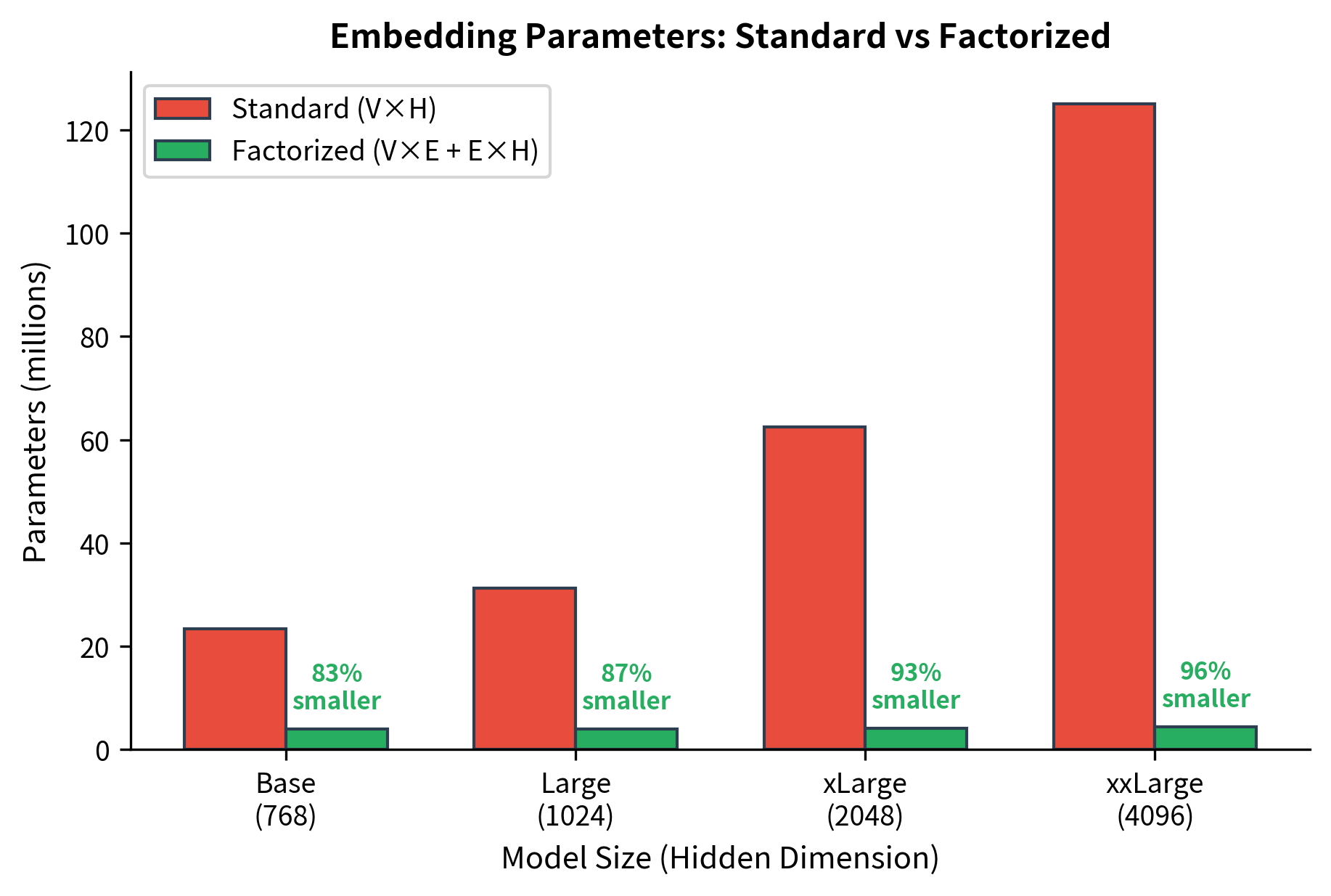
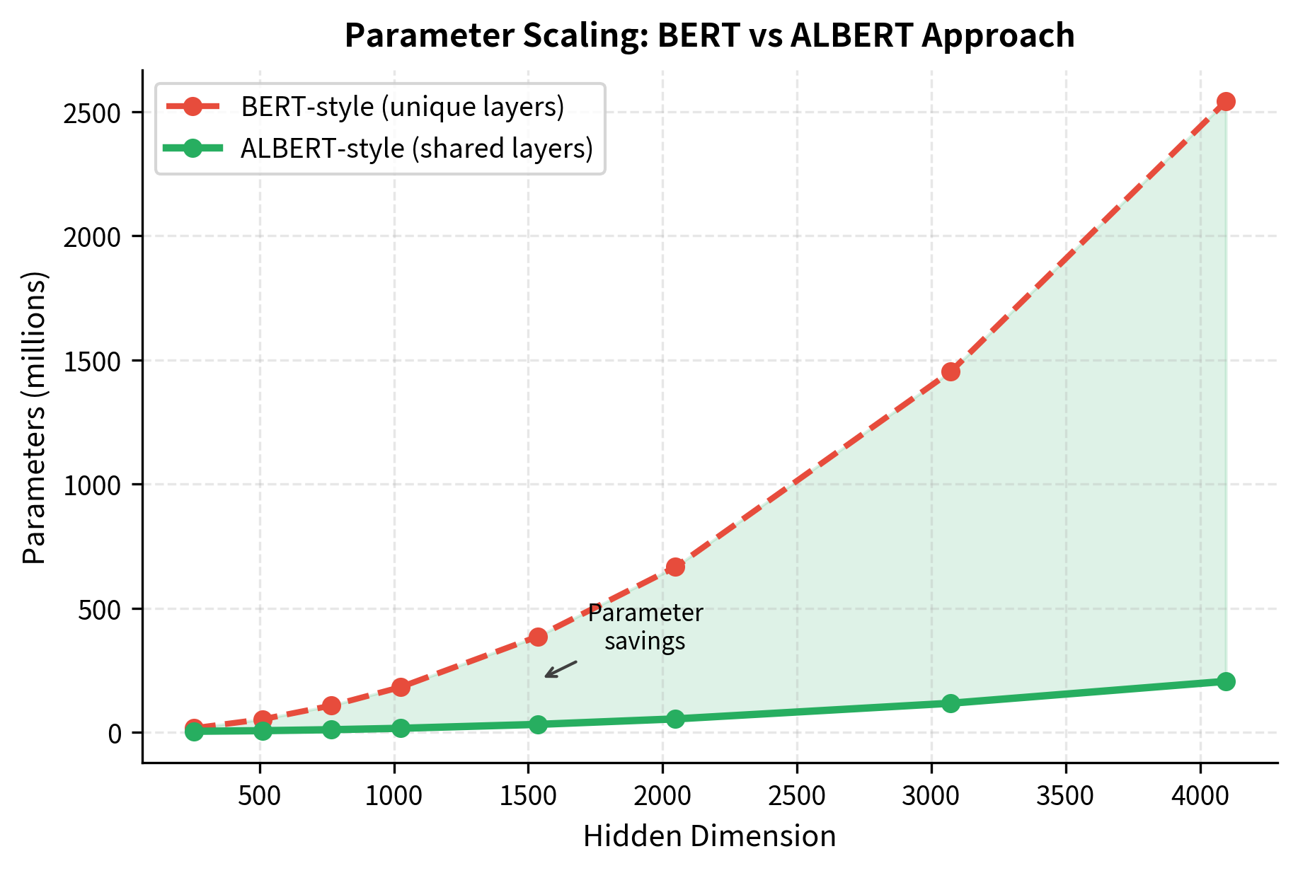
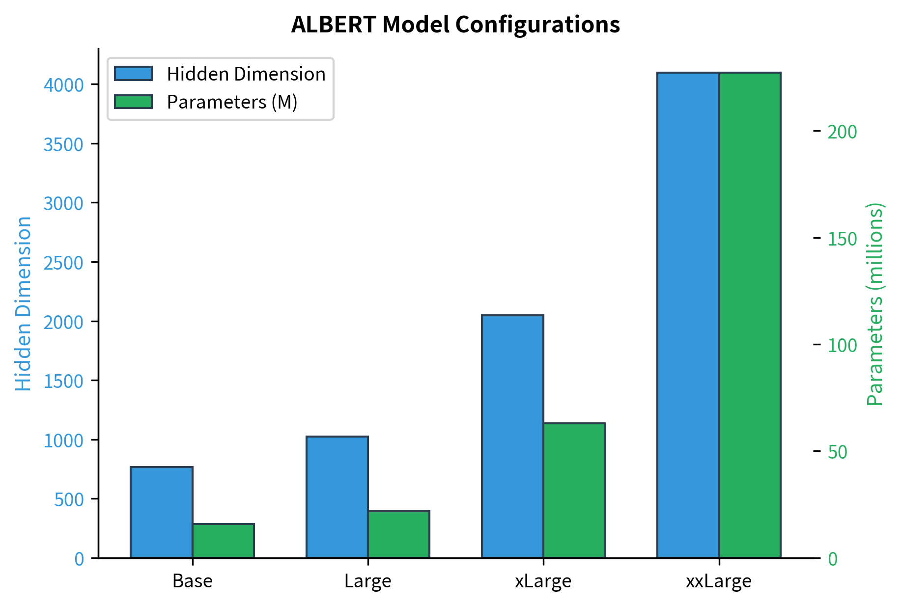
Notice how parameter counts grow much slower than hidden dimensions. ALBERT-xxLarge has a hidden dimension 5.3x larger than ALBERT-Base (4096 vs 768), but its parameter count is only about 20x larger. With BERT's approach, the parameter ratio would match the hidden dimension ratio squared, since attention parameters scale with $H^2$ .

The largest model, ALBERT-xxLarge, uses only 12 layers but has a massive 4096-dimensional hidden space. This reflects the finding that wider models with shared parameters can match deeper models with unique parameters.

We can visualize how differently parameters scale between BERT's approach and ALBERT's:

Out[35]:

Visualization

Line plot comparing parameter growth for BERT-style vs ALBERT-style scaling across hidden dimensions. — Parameter scaling with hidden dimension. BERT-style models (dashed) scale quadratically with hidden dimension because each layer has unique attention weights. ALBERT (solid) grows much more slowly because only one layer's worth of attention parameters exists, regardless of depth.

Out[36]:

Visualization

Bar chart comparing hidden dimensions and estimated parameters across ALBERT model sizes. — ALBERT configuration comparison. While hidden dimension and intermediate size grow substantially across model sizes, the parameter count grows more slowly due to cross-layer sharing. ALBERT-xxLarge has the largest hidden dimension but uses only 12 layers.

Training ALBERTLink Copied

Training ALBERT combines the MLM and SOP objectives. The loss function sums both contributions:

In[37]:

Code

def compute_albert_loss(
    model, input_ids, segment_ids, mlm_labels, sop_labels, attention_mask=None
):
    """Compute combined MLM and SOP loss for ALBERT pretraining."""

    # Forward pass
    sequence_output, pooled_output = model(
        input_ids, segment_ids, attention_mask
    )

    # MLM loss
    mlm_logits = model.get_mlm_logits(sequence_output)
    mlm_loss = F.cross_entropy(
        mlm_logits.view(-1, mlm_logits.size(-1)),
        mlm_labels.view(-1),
        ignore_index=-100,  # Ignore non-masked positions
    )

    # SOP loss
    sop_logits = model.get_sop_logits(pooled_output)
    sop_loss = F.cross_entropy(sop_logits, sop_labels)

    # Combined loss
    total_loss = mlm_loss + sop_loss

    return total_loss, mlm_loss, sop_loss

def compute_albert_loss(
    model, input_ids, segment_ids, mlm_labels, sop_labels, attention_mask=None
):
    """Compute combined MLM and SOP loss for ALBERT pretraining."""

    # Forward pass
    sequence_output, pooled_output = model(
        input_ids, segment_ids, attention_mask
    )

    # MLM loss
    mlm_logits = model.get_mlm_logits(sequence_output)
    mlm_loss = F.cross_entropy(
        mlm_logits.view(-1, mlm_logits.size(-1)),
        mlm_labels.view(-1),
        ignore_index=-100,  # Ignore non-masked positions
    )

    # SOP loss
    sop_logits = model.get_sop_logits(pooled_output)
    sop_loss = F.cross_entropy(sop_logits, sop_labels)

    # Combined loss
    total_loss = mlm_loss + sop_loss

    return total_loss, mlm_loss, sop_loss

In[38]:

Code

# Demonstrate training step
torch.manual_seed(42)

# Create dummy batch
batch_size = 4
seq_len = 64
vocab_size = 30522

input_ids = torch.randint(0, vocab_size, (batch_size, seq_len))
segment_ids = torch.zeros_like(input_ids)
segment_ids[:, seq_len // 2 :] = 1

# MLM labels: -100 for non-masked, token ID for masked
mlm_labels = torch.full_like(input_ids, -100)
mask_positions = torch.rand(batch_size, seq_len) < 0.15
mlm_labels[mask_positions] = input_ids[mask_positions]

# SOP labels: 0 or 1 for each example
sop_labels = torch.randint(0, 2, (batch_size,))

# Compute loss
total_loss, mlm_loss, sop_loss = compute_albert_loss(
    albert, input_ids, segment_ids, mlm_labels, sop_labels
)

# Demonstrate training step
torch.manual_seed(42)

# Create dummy batch
batch_size = 4
seq_len = 64
vocab_size = 30522

input_ids = torch.randint(0, vocab_size, (batch_size, seq_len))
segment_ids = torch.zeros_like(input_ids)
segment_ids[:, seq_len // 2 :] = 1

# MLM labels: -100 for non-masked, token ID for masked
mlm_labels = torch.full_like(input_ids, -100)
mask_positions = torch.rand(batch_size, seq_len) < 0.15
mlm_labels[mask_positions] = input_ids[mask_positions]

# SOP labels: 0 or 1 for each example
sop_labels = torch.randint(0, 2, (batch_size,))

# Compute loss
total_loss, mlm_loss, sop_loss = compute_albert_loss(
    albert, input_ids, segment_ids, mlm_labels, sop_labels
)

Out[39]:

Console

ALBERT Training Loss:
  MLM Loss: 41.7546
  SOP Loss: 0.6960
  Total Loss: 42.4506

The MLM loss around 10 is expected for an untrained model predicting among 30,522 vocabulary tokens (random guessing would give $-\log(1/30522) \approx 10.3$ ). The SOP loss near 0.69 corresponds to random binary classification (50/50 guessing). Both losses would decrease during actual pretraining as the model learns meaningful patterns.

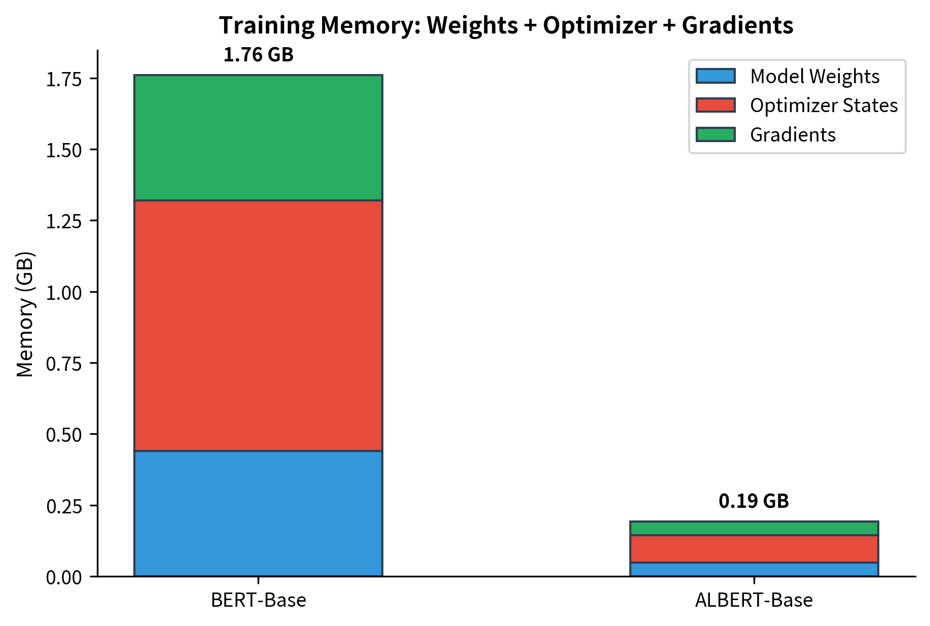
Memory and Speed Trade-offsLink Copied

Parameter sharing reduces memory for storing weights but doesn't reduce computation. ALBERT still performs the same number of matrix multiplications as BERT. The savings come from:

Model storage: The saved model is smaller.
Gradient memory: Only one set of layer gradients needed.
Optimizer states: Adam's momentum and variance buffers are smaller.

However, inference speed remains similar because the same operations execute.

In[40]:

Code

def compare_memory_requirements(bert_params, albert_params):
    """Compare memory requirements for training."""

    # Assumptions: FP32 (4 bytes), Adam optimizer (2x model for momentum/variance)
    bytes_per_param = 4

    bert_model_memory = bert_params * bytes_per_param / 1e9  # GB
    albert_model_memory = albert_params * bytes_per_param / 1e9

    # Adam optimizer states
    bert_optimizer_memory = 2 * bert_model_memory
    albert_optimizer_memory = 2 * albert_model_memory

    # Gradients (same as model)
    bert_gradient_memory = bert_model_memory
    albert_gradient_memory = albert_model_memory

    return {
        "bert": {
            "model": bert_model_memory,
            "optimizer": bert_optimizer_memory,
            "gradients": bert_gradient_memory,
            "total": bert_model_memory
            + bert_optimizer_memory
            + bert_gradient_memory,
        },
        "albert": {
            "model": albert_model_memory,
            "optimizer": albert_optimizer_memory,
            "gradients": albert_gradient_memory,
            "total": albert_model_memory
            + albert_optimizer_memory
            + albert_gradient_memory,
        },
    }

def compare_memory_requirements(bert_params, albert_params):
    """Compare memory requirements for training."""

    # Assumptions: FP32 (4 bytes), Adam optimizer (2x model for momentum/variance)
    bytes_per_param = 4

    bert_model_memory = bert_params * bytes_per_param / 1e9  # GB
    albert_model_memory = albert_params * bytes_per_param / 1e9

    # Adam optimizer states
    bert_optimizer_memory = 2 * bert_model_memory
    albert_optimizer_memory = 2 * albert_model_memory

    # Gradients (same as model)
    bert_gradient_memory = bert_model_memory
    albert_gradient_memory = albert_model_memory

    return {
        "bert": {
            "model": bert_model_memory,
            "optimizer": bert_optimizer_memory,
            "gradients": bert_gradient_memory,
            "total": bert_model_memory
            + bert_optimizer_memory
            + bert_gradient_memory,
        },
        "albert": {
            "model": albert_model_memory,
            "optimizer": albert_optimizer_memory,
            "gradients": albert_gradient_memory,
            "total": albert_model_memory
            + albert_optimizer_memory
            + albert_gradient_memory,
        },
    }

Out[41]:

Console

Training Memory Requirements (FP32, Adam optimizer):
--------------------------------------------------
Component               BERT-Base  ALBERT-Base
--------------------------------------------------
Model weights              0.44 GB       0.05 GB
Optimizer states           0.88 GB       0.10 GB
Gradients                  0.44 GB       0.05 GB
--------------------------------------------------
Total (weights only)       1.76 GB       0.19 GB

Note: Activation memory (batch, sequence length) is the same for both.

Out[42]:

Visualization

Stacked bar chart comparing memory requirements for BERT and ALBERT training components. — Training memory breakdown for BERT vs ALBERT. Parameter-related memory (weights, optimizer states, gradients) scales with model size. ALBERT's smaller parameter count dramatically reduces these components, though activation memory remains unchanged.

Performance BenchmarksLink Copied

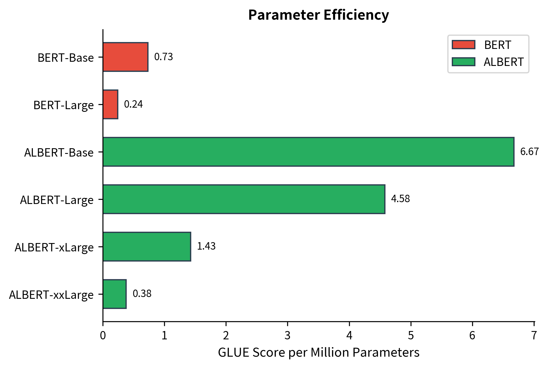
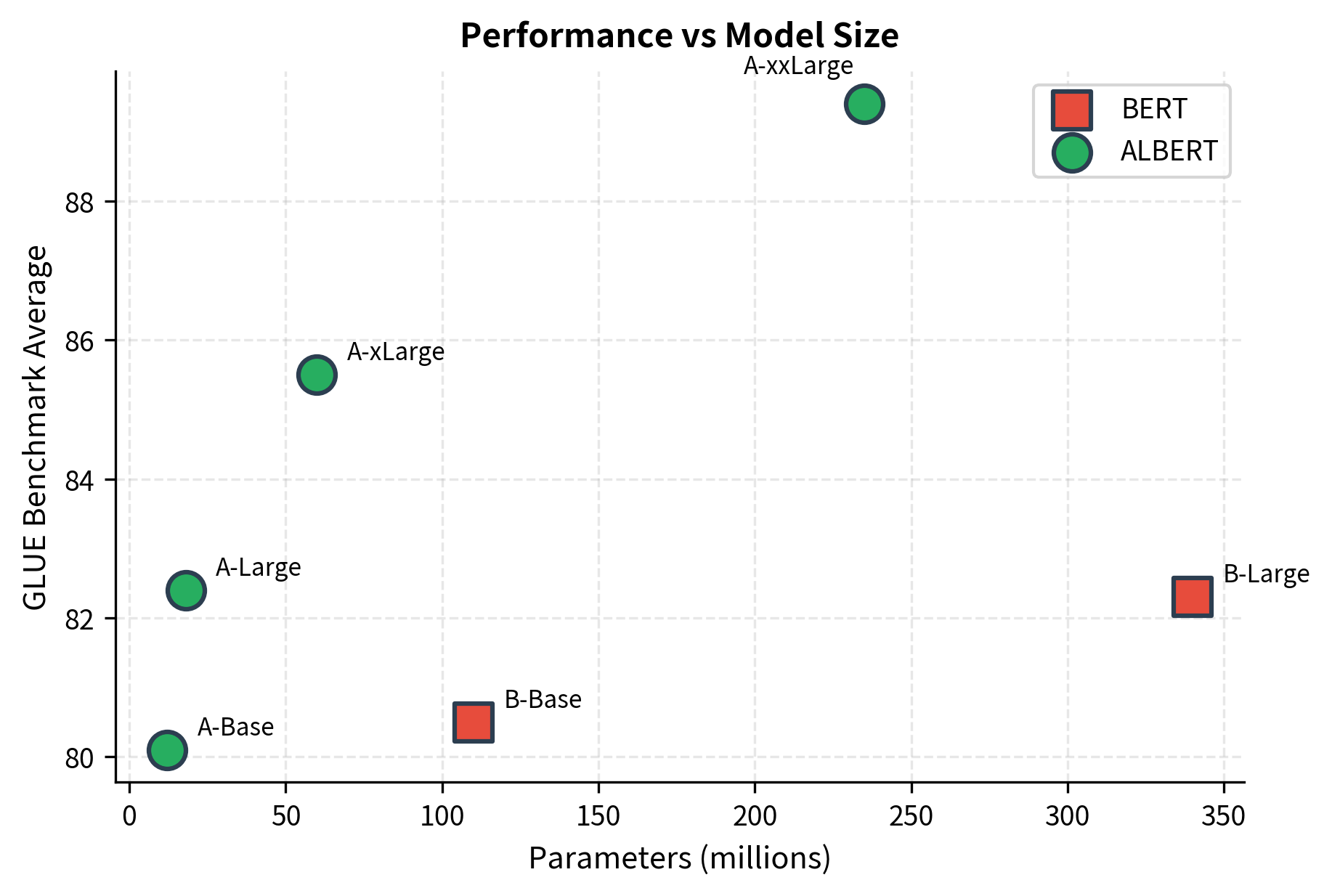
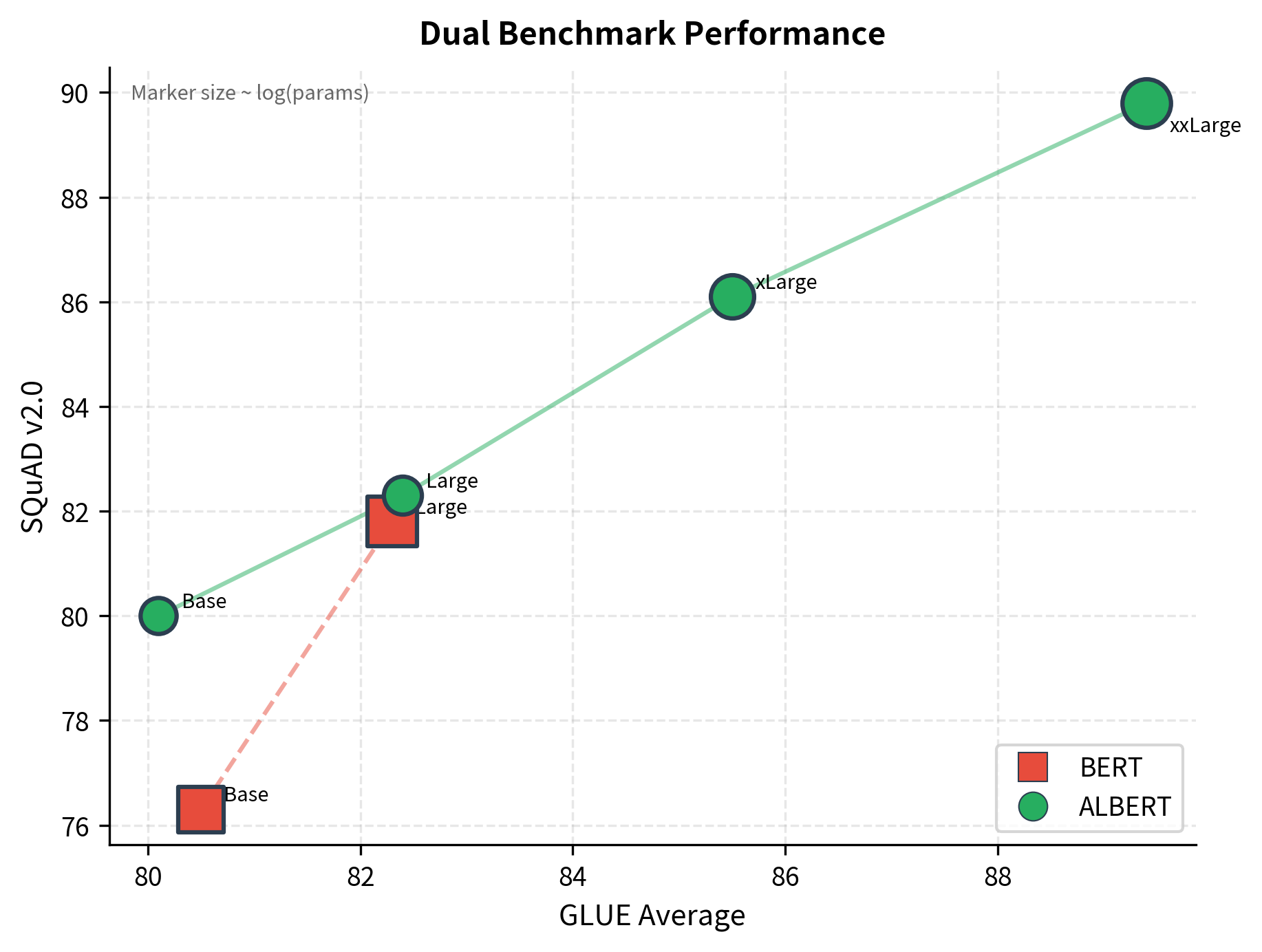
The ALBERT paper demonstrated that smaller models could match or exceed BERT's performance. On GLUE benchmark tasks, ALBERT-xxLarge achieved state-of-the-art results despite having fewer unique parameters than BERT-Large.

The key finding: representation quality depends more on model width and depth of computation than on parameter count. ALBERT's shared parameters still learn effective transformations when applied repeatedly.

In[43]:

Code

# Reported performance from the ALBERT paper (GLUE dev set average)
benchmark_results = {
    "BERT-Base": {"params": 110, "glue_avg": 80.5, "squad_v2": 76.3},
    "BERT-Large": {"params": 340, "glue_avg": 82.3, "squad_v2": 81.8},
    "ALBERT-Base": {"params": 12, "glue_avg": 80.1, "squad_v2": 80.0},
    "ALBERT-Large": {"params": 18, "glue_avg": 82.4, "squad_v2": 82.3},
    "ALBERT-xLarge": {"params": 60, "glue_avg": 85.5, "squad_v2": 86.1},
    "ALBERT-xxLarge": {"params": 235, "glue_avg": 89.4, "squad_v2": 89.8},
}

# Reported performance from the ALBERT paper (GLUE dev set average)
benchmark_results = {
    "BERT-Base": {"params": 110, "glue_avg": 80.5, "squad_v2": 76.3},
    "BERT-Large": {"params": 340, "glue_avg": 82.3, "squad_v2": 81.8},
    "ALBERT-Base": {"params": 12, "glue_avg": 80.1, "squad_v2": 80.0},
    "ALBERT-Large": {"params": 18, "glue_avg": 82.4, "squad_v2": 82.3},
    "ALBERT-xLarge": {"params": 60, "glue_avg": 85.5, "squad_v2": 86.1},
    "ALBERT-xxLarge": {"params": 235, "glue_avg": 89.4, "squad_v2": 89.8},
}

Out[44]:

Console

Model Performance Comparison:
-----------------------------------------------------------------
Model              Parameters   GLUE Avg     SQuAD v2.0  
-----------------------------------------------------------------
BERT-Base               110M       80.5         76.3
BERT-Large              340M       82.3         81.8
ALBERT-Base              12M       80.1         80.0
ALBERT-Large             18M       82.4         82.3
ALBERT-xLarge            60M       85.5         86.1
ALBERT-xxLarge          235M       89.4         89.8

A useful metric for comparing models is parameter efficiency, which measures performance per million parameters. This reveals which architectures extract the most value from their parameters:

Out[45]:

Visualization

Bar chart showing GLUE score per million parameters for each model. — Parameter efficiency (GLUE score per million parameters) across models. ALBERT-Base achieves the highest efficiency, extracting 6.7 GLUE points per million parameters compared to BERT-Base's 0.73. Even ALBERT-xxLarge, while less efficient than smaller ALBERTs, still outperforms BERT models in efficiency.

Out[46]:

Visualization

Scatter plot showing GLUE benchmark scores vs parameter count for various BERT and ALBERT models. — Performance vs parameters for BERT and ALBERT models. ALBERT achieves better performance-to-parameter ratios, with ALBERT-xLarge matching BERT-Large performance at ~6x fewer parameters. ALBERT-xxLarge sets new records despite using shared parameters.

We can also compare performance across both GLUE and SQuAD benchmarks simultaneously:

Out[47]:

Visualization

Scatter plot with GLUE score on x-axis and SQuAD score on y-axis, showing model performance trajectories. — BERT vs ALBERT performance on GLUE and SQuAD v2.0 benchmarks. ALBERT models consistently outperform BERT models with similar parameter counts. The shaded region connects same-family models, showing ALBERT's steeper performance scaling.

When to Use ALBERTLink Copied

ALBERT shines in specific scenarios:

Memory-constrained environments: When GPU memory limits model size, ALBERT's smaller parameter count allows training larger effective models.
Transfer learning: ALBERT's pretrained weights are smaller to download and store.
Ensemble models: Multiple ALBERT models fit where one BERT might not.

However, ALBERT is not always the best choice:

Inference latency: Same computational cost as BERT means similar inference time.
Simple tasks: For easy tasks, smaller unique-parameter models might suffice.
Maximum performance: At extreme scales, unique parameters can still outperform shared ones.

The following table summarizes these trade-offs:

BERT vs ALBERT comparison. ALBERT trades unique parameters for memory efficiency while maintaining computational depth.

Aspect	BERT	ALBERT
Parameters	110M (Base), 340M (Large)	12M (Base), 18M (Large)
Training memory	Higher	Lower
Inference speed	Same	Same
Model file size	Larger	Smaller
Layer expressiveness	Unique per layer	Shared across layers
Embedding approach	Direct (vocab to hidden)	Factorized (vocab to small, then to hidden)

Limitations and ImpactLink Copied

ALBERT's innovations come with important caveats that affect practical deployment.

The shared-parameter design creates a fundamental tension. While repeating the same transformation refines representations, it also limits what each pass can do. Unique layers can specialize: early layers might focus on syntax while later layers capture semantics. Shared layers must compromise, learning a transformation that works reasonably well at every depth. For some tasks, this constraint hurts. The original paper showed that very deep ALBERT models sometimes underperform shallower ones because the repeated transformation eventually stops improving representations.

Inference speed remains unchanged despite the smaller parameter count. ALBERT still multiplies inputs by the same-sized weight matrices the same number of times. Memory savings during inference are minimal because activation memory dominates over weight memory. For production systems where latency matters more than storage, ALBERT offers limited advantage over BERT.

The factorized embedding dimension also presents trade-offs. Setting $E = 128$ works well empirically, but the optimal value depends on vocabulary size and downstream tasks. Too small an embedding dimension compresses token information too aggressively. The projection layer can only recover what was preserved in the bottleneck.

Despite these limitations, ALBERT's impact on the field was substantial. It demonstrated that parameter efficiency and model quality are not fundamentally opposed. The techniques it introduced, factorized embeddings and cross-layer sharing, appeared in subsequent architectures. Perhaps more importantly, ALBERT challenged the assumption that progress requires ever-larger models. By showing that 12 million parameters could match 110 million, it encouraged research into what models actually need versus what they happen to have.

Key ParametersLink Copied

When configuring an ALBERT model, these parameters most significantly affect performance and efficiency:

embedding_dim: The intermediate embedding dimension before projection to hidden size. ALBERT uses 128 for all model sizes. Smaller values save more parameters but may compress token information too aggressively. Values between 64-256 are reasonable starting points.
hidden_dim: The dimension of representations flowing through transformer layers. Larger values increase model capacity but also increase compute cost per layer. ALBERT scales this dimension (768 to 4096) rather than adding unique layers.
num_layers: The number of times the shared layer is applied. More applications allow more iterative refinement but increase compute time. With shared parameters, adding layers costs nothing in memory for weights, only activation memory.
num_heads: The number of attention heads in multi-head attention. Must divide hidden_dim evenly. More heads allow the model to attend to different aspects of the input simultaneously but increase the attention computation overhead.
intermediate_dim: The dimension of the feed-forward network's hidden layer, typically 4x the hidden_dim. Larger values increase the network's capacity to transform representations.
dropout: Regularization applied during training. Standard values range from 0.0 to 0.1. Higher dropout can help prevent overfitting but may slow learning.
max_position: Maximum sequence length the model can handle. ALBERT uses 512 like BERT. Longer sequences require more memory for attention computation, which scales quadratically with length.

SummaryLink Copied

ALBERT introduced two key innovations for building more efficient transformers:

Factorized embeddings decompose the large embedding matrix into two smaller matrices. Instead of directly mapping vocabulary tokens to hidden-dimension vectors (requiring $V \times H$ parameters), ALBERT first maps to a smaller embedding space ( $V \times E$ parameters) then projects up ( $E \times H$ parameters). When the embedding dimension $E$ is much smaller than the hidden dimension $H$ , this reduces embedding parameters by up to 80%.
Cross-layer parameter sharing uses a single set of transformer weights applied repeatedly, cutting layer parameters by a factor equal to the number of layers.
Sentence Order Prediction replaces the easier NSP task with order detection, requiring genuine discourse understanding rather than topic matching.
Iterative refinement emerges from shared parameters, as the model applies the same transformation multiple times to progressively refine representations.
Memory benefits during training come from smaller optimizer states and gradient buffers, though inference speed matches BERT due to identical computation.
Performance parity demonstrated that model quality depends more on computational depth and width than on unique parameter count, with ALBERT-xxLarge achieving state-of-the-art results.

ALBERT showed that careful architecture design could dramatically reduce model size without sacrificing performance, influencing subsequent work on efficient transformers.

QuizLink Copied

Ready to test your understanding? Take this quick quiz to reinforce what you've learned about ALBERT's parameter-efficient architecture.

Loading component...

Track your reading progress

Sign in to mark chapters as read and track your learning journey

Sign in →

Comments

Back to Language AI Handbook

Reference

BIBTEXAcademic

@misc{albertparameterefficientbertwithfactorizedembeddings, author = {Michael Brenndoerfer}, title = {ALBERT: Parameter-Efficient BERT with Factorized Embeddings}, year = {2025}, url = {https://mbrenndoerfer.com/writing/albert-parameter-efficient-bert-factorized-embeddings}, organization = {mbrenndoerfer.com}, note = {Accessed: 2025-12-19} }

APAAcademic

Michael Brenndoerfer (2025). ALBERT: Parameter-Efficient BERT with Factorized Embeddings. Retrieved from https://mbrenndoerfer.com/writing/albert-parameter-efficient-bert-factorized-embeddings

MLAAcademic

Michael Brenndoerfer. "ALBERT: Parameter-Efficient BERT with Factorized Embeddings." 2025. Web. 12/19/2025. <https://mbrenndoerfer.com/writing/albert-parameter-efficient-bert-factorized-embeddings>.

CHICAGOAcademic

Michael Brenndoerfer. "ALBERT: Parameter-Efficient BERT with Factorized Embeddings." Accessed 12/19/2025. https://mbrenndoerfer.com/writing/albert-parameter-efficient-bert-factorized-embeddings.

HARVARDAcademic

Michael Brenndoerfer (2025) 'ALBERT: Parameter-Efficient BERT with Factorized Embeddings'. Available at: https://mbrenndoerfer.com/writing/albert-parameter-efficient-bert-factorized-embeddings (Accessed: 12/19/2025).

SimpleBasic

Michael Brenndoerfer (2025). ALBERT: Parameter-Efficient BERT with Factorized Embeddings. https://mbrenndoerfer.com/writing/albert-parameter-efficient-bert-factorized-embeddings

Direct link:

https://mbrenndoerfer.com/writing/albert-parameter-efficient-bert-factorized-embeddings

About the author: Michael Brenndoerfer

All opinions expressed here are my own and do not reflect the views of my employer.

Michael currently works as an Associate Director of Data Science at EQT Partners in Singapore, leading AI and data initiatives across private capital investments.

With over a decade of experience spanning private equity, management consulting, and software engineering, he specializes in building and scaling analytics capabilities from the ground up. He has published research in leading AI conferences and holds expertise in machine learning, natural language processing, and value creation through data.

View Full Resume Publications Contact Books

ALBERT: Parameter-Efficient BERT with Factorized Embeddings

ALBERTLink Copied

The Parameter ProblemLink Copied

Factorized Embedding ParameterizationLink Copied

Why Factorization WorksLink Copied

Iterative RefinementLink Copied

Sentence Order PredictionLink Copied

Implementing a Complete ALBERT ModelLink Copied

ALBERT Model ConfigurationsLink Copied

Training ALBERTLink Copied

Memory and Speed Trade-offsLink Copied

Performance BenchmarksLink Copied

When to Use ALBERTLink Copied

Limitations and ImpactLink Copied

Key ParametersLink Copied

SummaryLink Copied

QuizLink Copied

Comments

Reference

About the author: Michael Brenndoerfer

Related Content

ELECTRA: Efficient Pre-training with Replaced Token Detection

BERT Fine-tuning: Classification, NER & Question Answering

DeBERTa: Disentangled Attention and Enhanced Mask Decoding

Stay updated

ALBERT: Parameter-Efficient BERT with Factorized Embeddings

ALBERTLink Copied

The Parameter ProblemLink Copied

Factorized Embedding ParameterizationLink Copied

Why Factorization WorksLink Copied

Cross-Layer Parameter SharingLink Copied

Different Sharing StrategiesLink Copied

Iterative RefinementLink Copied

Sentence Order PredictionLink Copied

Implementing a Complete ALBERT ModelLink Copied

ALBERT Model ConfigurationsLink Copied

Training ALBERTLink Copied

Memory and Speed Trade-offsLink Copied

Performance BenchmarksLink Copied

When to Use ALBERTLink Copied

Limitations and ImpactLink Copied

Key ParametersLink Copied

SummaryLink Copied

QuizLink Copied

Comments

Reference

About the author: Michael Brenndoerfer

Related Content

ELECTRA: Efficient Pre-training with Replaced Token Detection

BERT Fine-tuning: Classification, NER & Question Answering

DeBERTa: Disentangled Attention and Enhanced Mask Decoding

Stay updated