Quadratic Attention Bottleneck: Why Transformers Struggle with Long Sequences

Transformers have revolutionized natural language processing, powering everything from chatbots to code assistants. At the heart of their success lies self-attention, a mechanism that allows every token to directly interact with every other token. This all-pairs computation is both the transformer's greatest strength and its Achilles' heel. As sequence length grows, the computational and memory demands explode quadratically, creating a fundamental barrier to processing long documents, extended conversations, and book-length texts.

In this chapter, we analyze why this quadratic bottleneck exists, quantify its impact on real systems, and visualize how quickly resources become exhausted. Understanding this limitation sets the stage for the efficient attention variants covered in subsequent chapters.

Self-attention computes relationships between every pair of tokens in a sequence. For a sequence of $n$ tokens, this means $n^2$ pairwise interactions. The complete attention formula is:

where:

• $Q \in \mathbb{R}^{n \times d_k}$: query matrix with one row per token
• $K \in \mathbb{R}^{n \times d_k}$: key matrix with one row per token
• $V \in \mathbb{R}^{n \times d_v}$: value matrix containing information to aggregate
• $d_k$: dimension of queries and keys
• $n$: sequence length

The critical operation is $QK^T$, which produces an $n \times n$ attention score matrix. Every element $(i, j)$ in this matrix represents how much token $i$ should attend to token $j$. Computing all $n^2$ entries is what gives attention its power: any token can directly influence any other, regardless of distance. But this same property creates the quadratic scaling problem.

Consider the contrast with sequential processing. In a recurrent neural network, information from token 1 must propagate through tokens 2, 3, 4, and so on to reach token 100. In attention, token 1 directly connects to token 100 in a single step. This short path length is why transformers excel at capturing long-range dependencies. However, the price is computing all pairwise interactions up front.

The "Growth Factor" column reveals the quadratic pattern: doubling the sequence length quadruples the number of interactions. At 128 tokens, we compute roughly 16,000 pairs. At 4096 tokens, this explodes to over 16 million pairs. The 4x growth for each 2x increase in sequence length is the signature of $O(n^2)$ complexity.

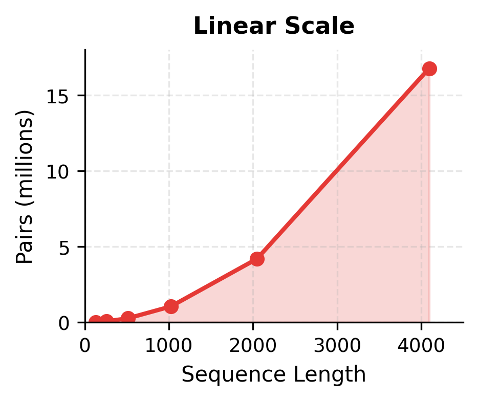
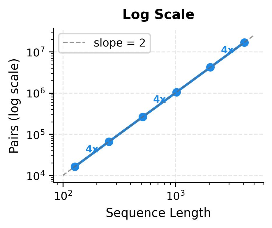
The first panel shows the raw explosion in pair count, rising from near zero at short sequences to over 16 million at 4096 tokens. The second panel, using logarithmic scales on both axes, reveals the underlying structure: a straight line with slope 2, confirming the $n^2$ relationship. Each doubling of sequence length produces exactly a 4x increase in pairs, marked along the curve.

The attention score matrix consumes memory proportional to $n^2$. Each attention head computes its own $n \times n$ matrix of attention weights, and these matrices must be stored during both forward and backward passes. For a model with $h$ attention heads, the total memory required for attention matrices in a single layer is:

where:

• $M_{\text{attn}}$: memory in bytes for attention matrices
• $h$: number of attention heads (each head computes an independent attention pattern)
• $n$: sequence length (number of tokens)
• $n^2$: the number of entries in each attention matrix (one score per query-key pair)
• $b$: bytes per element (4 for fp32, 2 for fp16/bf16)

The formula reflects a simple structure: $h$ heads times $n^2$ entries per head times $b$ bytes per entry. The $n^2$ term is the source of quadratic scaling.

Worked Example: With 12 attention heads, fp16 precision, and a sequence length of 8192 tokens, the attention matrices for a single layer consume:

For a 12-layer transformer, this becomes approximately 19 GB just for attention matrices, before accounting for model weights, activations, or gradients.

The memory requirements reveal why long-context models are challenging. A GPT-2 Small model at 512 tokens uses only about 0.07 GB for attention matrices. At 8192 tokens, this grows to nearly 18 GB. At 32K tokens, a modest 12-layer model requires over 280 GB just for attention, exceeding the memory of any single GPU. Larger models with more heads and layers face even steeper memory walls.

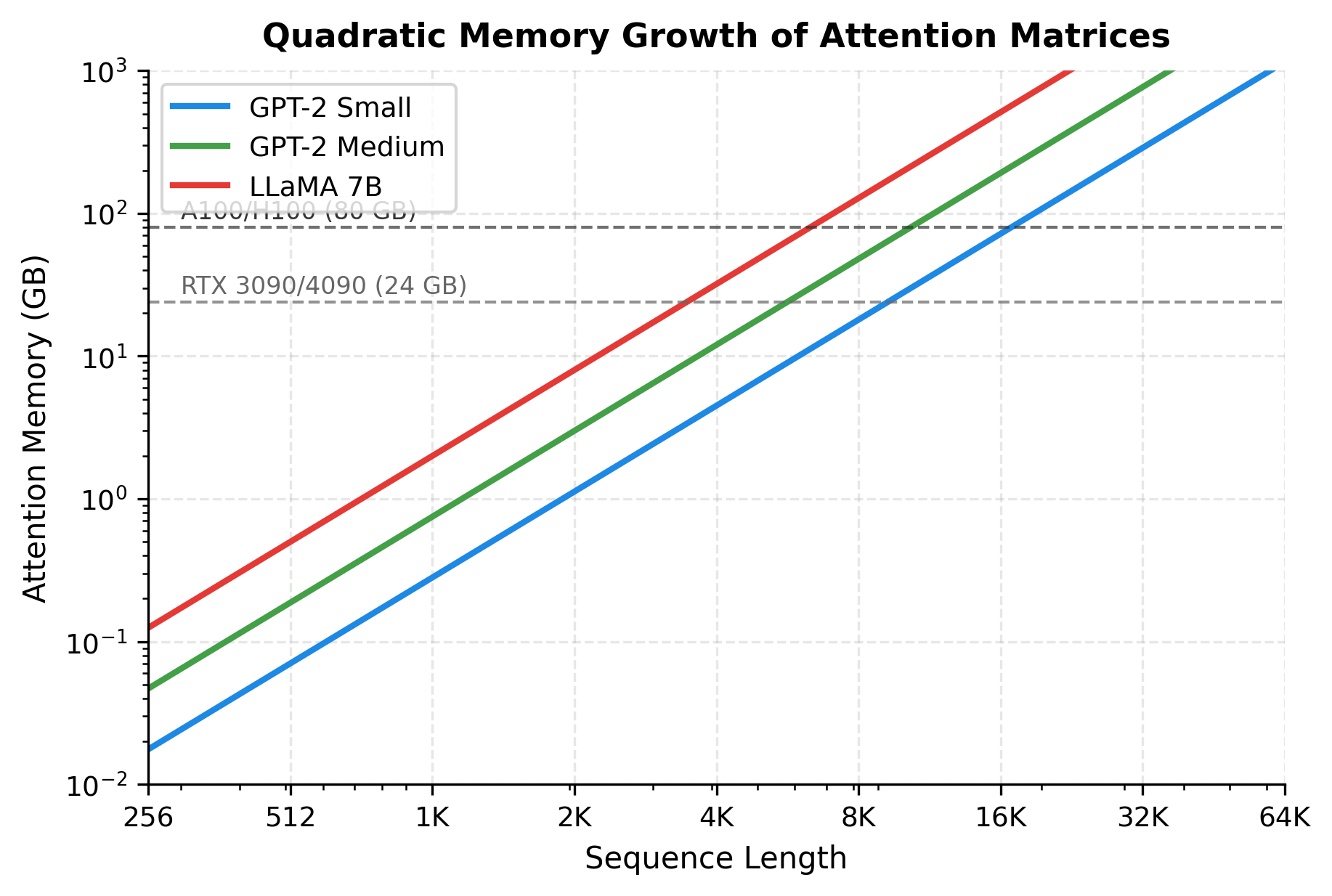
The plot shows that even the smallest model configuration exceeds a 24 GB GPU around 16K tokens, and an 80 GB GPU around 32K tokens. Larger models hit these limits much sooner. This memory wall is often the first constraint encountered when extending context length.

We've seen that attention requires storing an $n \times n$ matrix of weights. But how much computation does it take to produce those weights and use them? Understanding the computational cost helps us predict training times, estimate inference latency, and appreciate why efficient attention variants are so valuable.

The answer turns out to be $O(n^2 d)$ floating-point operations per attention layer. To see where this comes from, let's trace through exactly what happens when attention runs.

Before diving into the math, consider what attention needs to accomplish for each token in the sequence:

1. Compare this token to every other token to determine relevance scores
2. Normalize those scores into a probability distribution
3. Blend information from all tokens according to those probabilities

For a sequence of $n$ tokens, step 1 alone requires $n$ comparisons per token, and we have $n$ tokens, giving us $n \times n = n^2$ comparisons. This is the fundamental source of quadratic scaling: the all-pairs comparison cannot be avoided in standard attention.

Now let's quantify each step precisely.

The first operation computes how strongly each query should attend to each key. Mathematically, this is the matrix multiplication $QK^T$, where $Q$ contains all query vectors (one per token) and $K$ contains all key vectors.

When we multiply a matrix of shape $(n \times d_k)$ by a transposed matrix of shape $(d_k \times n)$, we get an $(n \times n)$ output. Each entry in this output matrix is a dot product between one query and one key, requiring $d_k$ multiplications and $d_k - 1$ additions. With $n^2$ such entries, the total operation count is:

where:

• $n^2$: the number of query-key pairs (one score per pair)
• $d_k$: the dimension of each query and key vector
• $2$: accounts for both multiplications and additions in each dot product

The $n^2$ appears because every token must be compared against every other token. There's no shortcut here: we don't know which pairs will have high attention until we compute all the scores.

Raw dot products can be any real number, positive or negative. To use them as weights in a weighted average, we need to convert each row of scores into a probability distribution that sums to 1. The softmax function accomplishes this:

where $s_i$ is the $i$-th attention score in a row, and the sum runs over all $n$ scores in that row.

For each of the $n$ rows in the attention matrix, softmax requires:

• Exponentiating $n$ scores
• Summing those $n$ exponentials
• Dividing each of the $n$ exponentials by the sum

This contributes roughly $5n$ operations per row (exponentiate, sum, divide, with some overhead). With $n$ rows:

While still quadratic in $n$, the softmax cost lacks the $d_k$ factor, making it smaller than score computation when $d_k$ is large. For typical transformers where $d_k = 64$ to $128$, softmax contributes less than 10% of the total attention FLOPs.

The final step uses the normalized attention weights to compute a weighted combination of value vectors. Each token's output is a blend of all tokens' values, weighted by attention:

This is another matrix multiplication: the $(n \times n)$ attention weights multiplied by the $(n \times d_v)$ value matrix produces an $(n \times d_v)$ output. Each of the $n \times d_v$ output elements requires summing across $n$ weighted values:

This matches the cost of score computation. We've encountered two expensive $O(n^2 d)$ operations, and they dominate the total cost.

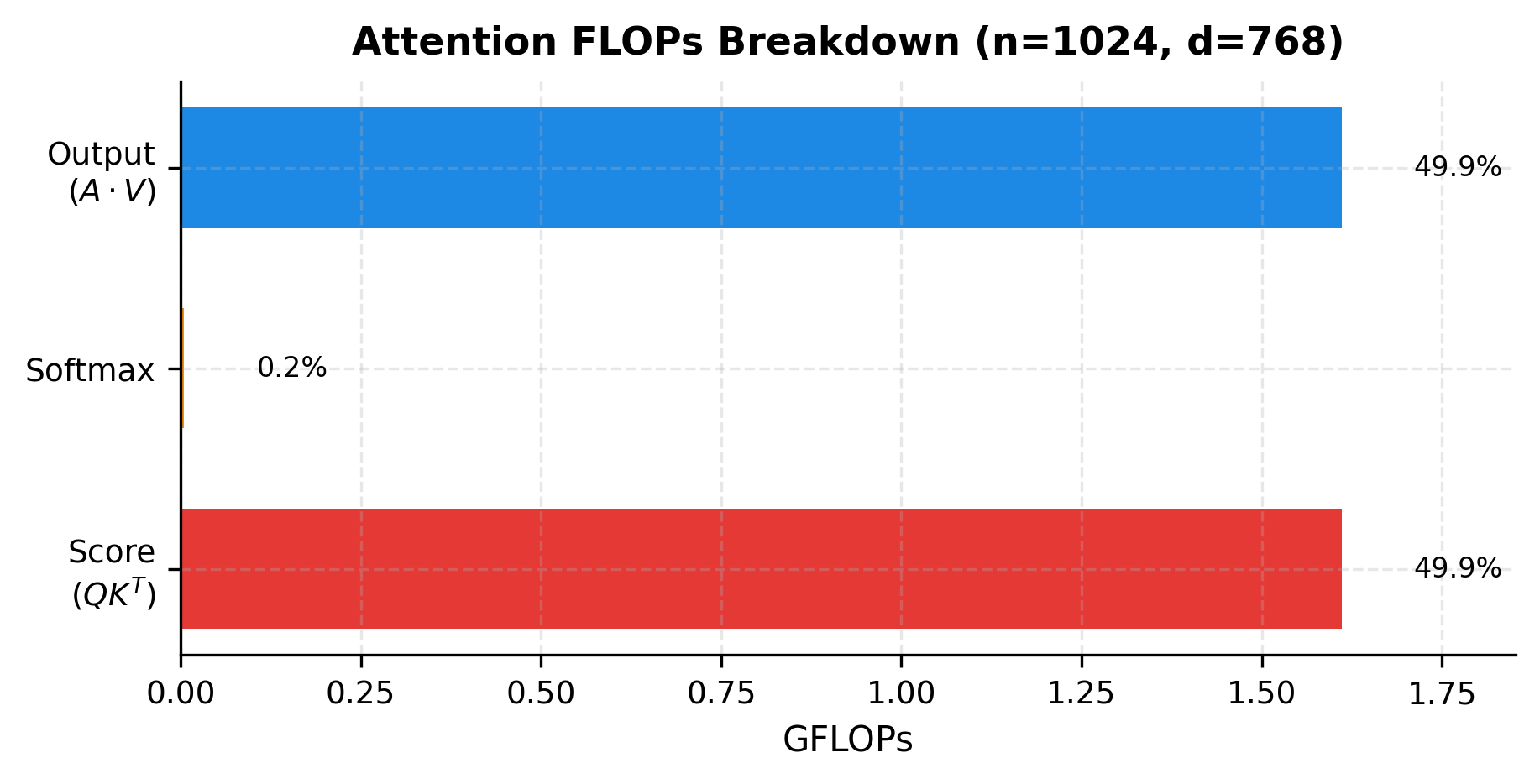
The visualization confirms our analysis: score computation and output computation each consume roughly half the total FLOPs (about 49.8% each), while softmax contributes less than 0.4%. The two matrix multiplications involving the $n \times n$ attention matrix dominate entirely.

Combining all three stages, the total computational cost of self-attention is:

where:

• $n$: sequence length (number of tokens)
• $d_k$: dimension of query and key vectors (typically $d/h$)
• $d_v$: dimension of value vectors (typically equal to $d_k$)
• $d$: model dimension (the full embedding size before splitting into heads)
• $h$: number of attention heads

The simplification to $O(n^2 d)$ holds because $d_k$ and $d_v$ are both proportional to $d$. In standard transformers, each head operates on $d/h$ dimensions, and since we sum across all heads, the total work scales with the full model dimension.

The formula reveals an asymmetry in how the two factors affect complexity:

• Doubling $n$ quadruples the computation because $n$ appears squared
• Doubling $d$ only doubles the computation because $d$ appears linearly

This asymmetry has profound implications. For a model with $d = 768$ processing $n = 4096$ tokens, the $n^2 = 16{,}777{,}216$ factor dwarfs the $d = 768$ factor by a ratio of over 20,000 to 1. The quadratic term completely dominates, which is why sequence length is the bottleneck rather than model size.

Let's make this concrete by computing the actual FLOPs for a GPT-2 style model with $d = 768$:

The numbers tell the story of quadratic growth. At 512 tokens, a single attention layer performs about 1.6 billion operations, which modern GPUs handle in microseconds. At 2048 tokens (4x longer), the count grows to roughly 26 billion operations (16x more, confirming the quadratic relationship). By 32,768 tokens, we're approaching 7 trillion operations per layer.

For a complete transformer, multiply these numbers by the layer count. A 12-layer GPT-2 at 4096 tokens performs over 1.2 trillion attention operations. During training, backpropagation roughly triples this cost (forward pass, backward for computing gradients, backward for applying updates). The computational demands compound rapidly, and attention becomes the dominant bottleneck for long sequences.

The $n \times n$ attention matrix lies at the center of the bottleneck. Visualizing its structure helps build intuition for why it's both powerful and expensive.

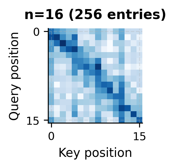
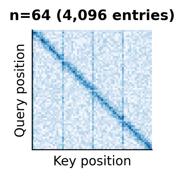
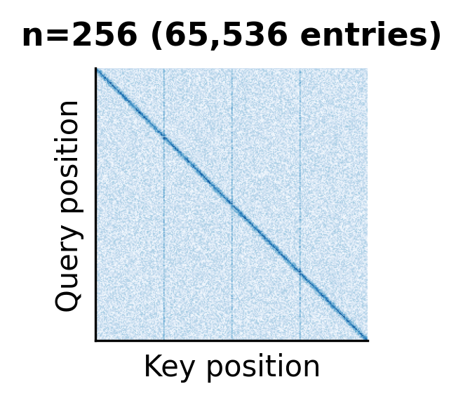
As the sequence length grows, the attention matrix balloons in size. At $n=16$, the matrix is compact and easy to visualize. At $n=256$, individual cells become indistinguishable. At $n=8192$ (a common context length for modern LLMs), the matrix would contain over 67 million entries, impossible to render at a reasonable resolution.

The structured patterns visible in these matrices hint at why sparse attention methods work. Much of the attention mass concentrates on the diagonal (local context), certain global tokens, and specific positions. The full $n^2$ matrix contains much redundancy that efficient methods can exploit.

Given the quadratic scaling, what are the practical limits for standard attention? The answer depends on hardware constraints and whether you're training or doing inference.

These estimates reveal a stark reality. Even on an 80 GB GPU, training a standard transformer is limited to roughly 16K-23K tokens before memory runs out. Inference allows longer sequences since gradients aren't stored, but even then, sequences beyond 50K tokens become challenging. Production models that claim 100K+ context windows use specialized techniques covered in later chapters.

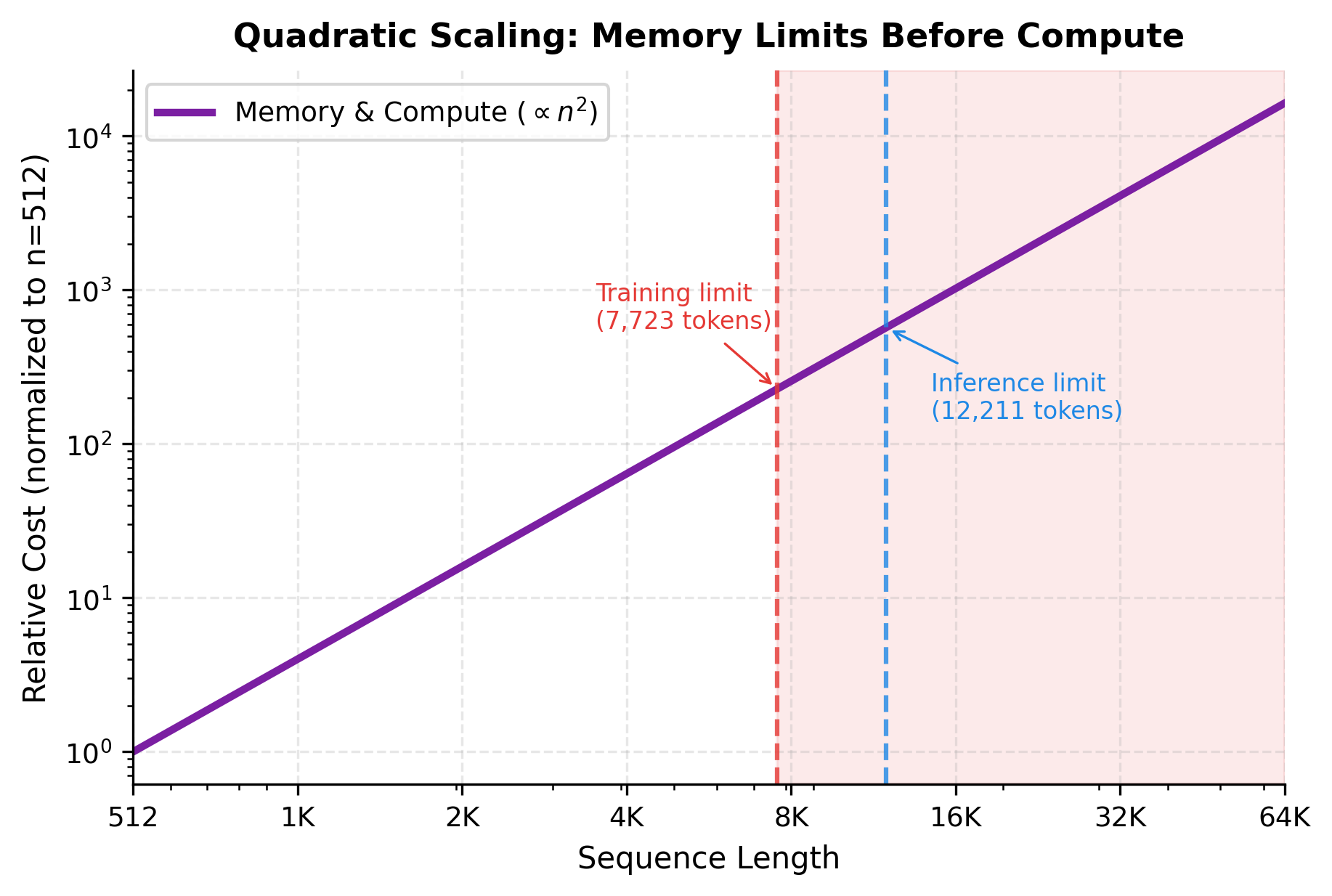
The shaded region represents sequence lengths that exceed GPU memory for training. While compute could theoretically handle longer sequences given enough time, memory is a hard constraint that cannot be overcome without specialized techniques. This asymmetry explains why memory-efficient attention methods like FlashAttention have had such impact: they shift the memory limit rightward without changing the compute requirements.

To fully appreciate the quadratic bottleneck, we can visualize how attention costs compare to other transformer components as sequence length grows.

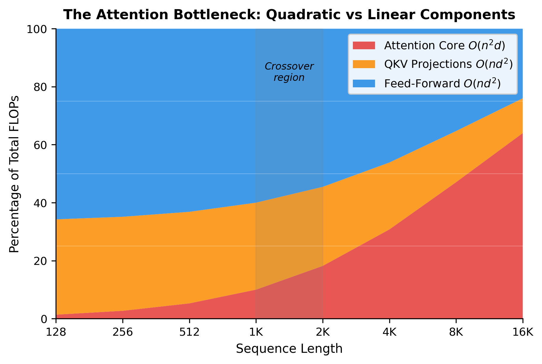
At short sequence lengths (128-256 tokens), the feed-forward network and projections dominate, and attention contributes less than 10% of total computation. As sequences grow, the quadratic term takes over. By 4K tokens, attention accounts for nearly half of all operations. At 16K tokens and beyond, attention consumes the vast majority of compute budget, squeezing out everything else.

This is the attention bottleneck in visual form. Optimizing transformers for long sequences means addressing the red region in this chart.

The quadratic bottleneck motivates several lines of research, each tackling the problem from a different angle:

Each approach involves trade-offs. Sparse attention sacrifices some global interactions. Linear attention may lose expressiveness on certain tasks. Memory-efficient methods require careful implementation and may have higher constant factors. The following chapters explore each in detail.

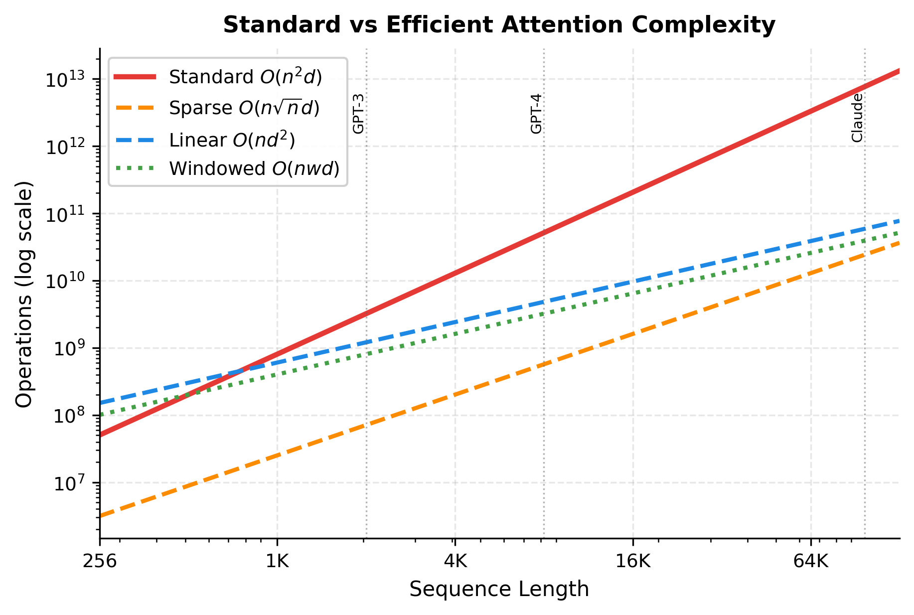
The gap between standard attention (red) and efficient variants grows dramatically at long sequences. At 64K tokens, sparse attention requires roughly 250x fewer operations than standard attention. This difference is what enables modern long-context models to process book-length documents.

The quadratic attention bottleneck is a fundamental constraint that shapes transformer design and deployment. In this chapter, we quantified the $O(n^2)$ scaling in both memory and compute, visualized how attention costs grow to dominate transformer computation, and previewed the efficient attention variants that address this limitation.

Key takeaways:

• Quadratic memory: Storing attention matrices requires $O(h \cdot n^2)$ memory, where $h$ is the number of attention heads and $n$ is the sequence length. This often becomes the first constraint hit when extending context length.

• Quadratic compute: The attention core requires $O(n^2 d)$ operations, where $n$ is sequence length and $d$ is model dimension. Doubling sequence length quadruples attention computation.

• The crossover point: At short sequences, attention is a minor cost. At long sequences (roughly 1K-4K tokens for typical models), attention becomes the dominant expense.

• Practical limits: Standard attention on current GPUs is limited to roughly 16K-32K tokens for training and 50K-100K tokens for inference, depending on model size and hardware.

• Motivation for efficiency: The quadratic bottleneck drives research into sparse attention, linear attention, and memory-efficient implementations, each trading different aspects to break the $O(n^2)$ barrier.

Understanding this bottleneck is essential for working with long-context models and for appreciating why the efficient attention techniques covered in the following chapters are so important. The $n^2$ wall is real, but it can be scaled with the right approaches.

When analyzing attention complexity or estimating resource requirements, these parameters directly determine memory and compute costs:

• n (sequence length): The number of tokens in the input. This is the most critical parameter since both memory and compute scale with $n^2$. Typical values range from 512 (early BERT) to 128K+ (modern long-context models).

• d (model dimension): The embedding dimension of the model. Common values include 768 (GPT-2 Small), 4096 (LLaMA 7B), and 8192 (larger models). Complexity scales linearly with $d$, making it less impactful than sequence length.

• h (number of heads): The number of parallel attention heads. Each head stores an independent $n \times n$ attention matrix, so memory scales linearly with $h$. Typical values range from 12 to 128.

• L (number of layers): The depth of the transformer. Memory for attention matrices scales linearly with layer count. A 24-layer model uses twice the attention memory of a 12-layer model.

• dtype_bytes: Precision of floating-point representation. Using fp16 (2 bytes) instead of fp32 (4 bytes) halves memory requirements and often doubles throughput on modern GPUs.

• overhead_factor: When estimating maximum sequence length, this represents the fraction of GPU memory available for attention matrices after accounting for model weights, activations, and gradients. Typical values are 0.5 for inference and 0.2 for training.

Ready to test your understanding? Take this quick quiz to reinforce what you've learned about the quadratic attention bottleneck.