Context Length Challenges: Memory, Position Encoding & Long-Range Dependencies

Transformers have conquered natural language processing, but they harbor a fundamental limitation: fixed context windows. A model trained on 2048 tokens cannot simply process 8192 tokens at inference time. This constraint affects everything from document summarization to multi-turn conversations, where earlier context often matters most.

The challenge isn't just about feeding more tokens into the model. It encompasses memory explosion from quadratic attention, position encodings that break beyond training lengths, the difficulty of learning dependencies across thousands of tokens, and the puzzle of evaluating whether models actually use long-range information. In this chapter, we systematically examine each of these barriers. Understanding them is essential before exploring the solutions covered in subsequent chapters.

Every transformer is trained on sequences of a fixed maximum length. GPT-2 used 1024 tokens. BERT used 512. Early GPT-3 models trained on 2048 tokens. These aren't arbitrary choices but rather pragmatic compromises between model capability and computational cost.

The training length fundamentally shapes what the model learns. A model trained on 512-token sequences has never seen how pronouns resolve across 1000 tokens or how conclusions connect to distant premises. These long-range patterns simply aren't in the training data.

The jump from 2K to 200K+ tokens represents a 100x increase in just a few years. This explosion in context length didn't come for free. Each extension required novel techniques for position encoding, memory efficiency, and training methodology.

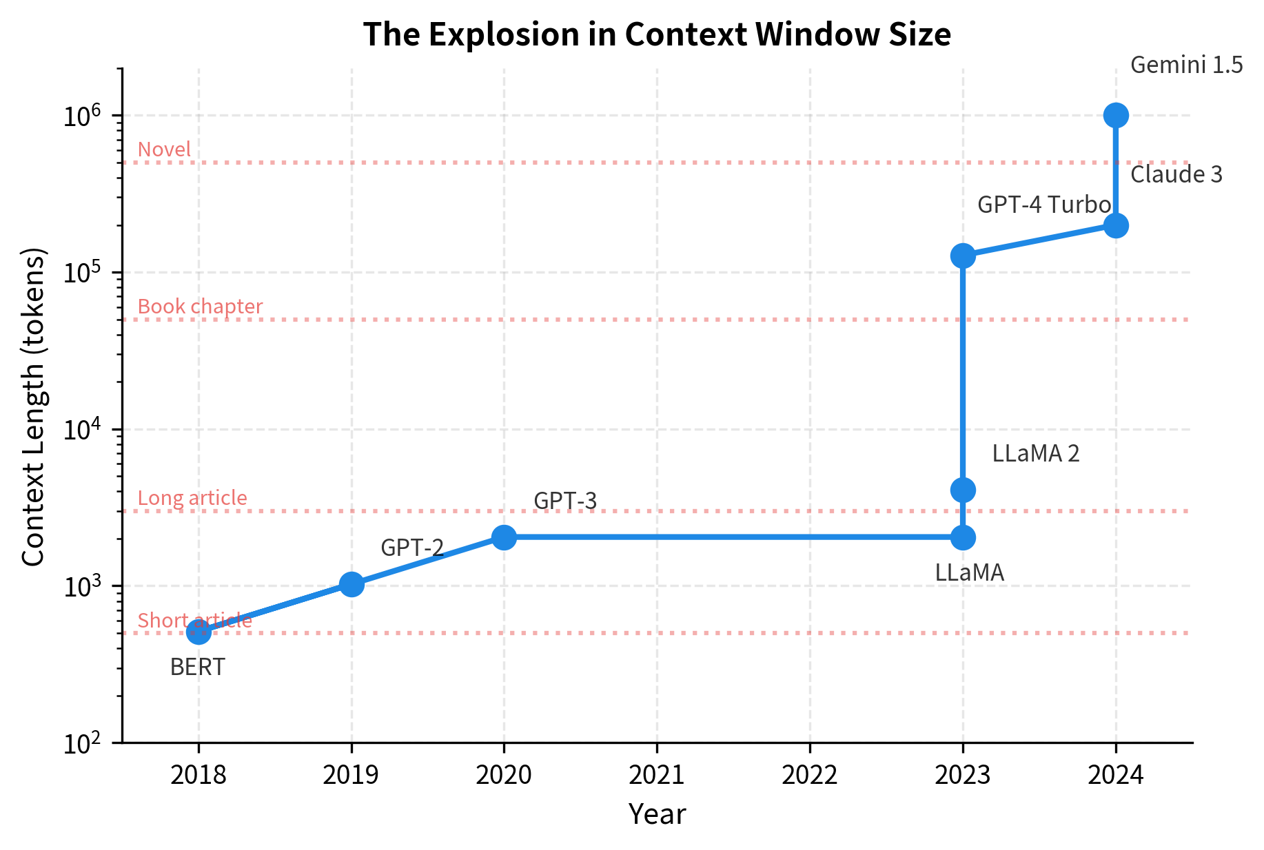
The progression reveals a pattern. Until 2023, context lengths grew modestly, doubling every few years. Then came a breakthrough. Models jumped from 4K to 100K+ tokens in a single generation. This wasn't just better hardware. It required fundamental advances in how position information is encoded and how attention is computed.

The obvious question: why didn't earlier models simply train on longer sequences? The answer involves multiple compounding constraints.

Memory scales quadratically. We explored this in detail in the previous chapter on the quadratic attention bottleneck. For a 4K token sequence, attention matrices alone consume 16x more memory than for 1K tokens. Training on 32K tokens with naive attention would require 1024x more attention memory than training on 1K tokens.

Compute scales quadratically too. Even if memory were free, the computational cost of training explodes. A batch of 32K-token sequences requires the same attention compute as 1024 batches of 1K-token sequences, holding total tokens constant.

Long documents are rare. Most training data consists of short documents. Web pages average a few thousand tokens. Training a model to handle 100K tokens requires curating datasets with genuinely long documents, which are harder to find and more expensive to process.

Gradients become unstable. Backpropagating through very long sequences compounds numerical errors. Without careful normalization and training tricks, models can fail to learn anything useful from long sequences.

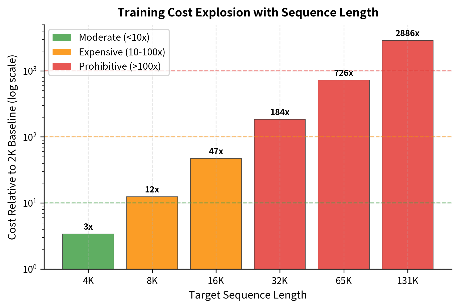
The numbers are stark. Training on 32K tokens costs roughly 180x more per sequence than training on 2K tokens. To maintain the same training throughput, you'd need 180x more compute budget. Alternatively, you accept 180x smaller effective batch sizes, which can destabilize training. Neither option is appealing.

The attention mechanism computes pairwise interactions between all tokens. For each layer and each attention head, we must store an $n \times n$ matrix of attention weights, where every entry $(i, j)$ represents how much token $i$ attends to token $j$. The total memory required to store these attention matrices is:

where:

• $M_{\text{attn}}$: total memory in bytes for all attention matrices
• $h$: number of attention heads (each head computes an independent attention pattern)
• $L$: number of transformer layers (each layer has its own set of attention matrices)
• $n$: sequence length in tokens
• $n^2$: the size of each attention matrix (one entry per query-key pair)
• $b$: bytes per element (2 for fp16/bf16, 4 for fp32)

The critical insight is that $n$ appears squared: doubling the sequence length quadruples the memory for attention matrices. This is the source of the quadratic memory scaling that limits context length.

But this formula only accounts for the attention weight matrices themselves. A complete picture of memory consumption includes:

• Key-value cache (for inference): $2 \times L \times n \times d$
• Activations (for training): Intermediate values needed for backpropagation
• Gradients: Same size as activations

For training, the numbers quickly become untenable. A 32K sequence requires over 500 GB for attention matrices alone, far exceeding any single GPU. Even with gradient checkpointing (recomputing activations during backprop instead of storing them), the attention matrices remain the bottleneck.

For inference, the KV cache dominates. At 128K tokens, storing keys and values for all layers consumes over 60 GB. This explains why long-context inference requires careful memory management and often multiple GPUs.

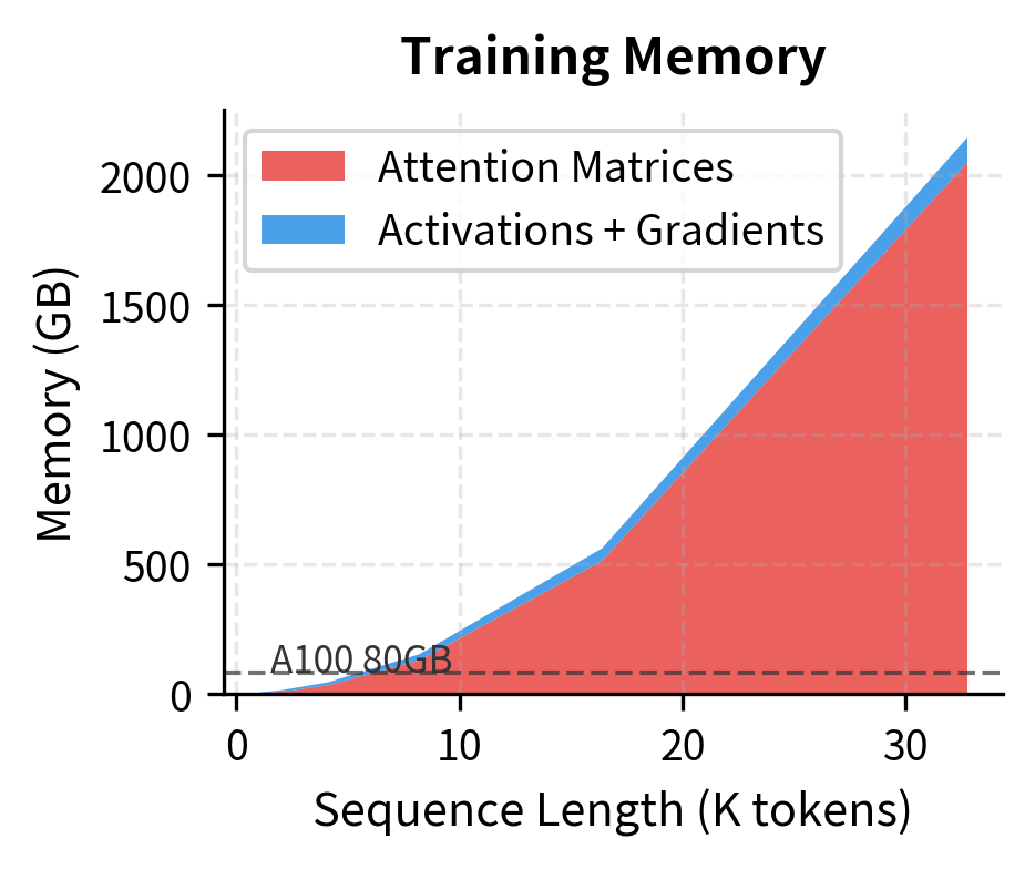
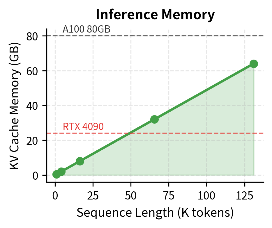
These visualizations reveal why long-context training and inference require fundamentally different approaches. Training hits the quadratic wall with attention matrices. Inference hits a linear wall with KV cache storage. Solutions like FlashAttention address the first problem by never materializing the full attention matrix. Solutions like KV cache compression and sliding window attention address the second.

Position encodings tell the model where each token sits in the sequence. Without them, attention treats "The cat sat on the mat" and "mat the on sat cat The" identically. The challenge: most position encoding schemes fail catastrophically when asked to encode positions beyond their training range.

The original transformer used learned absolute position embeddings: a lookup table mapping each position index to a learned vector. If you train with positions 0 through 511, the embedding table has 512 entries. What happens at position 512? The model has never seen it.

Absolute embeddings have zero ability to extrapolate. The model either crashes or produces garbage for unseen positions. This hard limit explains why early BERT applications required truncating documents to 512 tokens.

The original "Attention Is All You Need" paper proposed sinusoidal encodings that compute position vectors using trigonometric functions rather than learning them from data. The key idea is to create position-dependent patterns at multiple frequencies, allowing the model to detect both local and distant positional relationships.

For a position $pos$ in the sequence and dimension index $i$ in the encoding vector:

where:

• $PE_{(pos, 2i)}$: the encoding value at position $pos$ for even dimension $2i$
• $PE_{(pos, 2i+1)}$: the encoding value at position $pos$ for odd dimension $2i+1$
• $pos$: the absolute position in the sequence (0, 1, 2, ...)
• $i$: the dimension index within the encoding (ranges from 0 to $d/2 - 1$)
• $d$: the total dimensionality of the position encoding (typically matches the model's hidden dimension)
• $10000$: a base constant that determines the range of wavelengths

The division by $10000^{2i/d}$ creates different frequencies across dimensions. Low-indexed dimensions (small $i$) oscillate rapidly with position, while high-indexed dimensions oscillate slowly. This multi-scale representation allows the model to capture both fine-grained local position (from high-frequency components) and coarse global position (from low-frequency components).

Since these are deterministic mathematical functions rather than learned embeddings, they can generate vectors for any position, including positions never seen during training. But can the model actually use them beyond its training range?

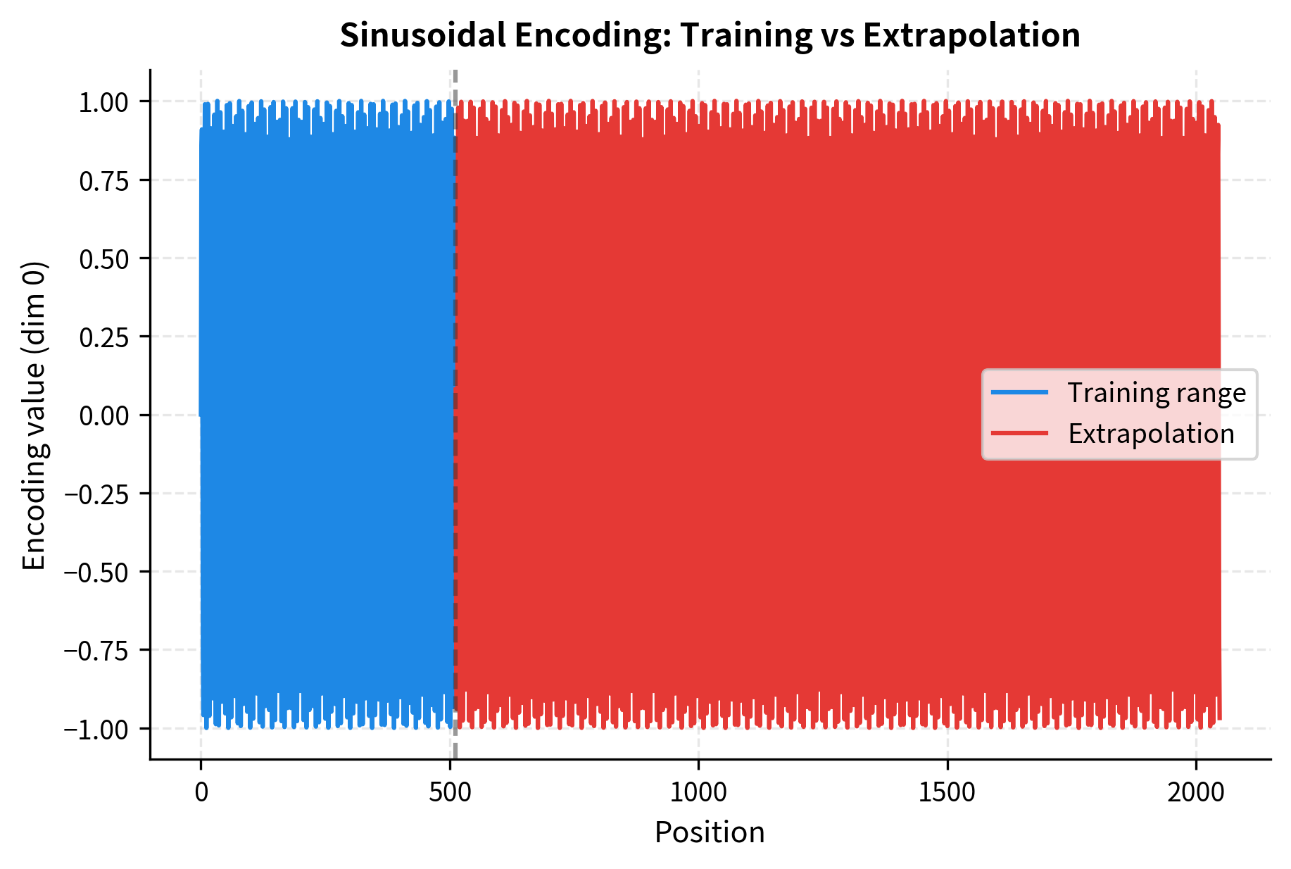
Sinusoidal encodings produce mathematically valid vectors at any position. The issue is semantic: the model learned to interpret positions 0-511 during training. Position 1024 might have a perfectly valid encoding, but the model hasn't learned what attention patterns make sense when tokens are that far apart.

Rotary Position Embeddings (RoPE), used in LLaMA and many modern models, encode relative positions through rotation in embedding space. They offer better extrapolation than absolute embeddings but still degrade beyond training length.

At position 4096 (2x training length), high-frequency components have rotated 163 times. At position 16384 (8x training length), they've rotated 653 times. The model has never seen these rotation patterns. The mismatch manifests as degraded attention: tokens that should attend to each other might not, and irrelevant tokens might receive spurious attention.

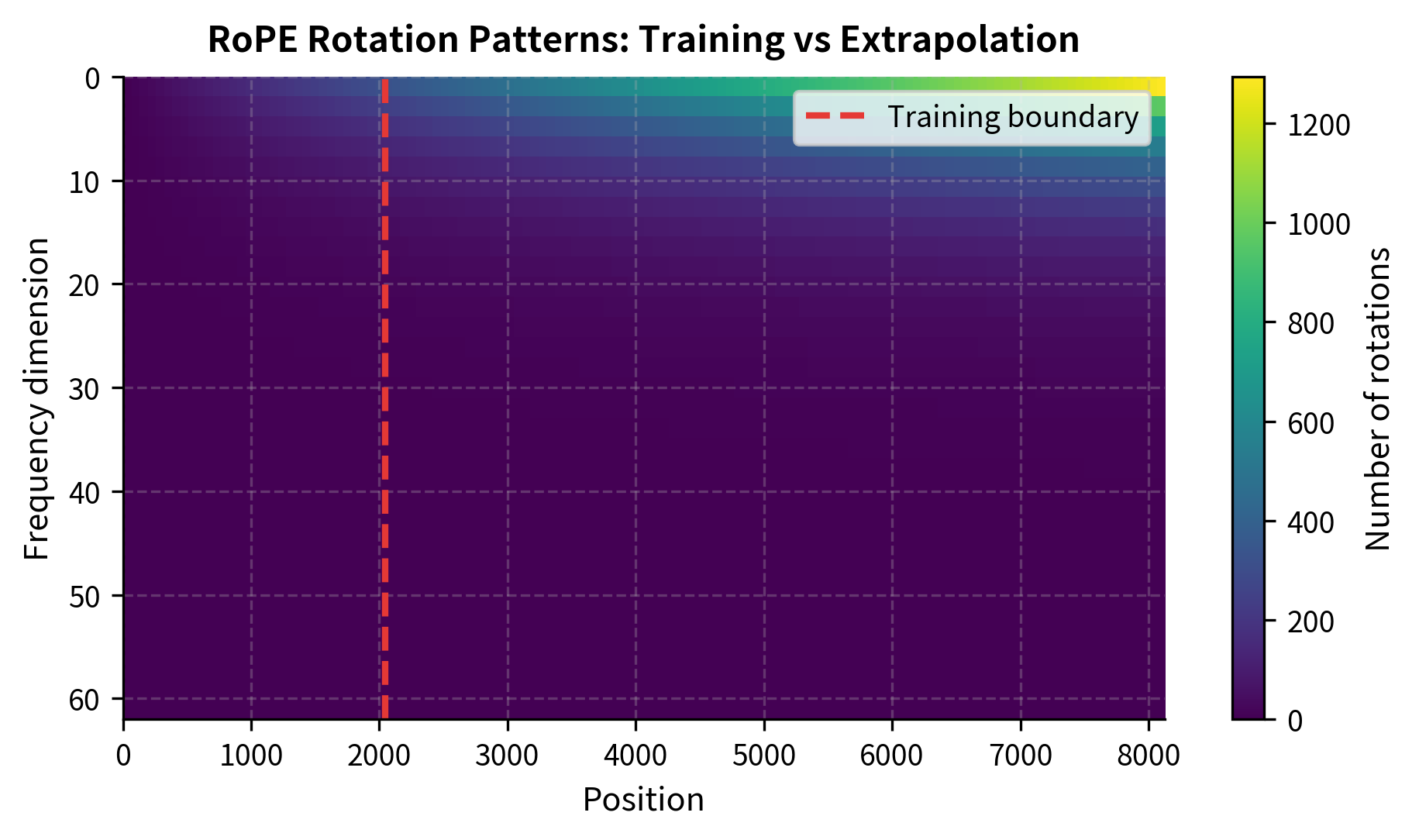
The visualization shows why position interpolation (covered in the next chapter) works: instead of asking the model to interpret new rotation regimes, we rescale positions to stay within the familiar training range. Position 4096 becomes position 2048, which the model understands.

Even if we solve the memory and position encoding problems, there's a more fundamental challenge: can models actually learn to use information from thousands of tokens ago?

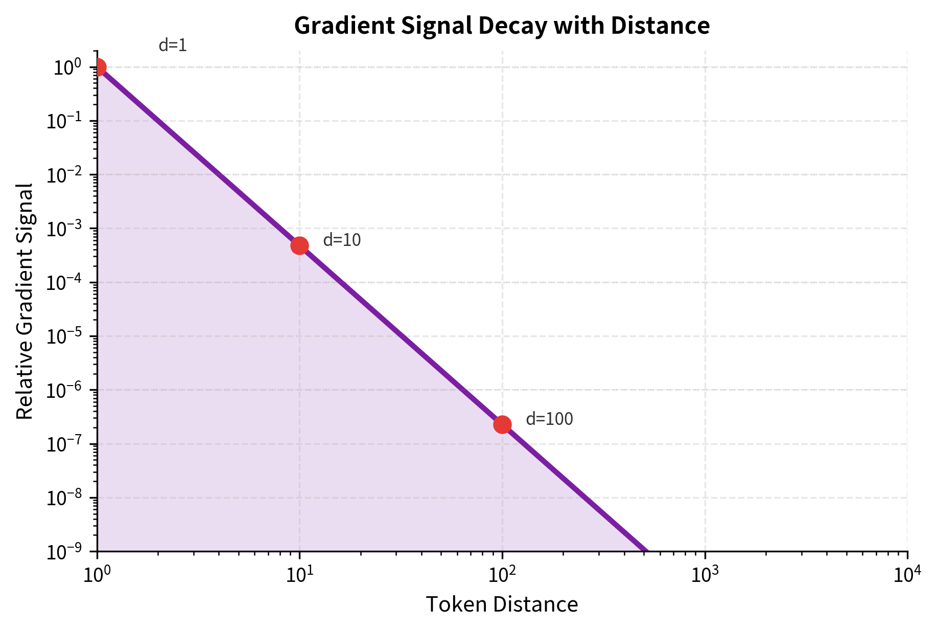
During training, the model must learn connections between distant tokens through backpropagation. For a dependency spanning 1000 tokens, gradients must flow through 1000 attention steps. Even with attention's direct connections, this creates challenges.

Consider a simple task: matching an opening bracket to its closing bracket. If they're 10 tokens apart, the model easily learns the pattern. If they're 1000 tokens apart, the signal becomes diluted.

The gradient signal drops by orders of magnitude as distance increases. At 1000 tokens, the signal is roughly 10 million times weaker than at distance 1. This doesn't mean learning is impossible, but it requires many more training examples to establish long-range patterns.

Attention weights must sum to 1 across all positions (due to softmax normalization). With uniform attention distributed equally over $n$ tokens, each token receives exactly $1/n$ of the total attention mass. As sequence length grows, this fraction shrinks proportionally: at $n = 100$ tokens, each token receives 1% of attention; at $n = 10{,}000$ tokens, each receives only 0.01%.

For long sequences, this means any single token contributes a tiny fraction to the output.

With uniform attention over 128K tokens, the 10 relevant tokens receive only 0.008% of attention mass combined. The signal is buried in noise. This is why models must learn to concentrate attention on relevant tokens. But learning that concentration itself requires seeing many examples where those long-range connections matter.

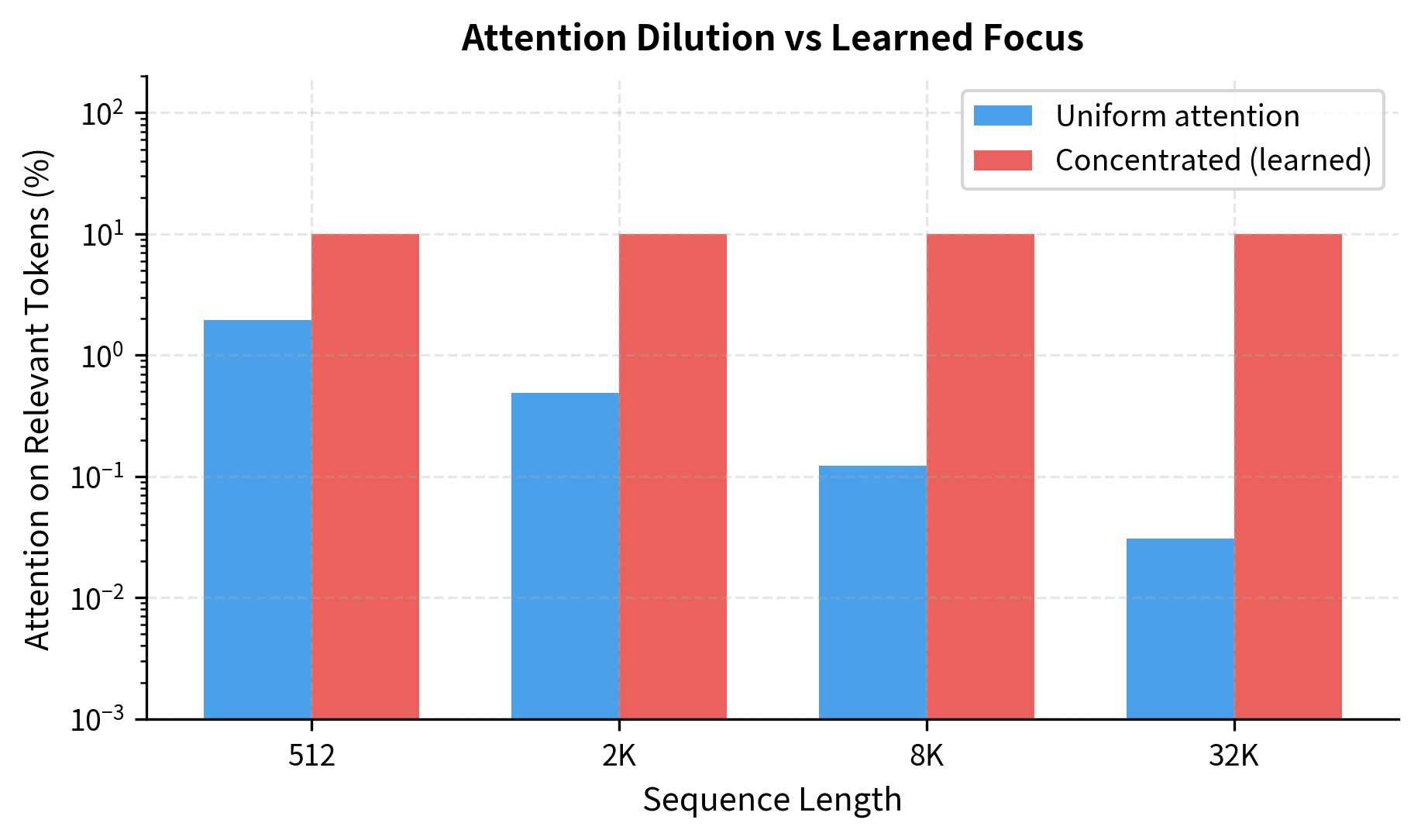
The visualization shows that learned concentration can maintain signal even at very long sequence lengths. But achieving this concentration requires training data where long-range dependencies matter and gradients that can reinforce the correct attention patterns.

How do we know if a model actually uses long context? Perplexity on long documents tells us the model predicts well overall, but not whether it's using information from 10K tokens ago. This evaluation gap has led to the development of specialized benchmarks.

The most intuitive test: hide a specific fact early in a long document, then ask about it at the end. If the model can retrieve the fact, it's using long context.

Real benchmarks like RULER and LongBench extend this idea with multiple needles, multi-hop reasoning, and varying distractor difficulty. Performance typically degrades as the needle moves earlier in the document, revealing the model's effective context utilization.

A harder test: require the model to combine information from multiple distant locations.

Multi-hop tests reveal whether models can maintain and combine information across distances. Many models that pass single-needle tests fail multi-hop tests, suggesting they struggle with genuine reasoning over long context rather than just retrieval.

A striking empirical finding: models often perform best when relevant information is at the beginning or end of the context, and worst when it's in the middle. This "lost in the middle" effect suggests attention doesn't uniformly cover the context.

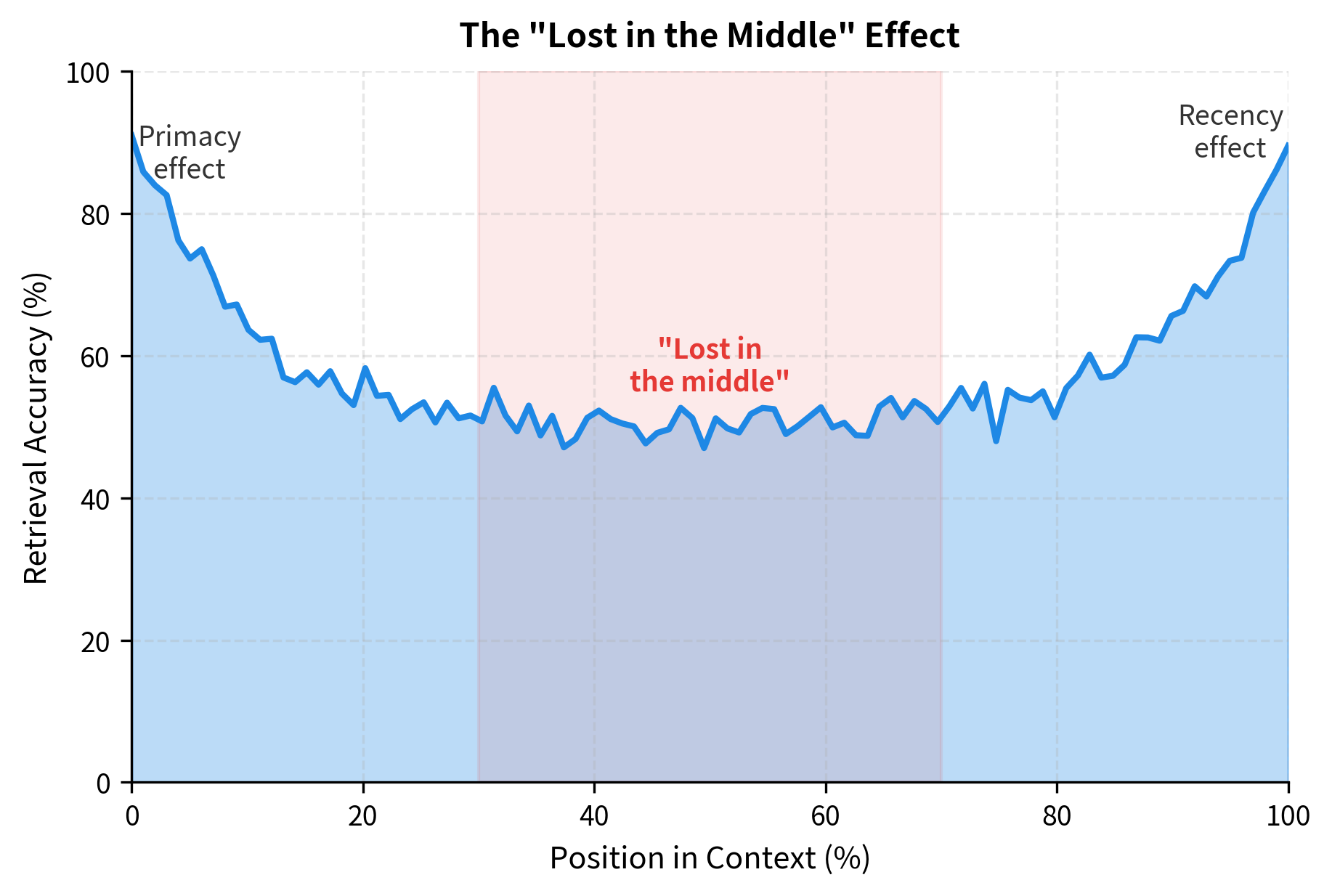
The "lost in the middle" effect has significant practical implications. When building RAG systems or structuring long prompts, placing critical information at the beginning or end improves retrieval. Understanding this phenomenon is essential for effective use of long-context models.

Let's bring together the challenges with a concrete example. We'll simulate how a model's performance degrades as we push beyond training context.

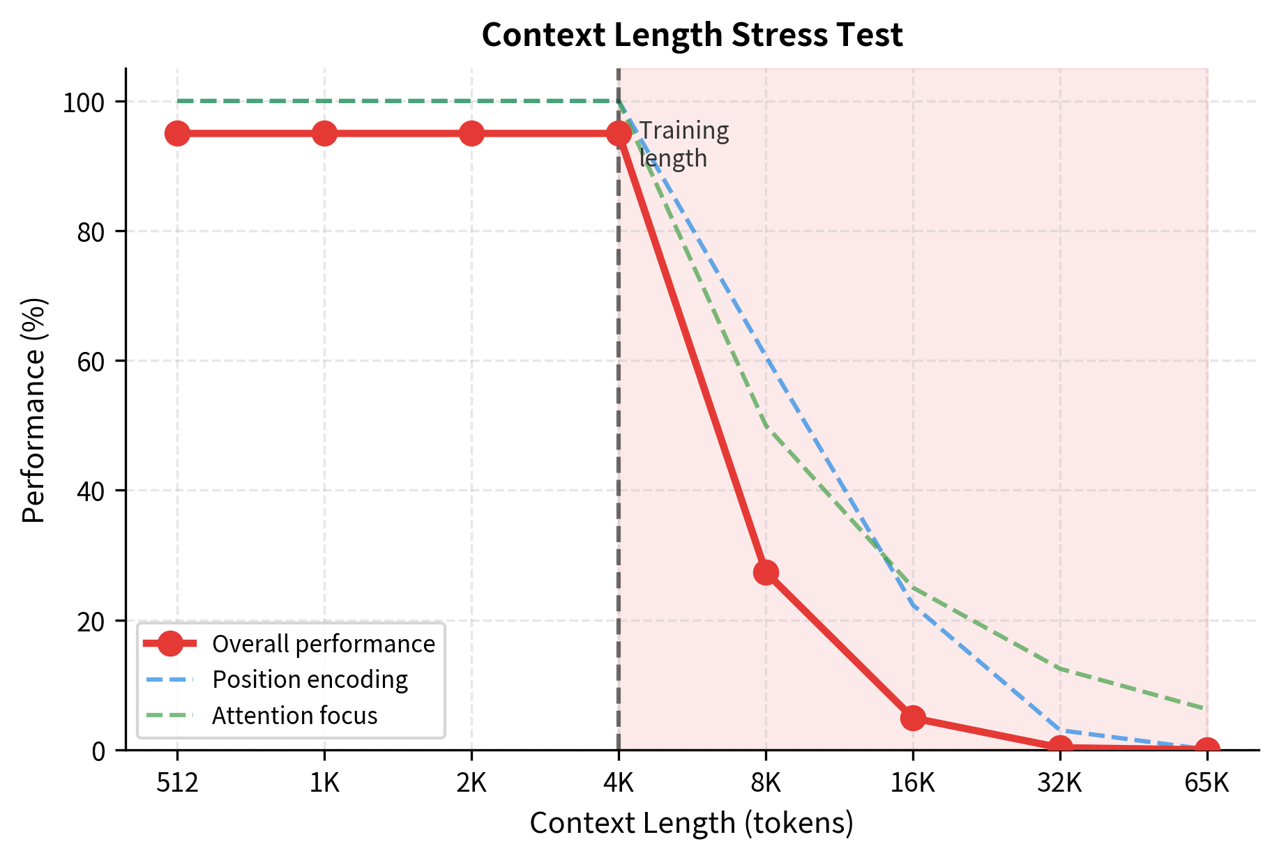
The stress test visualizes how multiple factors compound to degrade performance beyond training length. Position encoding breaks first and most severely. Attention dilution provides a gentler decay. Together, they explain why naive extrapolation fails and motivate the techniques covered in subsequent chapters.

The context length challenges we've examined create real limitations for language models in practice, but they've also driven innovation that has expanded what's possible.

Practical limitations remain significant. Even with 200K token context windows, models don't use all that context equally. The "lost in the middle" effect means critical information should be placed strategically. Multi-hop reasoning over very long distances remains unreliable. And the computational cost of long contexts limits their use in latency-sensitive applications.

Training costs scale prohibitively. Extending context length during training requires quadratically more compute for attention. Most long-context models are fine-tuned from shorter-context bases rather than trained from scratch, inheriting some limitations of the shorter training. True end-to-end training on 100K+ token sequences remains rare due to cost.

Evaluation doesn't capture everything. Needle-in-a-haystack tests measure retrieval but not reasoning. Models might locate information without understanding how to use it. Multi-hop benchmarks are better but still don't capture the full complexity of real-world long-document tasks like legal analysis or scientific synthesis.

Despite these challenges, the progress has been remarkable. In 2020, a 4K context window was generous. By 2024, 200K+ tokens became available. This expansion enables qualitatively new applications: analyzing entire codebases, processing full legal documents, and maintaining coherent multi-hour conversations. The techniques developed to overcome context length challenges, position interpolation, efficient attention, and memory augmentation, have become essential tools in the language modeling arsenal.

Understanding the fundamental challenges prepares us to appreciate the solutions. The next chapters explore position interpolation techniques that enable extrapolation, attention mechanisms that reduce the quadratic burden, and memory architectures that extend effective context beyond what fits in a single forward pass.

Context length limitations arise from multiple interacting factors, each creating its own barrier to long-document processing.

Training sequence limits are set by computational constraints. Both memory (quadratic in sequence length for attention matrices) and compute (also quadratic) restrict practical training lengths. Extending training length by 2x costs roughly 4x more resources.

Attention memory scaling follows $O(n^2)$ for attention matrices during training and $O(n)$ for KV cache during inference. A 32K sequence requires 256x more attention memory than a 1K sequence, quickly exceeding GPU limits.

Position encoding extrapolation fails for most schemes. Absolute embeddings cannot represent positions beyond training length. Sinusoidal and RoPE encodings can generate valid vectors but produce patterns the model hasn't learned to interpret. High-frequency components in RoPE rotate into unfamiliar regimes at long positions.

Long-range dependency learning struggles against gradient dilution and attention spread. Signals from distant tokens must compete against nearby context, and learning to focus on relevant distant tokens requires training examples where those dependencies matter.

Evaluation challenges make it hard to measure true context utilization. Simple perplexity hides whether models use distant context. Needle-in-a-haystack tests reveal retrieval ability but not reasoning. The "lost in the middle" effect shows that even large context windows don't guarantee uniform utilization.

These challenges are not insurmountable. Position interpolation, efficient attention, and memory augmentation, covered in the following chapters, each address specific aspects of the long-context problem. Understanding the challenges provides the foundation for appreciating the solutions.

When analyzing context length limitations or designing systems that work with long sequences, these parameters directly determine feasibility and performance:

• n (sequence length): The number of tokens in the input. This is the most critical parameter since both memory and compute scale with $n^2$ for attention. Typical values range from 512 (early BERT) to 1M+ (modern long-context models).

• h (number of attention heads): Each head stores an independent $n \times n$ attention matrix. Memory scales linearly with head count. Common values: 12 (GPT-2 Small) to 128 (large models).

• L (number of layers): Transformer depth. Both attention memory and KV cache scale linearly with layer count. Typical range: 12-96 layers.

• d (model dimension): The embedding size. KV cache scales as $O(L \times n \times d)$. Common values: 768 (BERT-base) to 8192 (large LLMs).

• dtype_bytes: Precision of stored values. Using fp16/bf16 (2 bytes) instead of fp32 (4 bytes) halves memory requirements. Most modern training uses bf16.

• training_length: The maximum sequence length seen during training. Determines the "safe" operating range for position encodings. Extrapolation beyond this length causes degradation unless mitigation techniques are applied.

• base (RoPE): The base constant in rotary position embeddings (default 10000). Affects the frequency spectrum of position encoding. Modifying this is one approach to extending context (NTK-aware scaling).

• window_size (sliding window attention): For models using local attention, this determines how many tokens each position can attend to. Larger windows capture more context but use more memory. Common values: 256-4096 tokens.

Ready to test your understanding? Take this quick quiz to reinforce what you've learned about the fundamental challenges limiting transformer context lengths.