Prefix Language Modeling: Combining Bidirectional Context with Causal Generation

Michael Brenndoerfer

Data, Analytics & AI Machine Learning Language AI Handbook

Master prefix LM, the hybrid pretraining objective that enables bidirectional prefix understanding with autoregressive generation. Covers T5, UniLM, and implementation.

Track your reading progress

Sign in to mark chapters as read and track your learning journey

Sign in →

Reading Level

Choose your expertise level to adjust how many terms are explained. Beginners see more tooltips, experts see fewer to maintain reading flow. Hover over underlined terms for instant definitions.

Prefix Language ModelingLink Copied

What if you could have the best of both worlds? Causal language modeling excels at generation but sees only left context. Masked language modeling captures bidirectional context but cannot generate text autoregressively. Prefix Language Modeling (Prefix LM) bridges this gap by treating part of the input bidirectionally and the rest causally, enabling models that both understand context deeply and generate fluently.

The key insight is simple: when generating a continuation of a prompt, the prompt itself is fully known. There's no reason to hide later prompt tokens from earlier ones. Only the generation, which unfolds token by token, requires causal masking. Prefix LM formalizes this intuition into a training objective that powers models like T5, UniLM, and UL2.

In this chapter, we'll explore the prefix LM formulation, understand its distinctive attention pattern, implement the objective from scratch, and examine how it enables unified models for both understanding and generation.

The Prefix LM IntuitionLink Copied

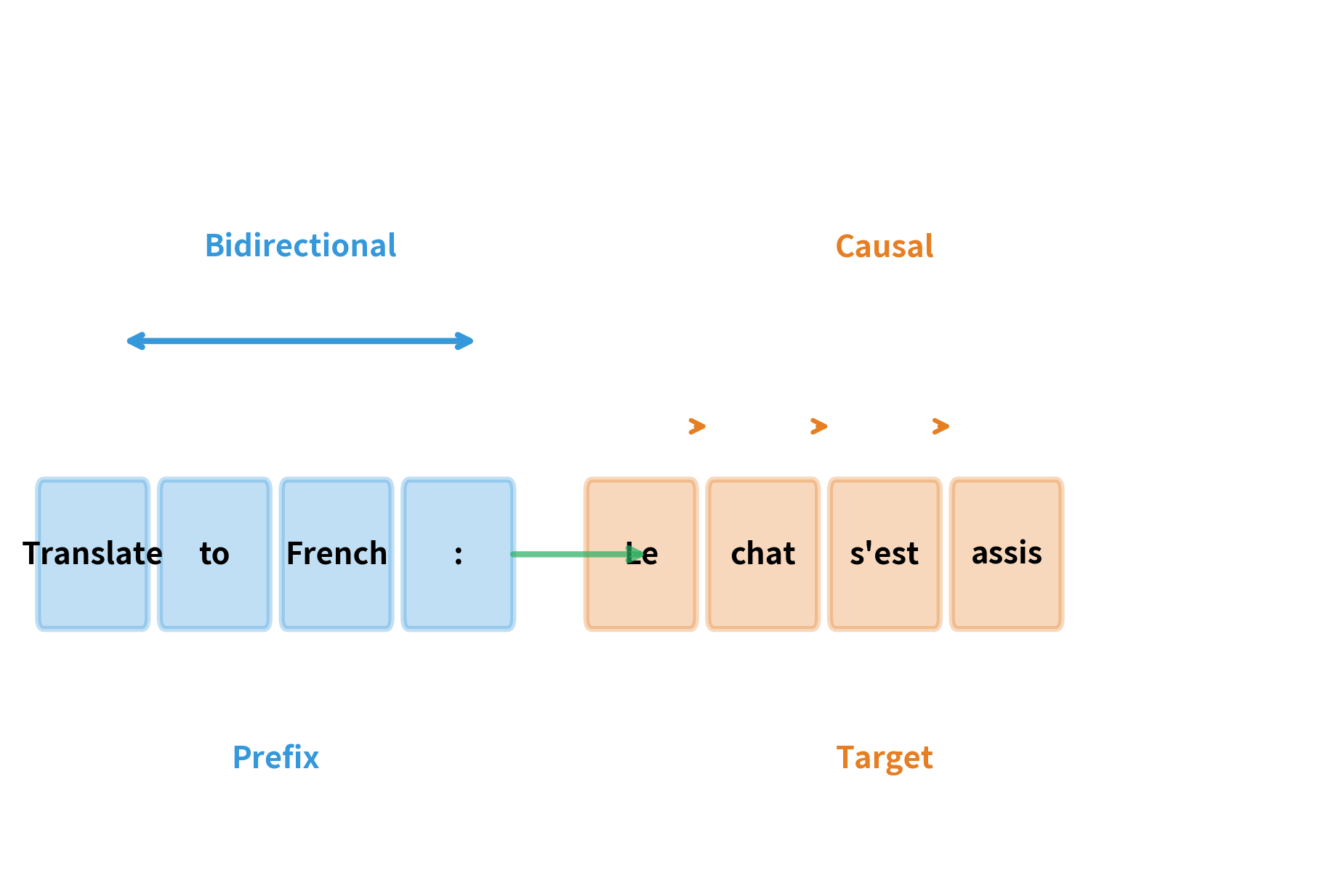
Consider a translation task: "Translate to French: The cat sat on the mat." The input prompt is complete and known. When generating "Le chat s'est assis sur le tapis," each French word depends on the entire English prompt plus previously generated French words. There's no benefit to hiding "mat" from "cat" in the English prompt.

Prefix LM captures this asymmetry. The sequence is split into two parts:

Prefix: The conditioning context (prompt, input, instruction). Tokens here can attend to each other bidirectionally.
Target: The continuation to be generated. Tokens here can attend to the full prefix plus their own left context, following causal constraints.

This hybrid attention pattern preserves the generation capability of causal LM while allowing richer representation of the prefix through bidirectional attention.

Out[3]:

Visualization

Diagram showing a sequence split into prefix and target regions with different attention patterns indicated by arrows. — Prefix language modeling splits the sequence into two regions. The prefix (blue) uses bidirectional attention where all tokens can see each other. The target (orange) uses causal attention, seeing the full prefix plus left context only. This hybrid approach combines the representational power of bidirectional models with the generation capability of autoregressive models.

This structure matches many real-world scenarios. In question answering, the question is the prefix and the answer is the target. In summarization, the document is the prefix and the summary is the target. In dialogue, the conversation history is the prefix and the next response is the target. The bidirectional prefix captures the full context, while the causal target enables coherent generation.

The Prefix LM ObjectiveLink Copied

Now that we understand the intuition behind splitting sequences into prefix and target regions, we need a formal training objective. The key question is: how do we mathematically express what we want the model to learn?

From Intuition to FormalizationLink Copied

Think about what happens when you complete someone's sentence. You don't just hear the first word and guess; you take in the entire context they've provided, then generate a continuation that fits seamlessly. Prefix LM captures exactly this: the model should fully understand the prefix before generating the target.

This leads to two requirements that our objective must encode:

Full prefix visibility: When predicting any target token, the model should have access to the complete prefix, not just the tokens that came before.
Causal target generation: Target tokens should be generated left-to-right, each depending on previous target tokens but not future ones.

The Mathematical FormulationLink Copied

Consider a sequence $x = (x_1, \ldots, x_n)$ divided at position $k$ into two parts: the prefix $x_{1:k} = (x_1, \ldots, x_k)$ and the target $x_{k+1:n} = (x_{k+1}, \ldots, x_n)$ . The training objective minimizes the negative log-likelihood of predicting target tokens:

\mathcal{L}_{\text{Prefix-LM}} = -\sum_{t=k+1}^{n} \log P_\theta(x_t | x_{1:k}, x_{k+1:t-1})

where:

$\mathcal{L}_{\text{Prefix-LM}}$ : the prefix language modeling loss to minimize
$n$ : the total sequence length
$k$ : the position where the prefix ends and the target begins (the split point)
$x_{1:k}$ : the prefix tokens $(x_1, \ldots, x_k)$ , which are fully visible bidirectionally
$x_{k+1:t-1}$ : the target tokens generated before position $t$ , specifically $(x_{k+1}, \ldots, x_{t-1})$
$P_\theta(x_t | x_{1:k}, x_{k+1:t-1})$ : the probability the model with parameters $\theta$ assigns to token $x_t$ , conditioned on the full prefix and all preceding target tokens
The summation $\sum_{t=k+1}^{n}$ iterates only over target positions, from $k+1$ to $n$

Understanding the ConditioningLink Copied

The heart of this formula lies in the conditioning term $x_{1:k}, x_{k+1:t-1}$ . Let's unpack what this means for a concrete example.

Suppose we have the sequence "The cat sat on the mat" with $k=3$ (prefix is "The cat sat"). When predicting the fourth word "on":

The model sees: all of "The cat sat" (bidirectionally) + nothing yet from the target
When predicting "the": sees "The cat sat" + "on"
When predicting "mat": sees "The cat sat" + "on the"

Notice the asymmetry: prefix tokens are always fully visible, while target tokens accumulate causally. This is the mathematical expression of the L-shaped attention mask we'll implement shortly.

Why Loss on Target Only?Link Copied

The loss summation starts at $k+1$ , not at 1. This means we compute loss only on target tokens, ignoring prefix tokens entirely. Why?

The prefix is given as input at inference time. Asking the model to predict prefix tokens would be like testing whether someone can recite back what you just told them. That's not the skill we want to develop. Instead, we focus all learning signal on the generation task: given this context, what comes next?

This differs from causal LM, where every position contributes to the loss. In prefix LM, the prefix serves purely as conditioning context, its representation is refined through gradient flow, but no direct prediction loss applies to it.

Prefix Language Modeling

A pretraining objective that splits sequences into a prefix with bidirectional attention and a target with causal attention. The model learns to generate the target conditioned on the full bidirectional context of the prefix, combining the representational power of encoder-style models with the generation capability of decoder-style models.

The Prefix LM Attention PatternLink Copied

The mathematical objective we just defined has a direct physical manifestation: the attention mask. This mask controls which tokens can "see" which other tokens during the forward pass, and it must encode our two key requirements: bidirectional prefix and causal target.

Unlike the uniform lower-triangular mask of causal LM or the full-attention mask of masked LM, prefix LM uses a hybrid pattern that changes behavior partway through the sequence.

Out[4]:

Visualization

Heatmap showing attention mask with full attention in upper-left prefix region and causal triangular pattern in lower-right target region. — The prefix LM attention mask combines bidirectional and causal patterns. The prefix region (positions 0-3) has full attention where all tokens attend to each other. The target region (positions 4-7) uses causal attention, attending to the full prefix plus left context only. This creates the characteristic L-shaped pattern.

Anatomy of the Attention MaskLink Copied

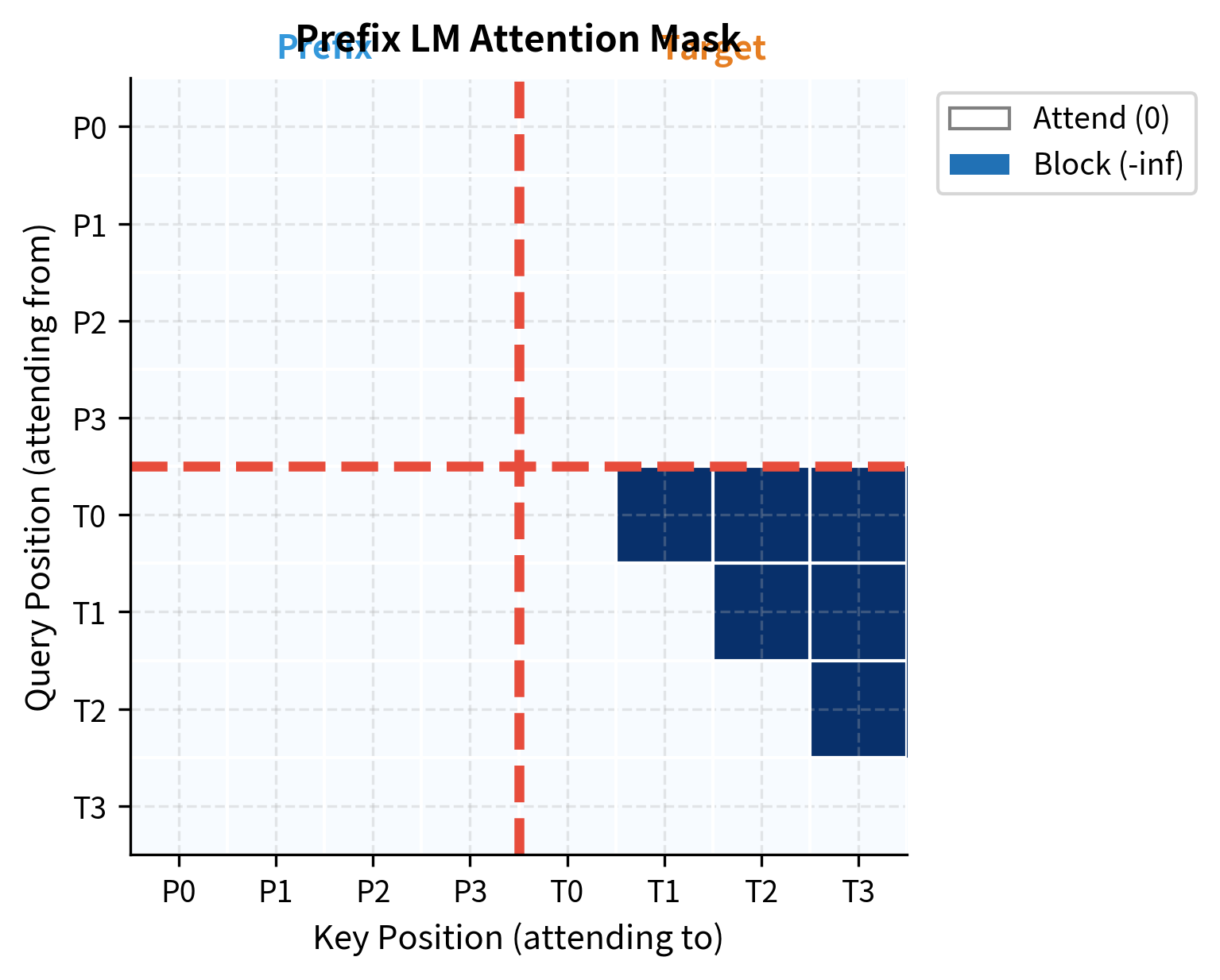
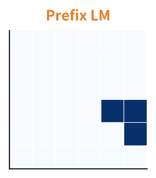
The mask divides naturally into three regions, each serving a distinct purpose:

Prefix-to-prefix (upper-left quadrant): Full bidirectional attention. Every prefix token attends to every other prefix token, and can also attend to all target positions. This is what gives the prefix its representational richness, as each word can incorporate context from the entire sequence.
Target-to-prefix (lower-left rectangle): Full attention. Every target token attends to all prefix tokens. This is how the conditioning flows, when generating "Le" in our translation example, the model can look back at any part of "Translate to French: The cat sat on the mat."
Target-to-target (lower-right quadrant): Causal attention. Each target token attends only to itself and preceding target tokens. This preserves the autoregressive property needed for generation, you can't peek at future words you haven't generated yet.

Together, these regions create the characteristic L-shaped pattern visible in the mask visualization. The prefix forms a fully connected subgraph where information flows freely in all directions, while the target maintains causal structure that enables token-by-token generation.

Implementing the MaskLink Copied

Translating this pattern into code requires building a matrix where each entry indicates whether position $i$ can attend to position $j$ :

In[5]:

Code

def create_prefix_lm_mask(seq_len, prefix_len):
    """
    Create attention mask for prefix language modeling.

    Args:
        seq_len: Total sequence length
        prefix_len: Length of the prefix (bidirectional) region

    Returns:
        Mask where 0 indicates attend, -inf indicates block
    """
    # Start with zeros (all attend)
    mask = torch.zeros(seq_len, seq_len)

    # For target positions (after prefix), apply causal masking
    for i in range(prefix_len, seq_len):
        for j in range(i + 1, seq_len):
            mask[i, j] = float("-inf")

    return mask

def create_prefix_lm_mask(seq_len, prefix_len):
    """
    Create attention mask for prefix language modeling.

    Args:
        seq_len: Total sequence length
        prefix_len: Length of the prefix (bidirectional) region

    Returns:
        Mask where 0 indicates attend, -inf indicates block
    """
    # Start with zeros (all attend)
    mask = torch.zeros(seq_len, seq_len)

    # For target positions (after prefix), apply causal masking
    for i in range(prefix_len, seq_len):
        for j in range(i + 1, seq_len):
            mask[i, j] = float("-inf")

    return mask

Out[6]:

Console

Prefix LM mask (8 positions, prefix_len=4):
(0 = attend, -inf = block)

Pos 0: [  0 ,   0 ,   0 ,   0 ,   0 ,   0 ,   0 ,   0 ]
Pos 1: [  0 ,   0 ,   0 ,   0 ,   0 ,   0 ,   0 ,   0 ]
Pos 2: [  0 ,   0 ,   0 ,   0 ,   0 ,   0 ,   0 ,   0 ]
Pos 3: [  0 ,   0 ,   0 ,   0 ,   0 ,   0 ,   0 ,   0 ]
Pos 4: [  0 ,   0 ,   0 ,   0 ,   0 , -inf, -inf, -inf]
Pos 5: [  0 ,   0 ,   0 ,   0 ,   0 ,   0 , -inf, -inf]
Pos 6: [  0 ,   0 ,   0 ,   0 ,   0 ,   0 ,   0 , -inf]
Pos 7: [  0 ,   0 ,   0 ,   0 ,   0 ,   0 ,   0 ,   0 ]

The first four positions (prefix) have all zeros, meaning they attend to everything. Positions 4-7 (target) have zeros up to and including their own position, then negative infinity to block future tokens.

Comparing Attention PatternsLink Copied

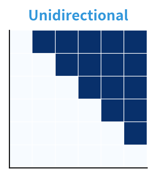
To understand prefix LM's unique position, let's compare it with causal and masked LM attention patterns:

Out[7]:

Visualization

Lower triangular attention matrix for causal LM. — Causal LM: Each position attends only to itself and earlier positions, enforcing strict left-to-right information flow.

Full attention matrix for masked LM. — Masked LM: Full bidirectional attention where every position attends to every other position.

L-shaped attention matrix for prefix LM with bidirectional prefix and causal target. — Prefix LM: Hybrid pattern with bidirectional prefix and causal target, capturing context richly while enabling generation.

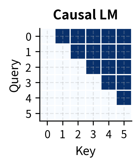
The visual comparison reveals the key differences:

Comparison of attention patterns across language modeling objectives.

Aspect	Causal LM	Masked LM	Prefix LM
Prefix attention	Causal	Bidirectional	Bidirectional
Target attention	Causal	Bidirectional	Causal
Generation	Yes	No	Yes
Context richness	Limited	Full	Hybrid
Use case	Pure generation	Understanding	Conditioned generation

Prefix LM occupies the middle ground. It enables generation like causal LM while providing richer prefix representations like masked LM.

Out[8]:

Visualization

Line plot comparing attention span across positions for causal LM, masked LM, and prefix LM, showing prefix LM's hybrid behavior. — Number of positions each token can attend to across different LM objectives. Causal LM (blue) shows linear growth from 1 to n. Masked LM (green) provides full access to all n positions. Prefix LM (orange) has full access for prefix positions, then follows the causal pattern for target positions. The shaded region highlights the advantage Prefix LM gains in the prefix region.

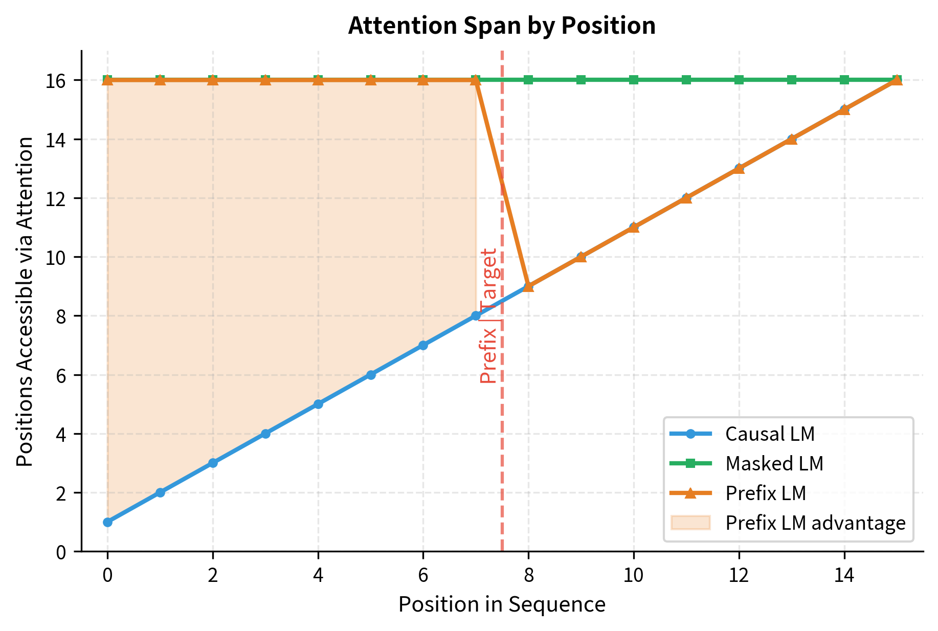
This plot quantifies the representational advantage of prefix LM. In the prefix region (positions 0-7), each token has full access to all 16 positions, just like masked LM. In the target region (positions 8-15), the attention span follows the causal pattern, growing linearly. The shaded area represents the additional context each prefix position gains compared to causal LM, which translates to richer representations that inform target generation.

Implementing Prefix LM TrainingLink Copied

With the mathematical foundation and attention pattern in place, we can now build a complete prefix LM from scratch. This implementation brings together everything we've discussed: the hybrid attention mask, the target-only loss computation, and the conditioning structure that makes prefix LM unique.

We'll construct the model in three stages: first the attention mechanism that applies our L-shaped mask, then the full transformer architecture, and finally the loss function that focuses learning on target positions.

The Attention MechanismLink Copied

The core innovation happens in the attention layer. We need to apply the prefix LM mask during the attention computation, ensuring that information flows according to our bidirectional-prefix, causal-target pattern:

In[9]:

Code

class PrefixLMAttention(nn.Module):
    """Multi-head attention with prefix LM masking."""

    def __init__(self, d_model, n_heads):
        super().__init__()
        self.d_model = d_model
        self.n_heads = n_heads
        self.head_dim = d_model // n_heads

        self.q_proj = nn.Linear(d_model, d_model)
        self.k_proj = nn.Linear(d_model, d_model)
        self.v_proj = nn.Linear(d_model, d_model)
        self.out_proj = nn.Linear(d_model, d_model)

    def forward(self, x, prefix_len):
        batch_size, seq_len, _ = x.shape

        # Project to Q, K, V
        q = self.q_proj(x).view(
            batch_size, seq_len, self.n_heads, self.head_dim
        )
        k = self.k_proj(x).view(
            batch_size, seq_len, self.n_heads, self.head_dim
        )
        v = self.v_proj(x).view(
            batch_size, seq_len, self.n_heads, self.head_dim
        )

        # Transpose for attention: (batch, heads, seq, head_dim)
        q = q.transpose(1, 2)
        k = k.transpose(1, 2)
        v = v.transpose(1, 2)

        # Compute attention scores
        scores = torch.matmul(q, k.transpose(-2, -1)) / (self.head_dim**0.5)

        # Apply prefix LM mask
        mask = create_prefix_lm_mask(seq_len, prefix_len).to(x.device)
        scores = scores + mask

        # Softmax and apply to values
        attn_weights = F.softmax(scores, dim=-1)
        output = torch.matmul(attn_weights, v)

        # Reshape and project
        output = (
            output.transpose(1, 2)
            .contiguous()
            .view(batch_size, seq_len, self.d_model)
        )
        return self.out_proj(output)

class PrefixLMAttention(nn.Module):
    """Multi-head attention with prefix LM masking."""

    def __init__(self, d_model, n_heads):
        super().__init__()
        self.d_model = d_model
        self.n_heads = n_heads
        self.head_dim = d_model // n_heads

        self.q_proj = nn.Linear(d_model, d_model)
        self.k_proj = nn.Linear(d_model, d_model)
        self.v_proj = nn.Linear(d_model, d_model)
        self.out_proj = nn.Linear(d_model, d_model)

    def forward(self, x, prefix_len):
        batch_size, seq_len, _ = x.shape

        # Project to Q, K, V
        q = self.q_proj(x).view(
            batch_size, seq_len, self.n_heads, self.head_dim
        )
        k = self.k_proj(x).view(
            batch_size, seq_len, self.n_heads, self.head_dim
        )
        v = self.v_proj(x).view(
            batch_size, seq_len, self.n_heads, self.head_dim
        )

        # Transpose for attention: (batch, heads, seq, head_dim)
        q = q.transpose(1, 2)
        k = k.transpose(1, 2)
        v = v.transpose(1, 2)

        # Compute attention scores
        scores = torch.matmul(q, k.transpose(-2, -1)) / (self.head_dim**0.5)

        # Apply prefix LM mask
        mask = create_prefix_lm_mask(seq_len, prefix_len).to(x.device)
        scores = scores + mask

        # Softmax and apply to values
        attn_weights = F.softmax(scores, dim=-1)
        output = torch.matmul(attn_weights, v)

        # Reshape and project
        output = (
            output.transpose(1, 2)
            .contiguous()
            .view(batch_size, seq_len, self.d_model)
        )
        return self.out_proj(output)

The key line is scores = scores + mask. By adding negative infinity to positions we want to block, the subsequent softmax converts those positions to zero probability. The mask is created dynamically based on prefix_len, allowing different sequences in a batch to have different split points.

The Complete ModelLink Copied

Now we wrap this attention mechanism in a full transformer architecture. The model includes embeddings, multiple transformer layers with our prefix LM attention, and an output projection to vocabulary logits:

In[10]:

Code

class TinyPrefixLM(nn.Module):
    """Minimal prefix language model for demonstration."""

    def __init__(
        self, vocab_size, d_model=128, n_heads=4, n_layers=2, max_len=128
    ):
        super().__init__()

        # Embeddings
        self.token_emb = nn.Embedding(vocab_size, d_model)
        self.pos_emb = nn.Embedding(max_len, d_model)
        self.layer_norm = nn.LayerNorm(d_model)
        self.dropout = nn.Dropout(0.1)

        # Attention layers
        self.attention_layers = nn.ModuleList(
            [PrefixLMAttention(d_model, n_heads) for _ in range(n_layers)]
        )

        # Feed-forward layers
        self.ff_layers = nn.ModuleList(
            [
                nn.Sequential(
                    nn.Linear(d_model, d_model * 4),
                    nn.GELU(),
                    nn.Linear(d_model * 4, d_model),
                    nn.Dropout(0.1),
                )
                for _ in range(n_layers)
            ]
        )

        # Layer norms
        self.attn_norms = nn.ModuleList(
            [nn.LayerNorm(d_model) for _ in range(n_layers)]
        )
        self.ff_norms = nn.ModuleList(
            [nn.LayerNorm(d_model) for _ in range(n_layers)]
        )

        # Output projection
        self.output = nn.Linear(d_model, vocab_size)

    def forward(self, x, prefix_len):
        batch_size, seq_len = x.shape

        # Embeddings
        positions = torch.arange(seq_len, device=x.device).unsqueeze(0)
        h = self.token_emb(x) + self.pos_emb(positions)
        h = self.layer_norm(h)
        h = self.dropout(h)

        # Transformer layers with prefix LM attention
        for attn, ff, attn_norm, ff_norm in zip(
            self.attention_layers,
            self.ff_layers,
            self.attn_norms,
            self.ff_norms,
        ):
            # Self-attention with residual
            h = h + attn(attn_norm(h), prefix_len)
            # Feed-forward with residual
            h = h + ff(ff_norm(h))

        # Project to vocabulary
        logits = self.output(h)
        return logits


def compute_prefix_lm_loss(logits, targets, prefix_len):
    """Compute loss only on target positions (after prefix)."""
    # Only compute loss on positions after the prefix
    target_logits = logits[:, prefix_len:, :]
    target_labels = targets[:, prefix_len:]

    # Flatten and compute cross-entropy
    vocab_size = logits.size(-1)
    loss = F.cross_entropy(
        target_logits.reshape(-1, vocab_size),
        target_labels.reshape(-1),
        ignore_index=-100,
    )
    return loss

class TinyPrefixLM(nn.Module):
    """Minimal prefix language model for demonstration."""

    def __init__(
        self, vocab_size, d_model=128, n_heads=4, n_layers=2, max_len=128
    ):
        super().__init__()

        # Embeddings
        self.token_emb = nn.Embedding(vocab_size, d_model)
        self.pos_emb = nn.Embedding(max_len, d_model)
        self.layer_norm = nn.LayerNorm(d_model)
        self.dropout = nn.Dropout(0.1)

        # Attention layers
        self.attention_layers = nn.ModuleList(
            [PrefixLMAttention(d_model, n_heads) for _ in range(n_layers)]
        )

        # Feed-forward layers
        self.ff_layers = nn.ModuleList(
            [
                nn.Sequential(
                    nn.Linear(d_model, d_model * 4),
                    nn.GELU(),
                    nn.Linear(d_model * 4, d_model),
                    nn.Dropout(0.1),
                )
                for _ in range(n_layers)
            ]
        )

        # Layer norms
        self.attn_norms = nn.ModuleList(
            [nn.LayerNorm(d_model) for _ in range(n_layers)]
        )
        self.ff_norms = nn.ModuleList(
            [nn.LayerNorm(d_model) for _ in range(n_layers)]
        )

        # Output projection
        self.output = nn.Linear(d_model, vocab_size)

    def forward(self, x, prefix_len):
        batch_size, seq_len = x.shape

        # Embeddings
        positions = torch.arange(seq_len, device=x.device).unsqueeze(0)
        h = self.token_emb(x) + self.pos_emb(positions)
        h = self.layer_norm(h)
        h = self.dropout(h)

        # Transformer layers with prefix LM attention
        for attn, ff, attn_norm, ff_norm in zip(
            self.attention_layers,
            self.ff_layers,
            self.attn_norms,
            self.ff_norms,
        ):
            # Self-attention with residual
            h = h + attn(attn_norm(h), prefix_len)
            # Feed-forward with residual
            h = h + ff(ff_norm(h))

        # Project to vocabulary
        logits = self.output(h)
        return logits


def compute_prefix_lm_loss(logits, targets, prefix_len):
    """Compute loss only on target positions (after prefix)."""
    # Only compute loss on positions after the prefix
    target_logits = logits[:, prefix_len:, :]
    target_labels = targets[:, prefix_len:]

    # Flatten and compute cross-entropy
    vocab_size = logits.size(-1)
    loss = F.cross_entropy(
        target_logits.reshape(-1, vocab_size),
        target_labels.reshape(-1),
        ignore_index=-100,
    )
    return loss

Notice how compute_prefix_lm_loss implements the target-only loss from our mathematical formulation. By slicing logits[:, prefix_len:, :], we extract only the predictions for target positions. The model produces logits for all positions (including the prefix), but we discard the prefix predictions when computing the loss, focusing the learning signal entirely on the generation task.

Out[11]:

Console

Model parameters: 670,184

Architecture:
  - Embedding dim: 128
  - Attention heads: 4
  - Layers: 2
  - Vocabulary: 1000

The model applies prefix LM attention in each layer, passing the prefix length to determine where the bidirectional/causal boundary lies. This is more flexible than hardcoding the mask, as different examples in a batch could have different prefix lengths.

Training on Prefix-Target PairsLink Copied

With our model architecture complete, we can now see prefix LM in action. We'll train on a simple task: given the first part of a sentence (the prefix), generate a plausible continuation (the target). Character-level tokenization keeps things interpretable, letting us watch the model learn character-by-character patterns.

Preparing the DataLink Copied

First, we create a small corpus and tokenize it at the character level:

In[12]:

Code

# Training corpus
text = """The quick brown fox jumps over the lazy dog.
A journey of a thousand miles begins with a single step.
To be or not to be that is the question.
All that glitters is not gold.
Knowledge is power and power is knowledge."""

# Character-level tokenization
chars = sorted(set(text))
char_to_idx = {c: i for i, c in enumerate(chars)}
idx_to_char = {i: c for c, i in char_to_idx.items()}
vocab_size = len(chars)

# Encode text
encoded = torch.tensor([char_to_idx[c] for c in text])

# Training corpus
text = """The quick brown fox jumps over the lazy dog.
A journey of a thousand miles begins with a single step.
To be or not to be that is the question.
All that glitters is not gold.
Knowledge is power and power is knowledge."""

# Character-level tokenization
chars = sorted(set(text))
char_to_idx = {c: i for i, c in enumerate(chars)}
idx_to_char = {i: c for c, i in char_to_idx.items()}
vocab_size = len(chars)

# Encode text
encoded = torch.tensor([char_to_idx[c] for c in text])

Out[13]:

Console

Vocabulary size: 32 characters
Text length: 216 characters
Sample: 'The quick brown fox jumps over the lazy dog.
A jou...'

This tiny corpus is far smaller than what you'd use for real pretraining, but it's enough to demonstrate the mechanics. The vocabulary of unique characters becomes our token space.

The Training Loop with Random SplitsLink Copied

A key design choice in prefix LM training is how to select the split point. We could fix it (always split at position 10), but that would limit generalization. Instead, we randomize the prefix length within a reasonable range. This teaches the model to handle varying amounts of context:

In[14]:

Code

def get_prefix_lm_batch(
    data, batch_size=16, seq_len=48, min_prefix_frac=0.3, max_prefix_frac=0.7
):
    """
    Create a batch for prefix LM training.

    Each sequence is split at a random point into prefix and target.
    The prefix fraction is randomly sampled between min and max.
    """
    # Sample random starting positions
    starts = torch.randint(0, len(data) - seq_len, (batch_size,))
    sequences = torch.stack([data[s : s + seq_len] for s in starts])

    # Random prefix length for this batch (same for all sequences in batch)
    prefix_frac = (
        torch.rand(1).item() * (max_prefix_frac - min_prefix_frac)
        + min_prefix_frac
    )
    prefix_len = int(seq_len * prefix_frac)

    # Input is the full sequence, target is shifted by 1
    input_ids = sequences[:, :-1]
    labels = sequences[:, 1:]

    # Adjust prefix_len for the shifted sequences
    prefix_len = max(1, prefix_len - 1)

    return input_ids, labels, prefix_len


# Training loop
model = TinyPrefixLM(vocab_size, d_model=64, n_heads=4, n_layers=2)
optimizer = torch.optim.AdamW(model.parameters(), lr=1e-3)

losses = []
for step in range(500):
    input_ids, labels, prefix_len = get_prefix_lm_batch(
        encoded, batch_size=8, seq_len=48
    )

    # Forward pass
    logits = model(input_ids, prefix_len)

    # Compute loss only on target (non-prefix) positions
    loss = compute_prefix_lm_loss(logits, labels, prefix_len)

    # Backward pass
    optimizer.zero_grad()
    loss.backward()
    optimizer.step()

    losses.append(loss.item())

def get_prefix_lm_batch(
    data, batch_size=16, seq_len=48, min_prefix_frac=0.3, max_prefix_frac=0.7
):
    """
    Create a batch for prefix LM training.

    Each sequence is split at a random point into prefix and target.
    The prefix fraction is randomly sampled between min and max.
    """
    # Sample random starting positions
    starts = torch.randint(0, len(data) - seq_len, (batch_size,))
    sequences = torch.stack([data[s : s + seq_len] for s in starts])

    # Random prefix length for this batch (same for all sequences in batch)
    prefix_frac = (
        torch.rand(1).item() * (max_prefix_frac - min_prefix_frac)
        + min_prefix_frac
    )
    prefix_len = int(seq_len * prefix_frac)

    # Input is the full sequence, target is shifted by 1
    input_ids = sequences[:, :-1]
    labels = sequences[:, 1:]

    # Adjust prefix_len for the shifted sequences
    prefix_len = max(1, prefix_len - 1)

    return input_ids, labels, prefix_len


# Training loop
model = TinyPrefixLM(vocab_size, d_model=64, n_heads=4, n_layers=2)
optimizer = torch.optim.AdamW(model.parameters(), lr=1e-3)

losses = []
for step in range(500):
    input_ids, labels, prefix_len = get_prefix_lm_batch(
        encoded, batch_size=8, seq_len=48
    )

    # Forward pass
    logits = model(input_ids, prefix_len)

    # Compute loss only on target (non-prefix) positions
    loss = compute_prefix_lm_loss(logits, labels, prefix_len)

    # Backward pass
    optimizer.zero_grad()
    loss.backward()
    optimizer.step()

    losses.append(loss.item())

Out[15]:

Console

Initial loss: 3.8094
Final loss: 0.4233
Random baseline: 3.4657
Loss reduction: 88.9%

The loss dropped substantially from the random baseline, indicating the model has learned meaningful patterns. A random model would assign equal probability to each token, yielding loss near the random baseline. The significant reduction shows the model is successfully using the bidirectional prefix context to improve target predictions.

Out[16]:

Visualization

Line plot showing prefix LM training loss decreasing from around 3.5 to 1.5 over 500 training steps. — Training loss for the prefix LM model. The loss is computed only on target positions (after the prefix), measuring how well the model generates continuations given the bidirectional prefix context. The rapid decrease indicates the model is learning to use the rich prefix representation for generation.

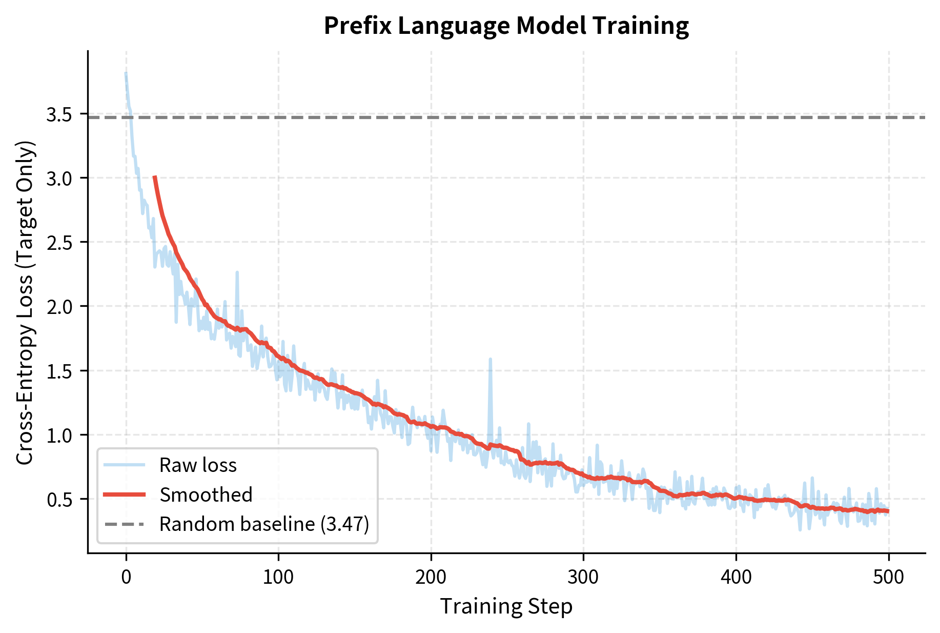
The model learns to generate continuations conditioned on the prefix. Unlike standard causal LM where loss is computed everywhere, prefix LM focuses the learning signal on the generation task. The prefix serves as rich context, processed bidirectionally, that informs the target generation.

Out[17]:

Visualization

Bar chart showing average loss increasing slightly for later target positions. — Average cross-entropy loss by target position (relative to prefix end). Position 0 is the first target token, immediately following the prefix. Earlier target positions typically have lower loss because they benefit most directly from the bidirectional prefix context. Later positions must rely more on the autoregressively generated context.

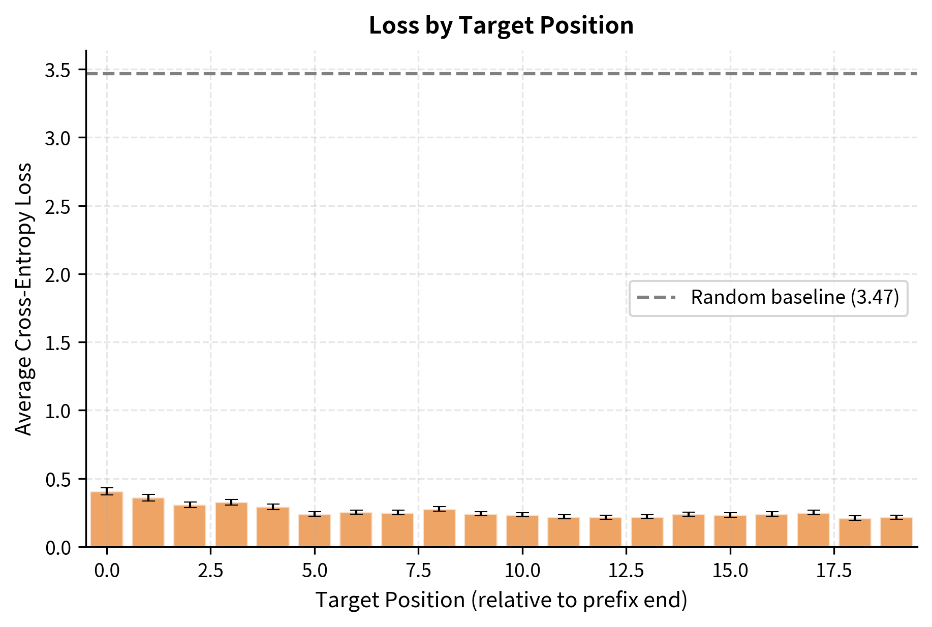
The per-position loss analysis reveals an important pattern: the first few target positions often achieve lower loss than later positions. This makes intuitive sense, the first target token has direct access to the full bidirectional prefix, while later tokens must rely increasingly on autoregressively generated context, which may be less informative than the original prefix.

Generation with Prefix LMLink Copied

Let's generate text using our trained prefix LM. The key difference from causal generation is that we start with a bidirectional prefix:

In[18]:

Code

def generate_with_prefix(
    model, prefix_text, max_new_tokens=50, temperature=0.8
):
    """Generate continuation given a prefix."""
    model.eval()

    # Encode prefix
    prefix_tokens = [char_to_idx[c] for c in prefix_text]
    prefix_len = len(prefix_tokens)
    tokens = torch.tensor(prefix_tokens).unsqueeze(0)

    with torch.no_grad():
        for _ in range(max_new_tokens):
            # Get predictions (prefix_len stays fixed, sequence grows)
            logits = model(tokens, prefix_len)

            # Sample from last position
            next_logits = logits[0, -1, :] / temperature
            probs = F.softmax(next_logits, dim=-1)
            next_token = torch.multinomial(probs, num_samples=1)

            # Append to sequence
            tokens = torch.cat([tokens, next_token.unsqueeze(0)], dim=1)

    # Decode
    generated = "".join([idx_to_char[t.item()] for t in tokens[0]])
    return generated, prefix_text

def generate_with_prefix(
    model, prefix_text, max_new_tokens=50, temperature=0.8
):
    """Generate continuation given a prefix."""
    model.eval()

    # Encode prefix
    prefix_tokens = [char_to_idx[c] for c in prefix_text]
    prefix_len = len(prefix_tokens)
    tokens = torch.tensor(prefix_tokens).unsqueeze(0)

    with torch.no_grad():
        for _ in range(max_new_tokens):
            # Get predictions (prefix_len stays fixed, sequence grows)
            logits = model(tokens, prefix_len)

            # Sample from last position
            next_logits = logits[0, -1, :] / temperature
            probs = F.softmax(next_logits, dim=-1)
            next_token = torch.multinomial(probs, num_samples=1)

            # Append to sequence
            tokens = torch.cat([tokens, next_token.unsqueeze(0)], dim=1)

    # Decode
    generated = "".join([idx_to_char[t.item()] for t in tokens[0]])
    return generated, prefix_text

Out[19]:

Console

Prefix LM Generation Examples:
--------------------------------------------------
Prefix: 'The quick'
Full: The quick urs thes thon.
A thation.
Al thatith it

Prefix: 'A journey of'
Full: A journey ofumiles a s mis d mins sinsing.
Towle win

Prefix: 'Knowledge is'
Full: Knowledge is power and knd power knd power knd k wer

The generation process treats the prefix specially: those tokens can attend to each other bidirectionally throughout generation. As new tokens are added, they see the full prefix context plus their left context, following the prefix LM pattern.

Visualizing Learned Attention PatternsLink Copied

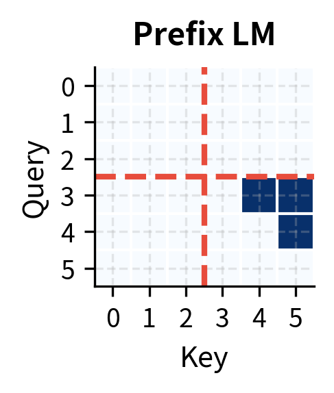
To see the prefix LM attention pattern in action, we can extract and visualize the attention weights from our trained model. This reveals how the model actually distributes attention across prefix and target positions:

Out[20]:

Visualization

Heatmap showing attention weights with strong bidirectional pattern in prefix region and causal pattern in target region. — Attention weights from the trained prefix LM model (Layer 1, Head 1). The L-shaped pattern emerges clearly: prefix positions (0-9) attend broadly to each other, while target positions (10+) focus on the prefix and their left context. Brighter colors indicate stronger attention weights.

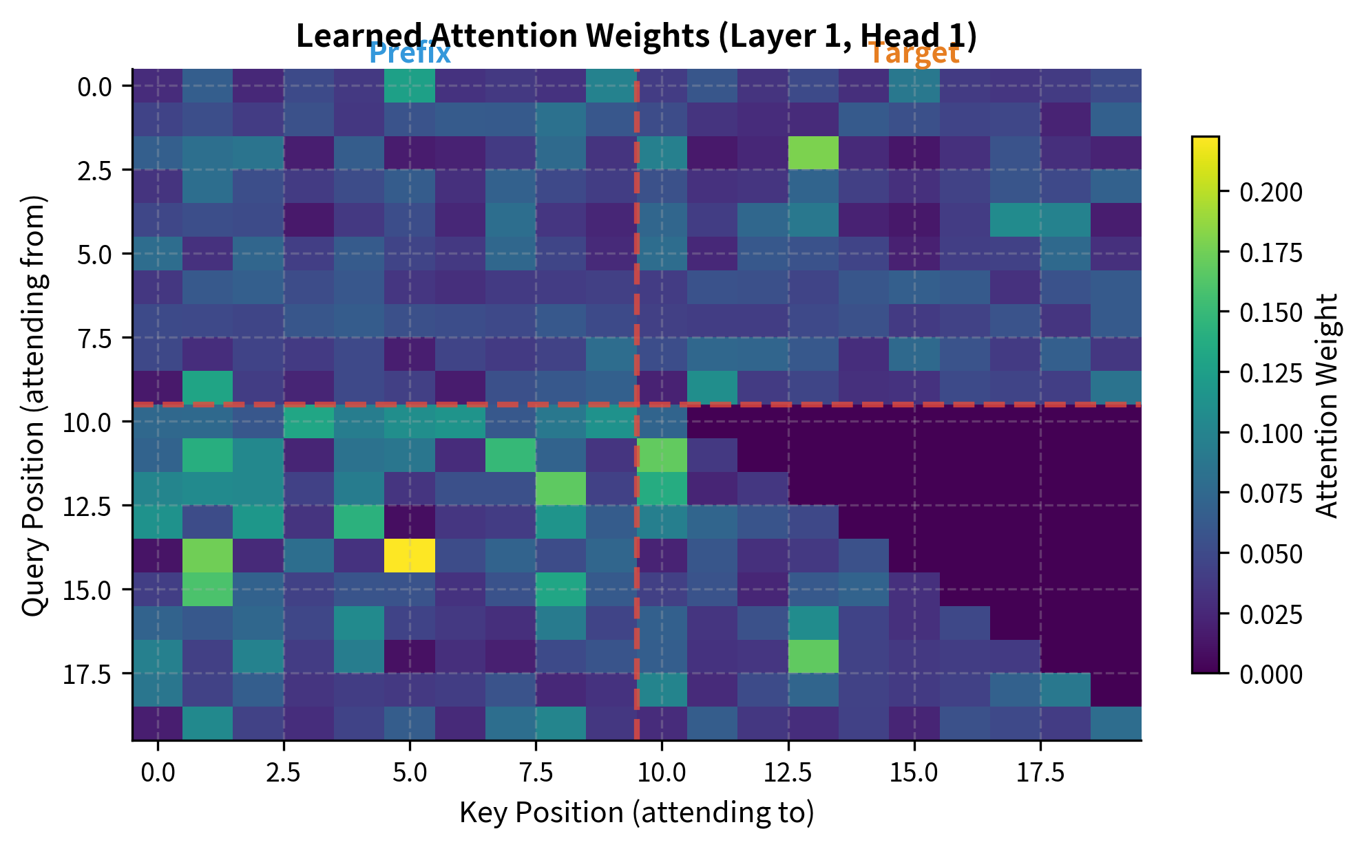
The attention heatmap reveals the prefix LM pattern in action. Notice how positions in the prefix region (left of the red dashed line) distribute attention broadly across all prefix positions, indicating bidirectional processing. Target positions (right of the line) show the characteristic causal pattern: each attends heavily to the prefix and to preceding target positions, but attention to future positions is blocked.

Out[21]:

Visualization

Bar chart showing attention distribution for a prefix position with relatively uniform weights across all positions. — Prefix position (position 5) distributes attention broadly across all positions it can see, with roughly uniform weights. This bidirectional access allows prefix tokens to incorporate context from the entire prefix.

Bar chart showing attention distribution for a target position with weights only on prefix and prior target positions. — Target position (position 15) concentrates attention on the prefix (positions 0-9) and accessible target positions (10-15), with zero weight on future positions (16+). The attention is blocked by the causal mask.

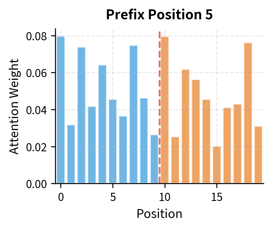
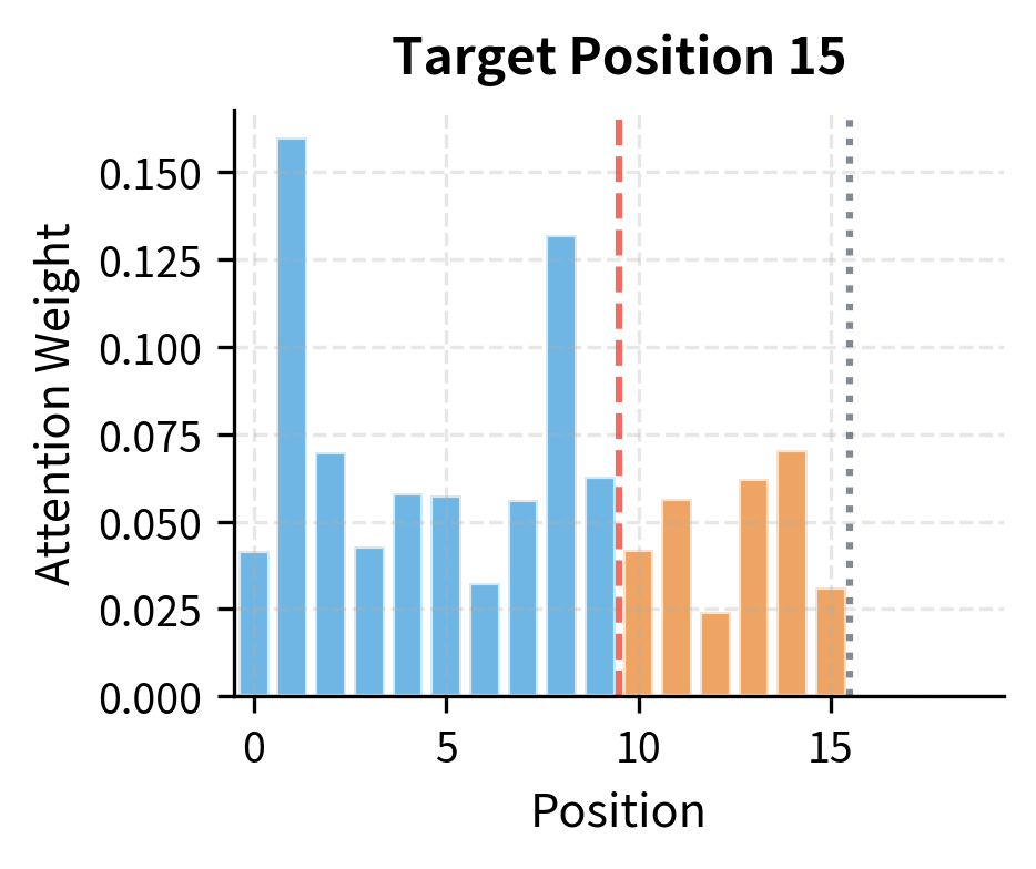
Comparing these attention distributions highlights the fundamental difference between prefix and target positions. The prefix position distributes attention across all accessible positions (itself and all others in the sequence), while the target position can only attend to the prefix and prior target positions, with future positions completely masked out.

UniLM-Style Unified TrainingLink Copied

A powerful extension of prefix LM is training a single model on multiple objectives simultaneously. UniLM (Unified Language Model) pioneered this approach, training on three objectives in each batch:

Bidirectional LM (like MLM): Full bidirectional attention, predict masked tokens
Unidirectional LM (like CLM): Causal attention, predict next token
Prefix LM: Bidirectional prefix, causal target

Out[22]:

Visualization

Full attention mask for bidirectional LM showing all positions attend to all. — Bidirectional uses full attention for understanding tasks where every position attends to every other position.

Lower triangular attention mask for unidirectional causal LM. — Unidirectional uses causal attention for generation where each position only attends to earlier positions.

L-shaped attention mask for prefix LM with bidirectional prefix and causal target. — Prefix LM combines both patterns for conditioned generation, with bidirectional prefix and causal target.

The unified training produces a model capable of all three modes. At inference time, you select the appropriate attention pattern for your task. This flexibility makes UniLM-style models particularly versatile.

In[23]:

Code

def create_unified_mask(seq_len, mode, prefix_len=None):
    """
    Create attention mask for different LM modes.

    Args:
        seq_len: Sequence length
        mode: 'bidirectional', 'unidirectional', or 'prefix'
        prefix_len: Required for 'prefix' mode

    Returns:
        Attention mask (0 = attend, -inf = block)
    """
    mask = torch.zeros(seq_len, seq_len)

    if mode == "bidirectional":
        # All attend to all
        pass

    elif mode == "unidirectional":
        # Causal masking
        for i in range(seq_len):
            for j in range(i + 1, seq_len):
                mask[i, j] = float("-inf")

    elif mode == "prefix":
        # Prefix is bidirectional, target is causal
        if prefix_len is None:
            raise ValueError("prefix_len required for prefix mode")
        for i in range(prefix_len, seq_len):
            for j in range(i + 1, seq_len):
                mask[i, j] = float("-inf")

    return mask

def create_unified_mask(seq_len, mode, prefix_len=None):
    """
    Create attention mask for different LM modes.

    Args:
        seq_len: Sequence length
        mode: 'bidirectional', 'unidirectional', or 'prefix'
        prefix_len: Required for 'prefix' mode

    Returns:
        Attention mask (0 = attend, -inf = block)
    """
    mask = torch.zeros(seq_len, seq_len)

    if mode == "bidirectional":
        # All attend to all
        pass

    elif mode == "unidirectional":
        # Causal masking
        for i in range(seq_len):
            for j in range(i + 1, seq_len):
                mask[i, j] = float("-inf")

    elif mode == "prefix":
        # Prefix is bidirectional, target is causal
        if prefix_len is None:
            raise ValueError("prefix_len required for prefix mode")
        for i in range(prefix_len, seq_len):
            for j in range(i + 1, seq_len):
                mask[i, j] = float("-inf")

    return mask

Out[24]:

Console

Unified attention masks for sequence length 6:

BIDIRECTIONAL:
  Attend positions: 36, Block positions: 0
UNIDIRECTIONAL:
  Attend positions: 21, Block positions: 15
PREFIX:
  Attend positions: 33, Block positions: 3

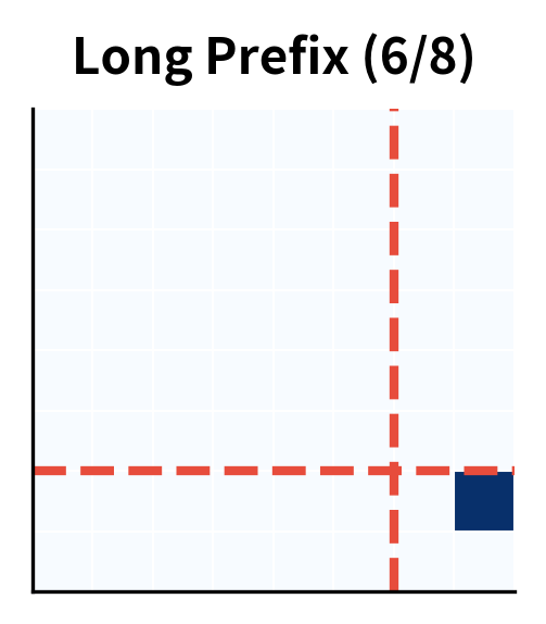
Bidirectional mode allows all 36 position pairs to attend to each other. Unidirectional mode blocks 15 positions (the upper triangle), allowing only 21 attend pairs. Prefix LM falls between these extremes: with a prefix of 3 tokens, it allows more attention than causal but less than bidirectional, as the last 3 positions still use causal masking.

Encoder-Decoder vs Decoder-Only Prefix LMLink Copied

Prefix LM can be implemented in two architectural styles, each with distinct trade-offs.

Encoder-decoder models like T5 process the prefix through a bidirectional encoder, then pass encoded representations to a causal decoder that generates the target. The encoder and decoder are separate modules with cross-attention connecting them.

Decoder-only models like GPT use a single transformer stack with the prefix LM attention mask. The same weights process both prefix and target, with the attention mask controlling information flow.

Out[25]:

Visualization

Two diagrams showing encoder-decoder and decoder-only architectures for prefix language modeling. — Two architectural approaches to prefix LM. Encoder-decoder (left) uses separate modules with cross-attention, while decoder-only (right) uses a single transformer with a hybrid attention mask. The encoder-decoder approach allows more specialization, while decoder-only is simpler and often more parameter-efficient.

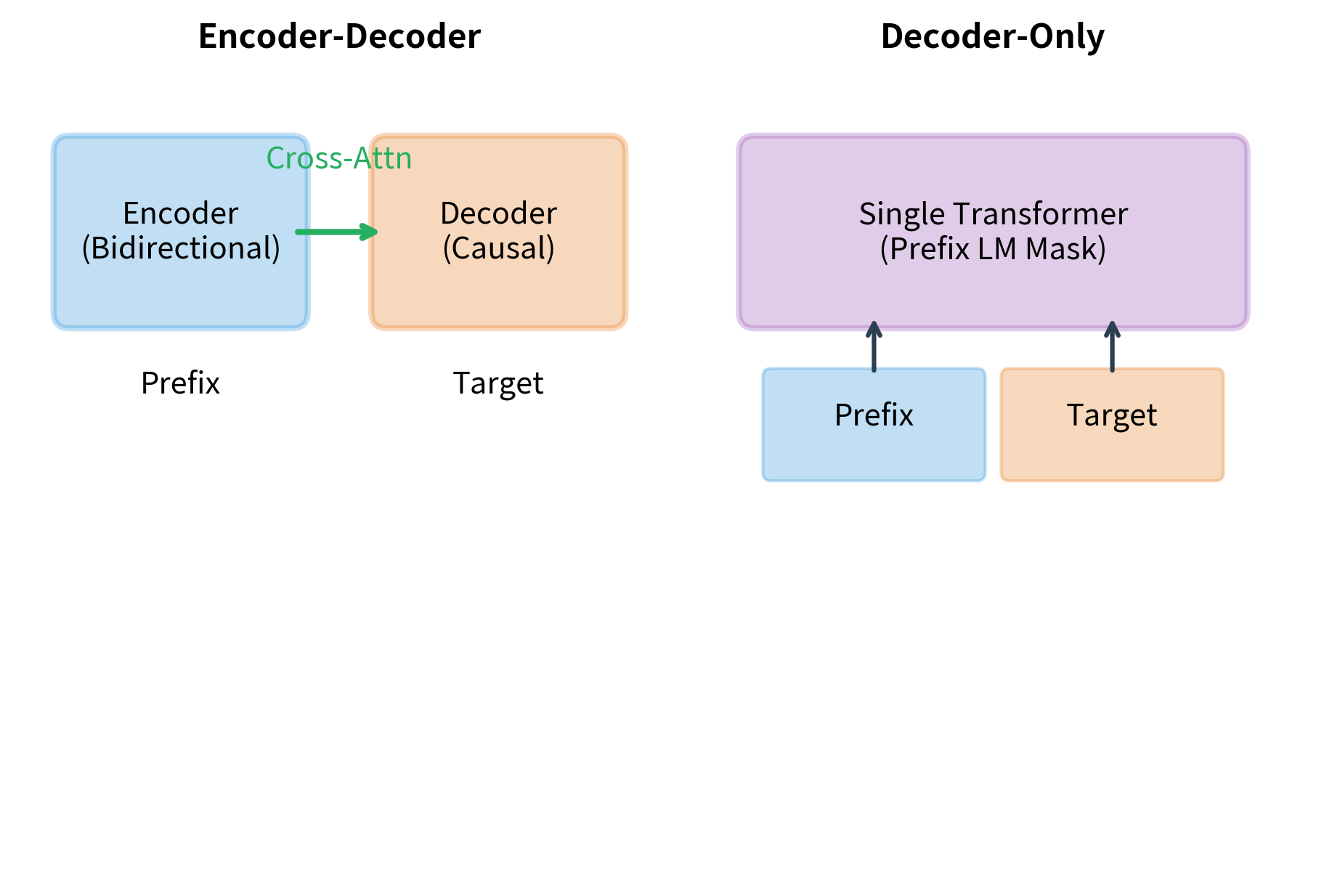
The choice between architectures depends on the application. Encoder-decoder models can process very long prefixes efficiently since encoder states are computed once and reused. Decoder-only models are simpler to implement and often perform comparably for shorter contexts.

Prefix Length and Its EffectsLink Copied

The prefix length significantly affects model behavior. Longer prefixes provide more context but leave less room for the target. The split point can be fixed or varied during training.

Out[26]:

Visualization

Attention mask with 2-token prefix showing small bidirectional region. — Short prefix (2/8): Minimal bidirectional context leaves more room for causal generation, suitable for completion tasks.

Attention mask with 4-token prefix showing balanced bidirectional and causal regions. — Medium prefix (4/8): Balanced split provides moderate context while maintaining generation flexibility.

Attention mask with 6-token prefix showing large bidirectional region. — Long prefix (6/8): Rich bidirectional context for understanding, but constrains target length, ideal for summarization.

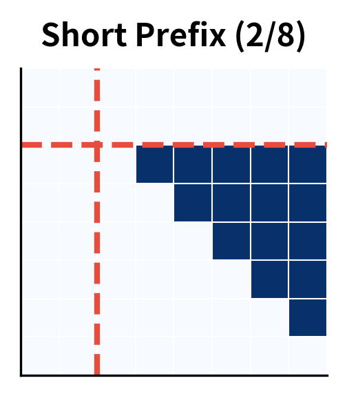
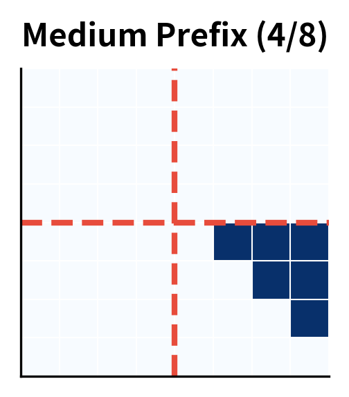
Random prefix lengths during training, as we used earlier, help the model generalize across different split points. This is especially useful for tasks where the natural prefix-target boundary varies.

Use Cases for Prefix LMLink Copied

Prefix LM naturally fits many sequence-to-sequence tasks where the input is fully known before generation begins:

Machine Translation: The source sentence is the prefix, the target sentence is the target. The full source can be processed bidirectionally, enabling the model to understand the complete meaning before generating the translation.
Summarization: Long documents form the prefix, and the concise summary is the target. Bidirectional processing of the document captures its full structure before generating a condensed version.
Question Answering: The context passage and question together form the prefix. The answer is generated as the target. The model can cross-reference question words with passage content bidirectionally.
Code Generation: Comments or specifications serve as the prefix, and the code implementation is the target. Understanding the full specification before generating code produces more coherent implementations.
Dialogue: Conversation history is the prefix, and the next response is the target. The model attends to the full conversation before generating a contextually appropriate reply.

Limitations and ImpactLink Copied

Prefix language modeling represents a principled middle ground between understanding-focused MLM and generation-focused CLM, but it introduces its own challenges.

The primary limitation is the need to define a split point. Natural language doesn't always divide cleanly into "context" and "continuation." In conversation, the boundary between prior turns and the current response is clear. In creative writing, there's no natural split. Training with random splits helps, but the model may not optimally handle all split configurations at inference time.

Computational considerations also matter. Encoder-decoder implementations can cache prefix encodings efficiently, but decoder-only implementations must recompute prefix attention as the sequence grows. For long prefixes and targets, this quadratic cost becomes significant.

Despite these challenges, prefix LM has shaped how we design language models. T5's text-to-text framework builds on prefix LM ideas, treating every NLP task as conditioned generation. UL2 (Unified Language Learner) combines prefix LM with other objectives for improved general capability. The insight that different parts of a sequence warrant different attention patterns has become a core principle in modern architecture design.

The most significant impact may be conceptual: prefix LM demonstrated that a single architecture can handle both understanding and generation by simply adjusting the attention mask. This unification has driven the field toward flexible, multi-purpose models that adapt their behavior based on how they're queried, rather than requiring separate models for separate tasks.

Key ParametersLink Copied

When training prefix language models, several parameters significantly affect performance:

prefix_len: The number of tokens in the bidirectional prefix region. Determines the split point between context and generation. Longer prefixes provide richer context but leave less room for target generation.
min_prefix_frac / max_prefix_frac: When using random prefix lengths during training (0.3 to 0.7 in our example), these control the range of possible split points. Wider ranges help the model generalize across different prefix-target ratios.
d_model: The hidden dimension of the transformer. Larger values (64, 128, 256) increase model capacity for capturing complex patterns in both prefix and target.
n_heads: Number of attention heads. More heads allow the model to attend to different aspects of the prefix context simultaneously.
n_layers: Depth of the transformer stack. Deeper models can learn more complex relationships between prefix context and target generation.
learning_rate: Typically 1e-4 to 1e-3 for prefix LM training. The bidirectional prefix may allow slightly higher learning rates than pure causal LM since gradients flow more freely.
temperature: Controls randomness during generation (0.7 to 1.0 typical). Lower values make generation more deterministic, higher values increase diversity.

SummaryLink Copied

Prefix language modeling combines bidirectional context encoding with causal generation, offering a powerful middle ground between MLM and CLM. This chapter covered the key concepts:

The prefix LM split divides sequences into a bidirectional prefix and a causal target, enabling rich context understanding while maintaining generation capability
The attention pattern forms an L-shape, with full attention in the prefix region and causal masking in the target region
Loss computation focuses only on target positions, training the model specifically for conditioned generation
UniLM-style training combines multiple objectives (bidirectional, causal, prefix) in a single model, creating versatile architectures
Architectural choices include encoder-decoder and decoder-only implementations, each with distinct trade-offs for different use cases
Applications span translation, summarization, QA, and dialogue, where the prefix-target structure matches the task naturally

The next chapter explores replaced token detection, an alternative to masking that uses a discriminative objective for more efficient pretraining.

QuizLink Copied

Ready to test your understanding? Take this quick quiz to reinforce what you've learned about prefix language modeling.

Loading component...

Track your reading progress

Sign in to mark chapters as read and track your learning journey

Sign in →

Comments

Back to Language AI Handbook

Previous Chapter

Span Corruption

Next Chapter

Replaced Token Detection

Reference

BIBTEXAcademic

@misc{prefixlanguagemodelingcombiningbidirectionalcontextwithcausalgeneration, author = {Michael Brenndoerfer}, title = {Prefix Language Modeling: Combining Bidirectional Context with Causal Generation}, year = {2025}, url = {https://mbrenndoerfer.com/writing/prefix-language-modeling-bidirectional-causal-generation}, organization = {mbrenndoerfer.com}, note = {Accessed: 2025-12-19} }

APAAcademic

Michael Brenndoerfer (2025). Prefix Language Modeling: Combining Bidirectional Context with Causal Generation. Retrieved from https://mbrenndoerfer.com/writing/prefix-language-modeling-bidirectional-causal-generation

MLAAcademic

Michael Brenndoerfer. "Prefix Language Modeling: Combining Bidirectional Context with Causal Generation." 2025. Web. 12/19/2025. <https://mbrenndoerfer.com/writing/prefix-language-modeling-bidirectional-causal-generation>.

CHICAGOAcademic

Michael Brenndoerfer. "Prefix Language Modeling: Combining Bidirectional Context with Causal Generation." Accessed 12/19/2025. https://mbrenndoerfer.com/writing/prefix-language-modeling-bidirectional-causal-generation.

HARVARDAcademic

Michael Brenndoerfer (2025) 'Prefix Language Modeling: Combining Bidirectional Context with Causal Generation'. Available at: https://mbrenndoerfer.com/writing/prefix-language-modeling-bidirectional-causal-generation (Accessed: 12/19/2025).

SimpleBasic

Michael Brenndoerfer (2025). Prefix Language Modeling: Combining Bidirectional Context with Causal Generation. https://mbrenndoerfer.com/writing/prefix-language-modeling-bidirectional-causal-generation

Direct link:

https://mbrenndoerfer.com/writing/prefix-language-modeling-bidirectional-causal-generation

About the author: Michael Brenndoerfer

All opinions expressed here are my own and do not reflect the views of my employer.

Michael currently works as an Associate Director of Data Science at EQT Partners in Singapore, leading AI and data initiatives across private capital investments.

With over a decade of experience spanning private equity, management consulting, and software engineering, he specializes in building and scaling analytics capabilities from the ground up. He has published research in leading AI conferences and holds expertise in machine learning, natural language processing, and value creation through data.

View Full Resume Publications Contact Books

Prefix Language Modeling: Combining Bidirectional Context with Causal Generation

Prefix Language ModelingLink Copied

The Prefix LM IntuitionLink Copied

The Prefix LM ObjectiveLink Copied

From Intuition to FormalizationLink Copied

The Mathematical FormulationLink Copied

Understanding the ConditioningLink Copied

Why Loss on Target Only?Link Copied

The Prefix LM Attention PatternLink Copied

Anatomy of the Attention MaskLink Copied

Implementing the MaskLink Copied

Comparing Attention PatternsLink Copied

Implementing Prefix LM TrainingLink Copied

The Attention MechanismLink Copied

The Complete ModelLink Copied

Training on Prefix-Target PairsLink Copied

Preparing the DataLink Copied

The Training Loop with Random SplitsLink Copied

Generation with Prefix LMLink Copied

Visualizing Learned Attention PatternsLink Copied

UniLM-Style Unified TrainingLink Copied

Encoder-Decoder vs Decoder-Only Prefix LMLink Copied

Prefix Length and Its EffectsLink Copied

Use Cases for Prefix LMLink Copied

Limitations and ImpactLink Copied

Key ParametersLink Copied

SummaryLink Copied

QuizLink Copied

Comments

Reference

About the author: Michael Brenndoerfer

Related Content

Denoising Objectives: BART's Corruption Strategies for Language Models

Replaced Token Detection: ELECTRA's Efficient Pretraining Objective

Span Corruption: T5's Pretraining Objective for Sequence-to-Sequence Learning

Stay updated