

Learn how sliding window attention reduces transformer complexity from quadratic to linear by restricting attention to local neighborhoods, enabling efficient processing of long documents.

This article is part of the free-to-read Language AI Handbook
Choose your expertise level to adjust how many terms are explained. Beginners see more tooltips, experts see fewer to maintain reading flow. Hover over underlined terms for instant definitions.
Sliding Window Attention
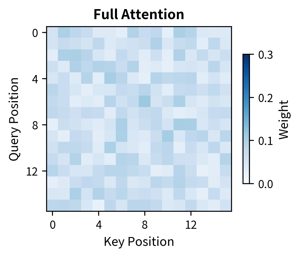
Standard attention computes all pairwise interactions between tokens, but most of that computation may be wasted. In natural language, context is often local: the meaning of a word depends heavily on its immediate neighbors. Consider the phrase "the quick brown fox jumps over the lazy dog." When determining what "jumps" means, the model needs "fox" (the subject) and "over" (what follows), but distant tokens like "the" or "dog" contribute less to understanding this particular word. Sliding window attention exploits this locality by restricting each token to attend only to tokens within a fixed-size window around it.
This chapter explores how sliding window attention works, why it reduces complexity from quadratic to linear, and how to implement it effectively. We will also examine the trade-offs: what do we lose when tokens cannot see beyond their local window, and how can we address these limitations?
The Locality Assumption
Before diving into the mechanics, let's understand why local attention makes sense. Natural language exhibits strong locality: adjacent words form phrases, phrases form clauses, and meaning often crystallizes within a narrow span.
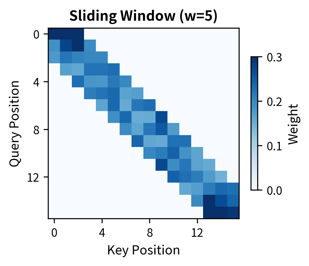
Sliding window attention restricts each token to attending only to tokens within a fixed distance (the window size). Instead of attention weights, we compute approximately weights, achieving linear complexity in sequence length.
Consider how you read this sentence. When your eye lands on "read," you immediately connect it to "you" (subject) and "this sentence" (object), all within a few tokens. You do not need to re-read the beginning of the paragraph to understand this verb. Sliding window attention captures this intuition by limiting attention to a local neighborhood.
The key insight is that attention patterns in trained transformers often concentrate locally. Research analyzing attention weights in models like BERT and GPT-2 found that many heads allocate most attention mass to nearby tokens. By building this locality bias into the architecture, we can dramatically reduce computation while preserving much of the model's representational power.
How Sliding Window Attention Works
To understand sliding window attention, we need to answer three questions: What does "local" mean mathematically? How do we enforce locality in the attention computation? And how does this change the algorithm's behavior? Let's build up the formalism step by step, starting from the intuition and arriving at a complete mathematical specification.
From Intuition to Neighborhoods
In standard attention, every token can attend to every other token. This creates a fully connected graph where information flows freely between all positions. But we observed that most meaningful connections occur between nearby tokens. The first step toward efficiency is formalizing what "nearby" means.
Consider token in a sequence. Which tokens should it attend to? The natural answer is: tokens within some fixed distance. If we set a window size , we want token to attend only to tokens that are close enough. We measure closeness by position distance:
where:
- : the position of the query token (the one computing its representation)
- : the position of the key token (a candidate for attention)
- : the window size (total number of positions each token can attend to)
- : the absolute distance between the two positions
- : half the window size (rounded down), giving the maximum distance in each direction
This formula defines a neighborhood around each token. With , token at position 10 can attend to positions 8, 9, 10, 11, and 12. The neighborhood extends positions in each direction, plus the token itself. Token at position 3 can attend to positions 1, 2, 3, 4, and 5. Every token has the same sized window, centered on itself.
Why floor instead of exact division? Window sizes are typically odd (like 3, 5, or 257) so the token sits exactly in the middle. For even windows, the floor gives a slight asymmetry, attending to one more position on one side than the other. This rarely matters in practice.
Translating Neighborhoods into Masks
Now we face a practical question: how do we tell the attention mechanism which positions each token should attend to? Standard attention computes a score between every query-key pair. We need a way to "zero out" the scores for positions outside the neighborhood.
The solution is an attention mask: a matrix that modifies the raw attention scores before softmax. The mask acts like a filter, allowing some connections and blocking others. For each pair of positions , we assign a mask value:
where:
- : the mask value at position
- : no modification (allow attention)
- : block this connection entirely
Why these particular values? The mask gets added to the raw attention scores before softmax. Adding 0 leaves the score unchanged, preserving normal attention behavior for positions within the window. Adding ensures that after the exponential in softmax, the weight becomes exactly 0:
The blocked position contributes nothing to the output. In implementation, we use a large negative number like rather than true infinity to avoid numerical issues, but the effect is identical.
The Complete Attention Formula
With the mask defined, we can write the full sliding window attention computation. Start with the standard attention formula:
This computes scores between all query-key pairs (), normalizes them into weights (softmax), and uses those weights to aggregate values. Sliding window attention inserts the mask before softmax:
where:
- : the query matrix, with one row per token
- : the key matrix, with one row per token
- : the value matrix, containing information to aggregate
- : the sliding window mask
- : the raw attention scores before masking
- : the dimension of query and key vectors
- : scaling factor to prevent dot products from growing too large
The computation proceeds in four steps:
- Compute raw scores: Multiply queries by keys to get scores
- Apply mask: Add to block positions outside each token's window
- Normalize: Apply softmax row-wise to convert scores to weights
- Aggregate: Multiply weights by values to get the output
After masking and softmax, each row of the weight matrix sums to 1, but the non-zero weights are concentrated in a band around the diagonal. Token 5 has non-zero weights only for tokens 3-7 (with ). Token 100 has non-zero weights only for tokens 98-102. The sparse pattern emerges from the mask, even though we computed all scores.
Window Patterns
Several window configurations are possible. The most common is the symmetric window where each token looks an equal distance forward and backward:
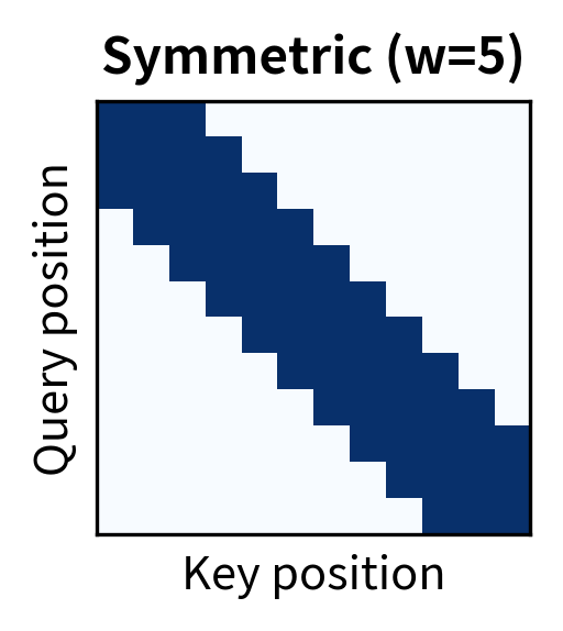
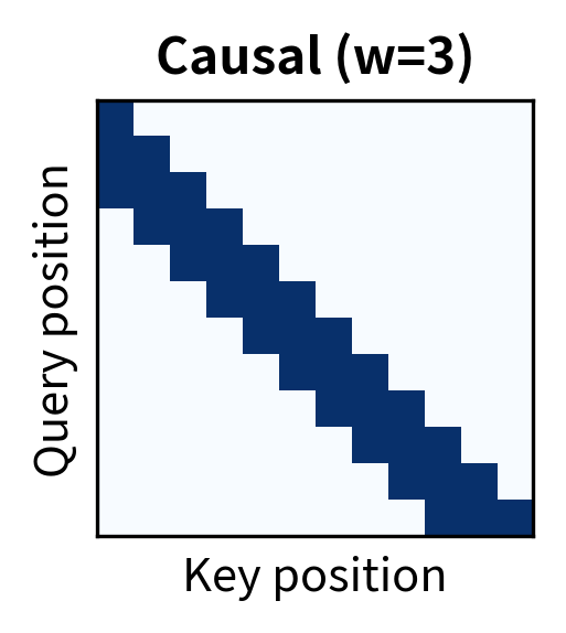
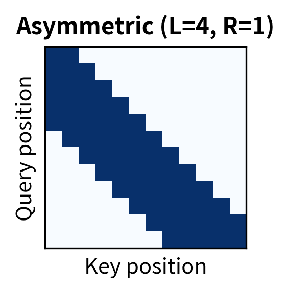
The symmetric window suits bidirectional models like BERT where context flows in both directions. The causal window is essential for autoregressive models like GPT, where tokens must not attend to future positions. Asymmetric windows can be useful when past context is more informative than future context, or vice versa.
Complexity Analysis
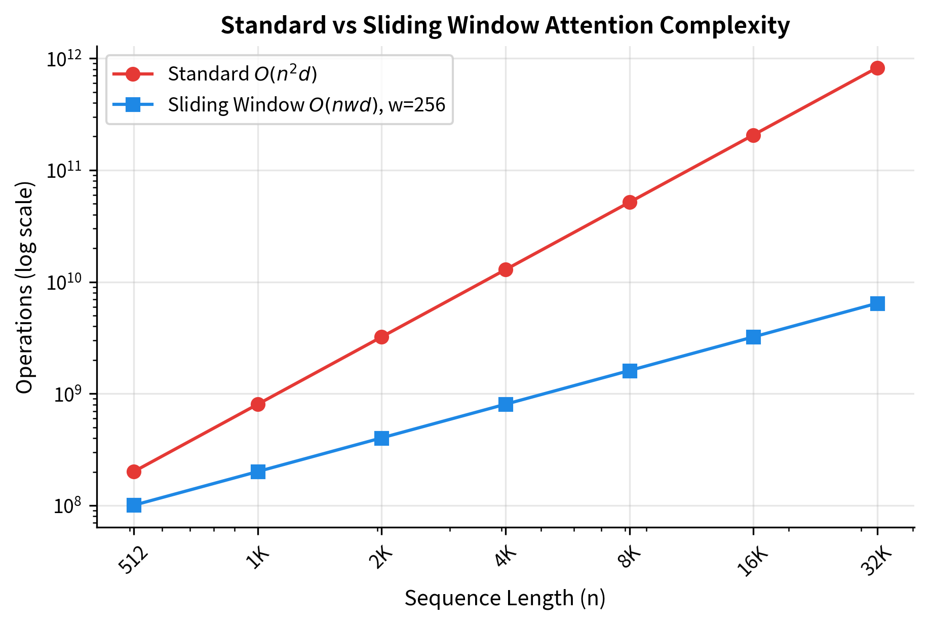
Understanding the complexity reduction is key to appreciating why sliding window attention matters. Standard attention computes attention scores because every token attends to every other token. With a sliding window of size , each token attends to at most positions, yielding approximately attention scores instead.
The critical insight is that is a fixed constant (typically 128-512), independent of sequence length. This transforms the complexity:
where:
- : sequence length (the variable that grows with input size)
- : window size (a fixed hyperparameter, constant with respect to )
- : model dimension (also fixed for a given model architecture)
Since both and are constants for a given model, the complexity is linear in . This linear scaling means we can process sequences of arbitrary length with proportional, rather than quadratic, cost. A 10x longer sequence requires only 10x more computation, not 100x.
The speedup grows linearly with sequence length. At 512 tokens, sliding window provides a 2x speedup. At 16K tokens, the speedup reaches 64x. This difference becomes crucial for processing long documents, where standard attention would be prohibitively expensive.
Window Size Selection
Choosing the right window size involves balancing efficiency against the ability to capture dependencies. Smaller windows are faster but may miss important long-range relationships. Larger windows capture more context but reduce the computational advantage.
Factors Influencing Window Size
Several considerations guide window size selection:
-
Task requirements: Classification tasks often need only local features, while question answering may require longer-range reasoning. Summarization tasks might need to connect information across paragraphs.
-
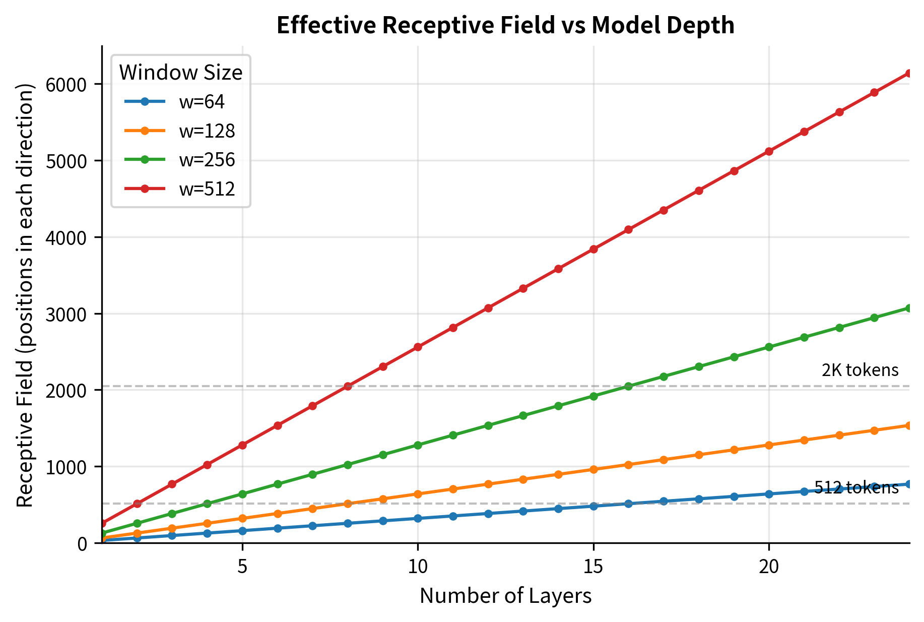
Model depth: With multiple layers, information can propagate across the sequence. In a model with layers and window size , information can theoretically travel positions in each direction through the network. This is because each layer allows a token to gather information from positions on each side, and stacking layers compounds this reach. A 12-layer model with window size 128 can propagate information across positions in each direction.
-
Computational budget: Larger windows cost more. If latency is critical, smaller windows enable faster inference.
-
Sequence length: The ratio of window size to sequence length matters. A 256-token window covers an 8K-token document poorly but might suffice for 1K-token inputs.
Empirical Guidance
Research on efficient transformers has explored various window sizes:
- Longformer: Uses window sizes of 256-512 tokens, combined with global attention on specific positions
- BigBird: Employs block sizes of 64 tokens with random and global attention patterns
- Mistral 7B: Uses a 4,096-token sliding window, covering substantial context for most applications
A useful heuristic is to start with a window size that captures typical sentence or paragraph lengths (128-512 tokens) and increase it if downstream task performance suffers.
The receptive field table shows how layer depth compensates for narrow windows. A 64-token window in a 24-layer model allows information to propagate 768 positions, while the same window in a 6-layer model reaches only 192 positions. This explains why deeper models can often use smaller windows without sacrificing performance.
Dilated Sliding Windows
Standard sliding windows have a limitation: the receptive field grows slowly with window size. To see positions 100 tokens away, you need either a window of 200 tokens (expensive) or many layers for information to propagate (slow). Dilated sliding windows offer a third option: spread the attention across a wider range by skipping intermediate positions.
Dilated sliding window attention attends to positions at regular intervals (the dilation rate) rather than consecutive positions. This expands the effective receptive field while keeping the number of attended positions constant.
The intuition comes from signal processing and computer vision. A dilated convolution samples every th position instead of consecutive positions, covering more ground with the same number of parameters. Dilated attention applies the same principle: instead of attending to your 5 nearest neighbors, attend to 5 positions spaced 2 apart.
How Dilation Works
Let's formalize this idea. In standard attention, the attended positions form a consecutive sequence centered on the query. With dilation, we introduce gaps between attended positions.
With dilation rate and attended positions, token attends to the following set of positions:
where:
- : the query position (the token computing its attention)
- : the dilation rate (the gap between consecutive attended positions)
- : the number of positions to attend to (same as in non-dilated attention)
- : the number of positions on each side of the center
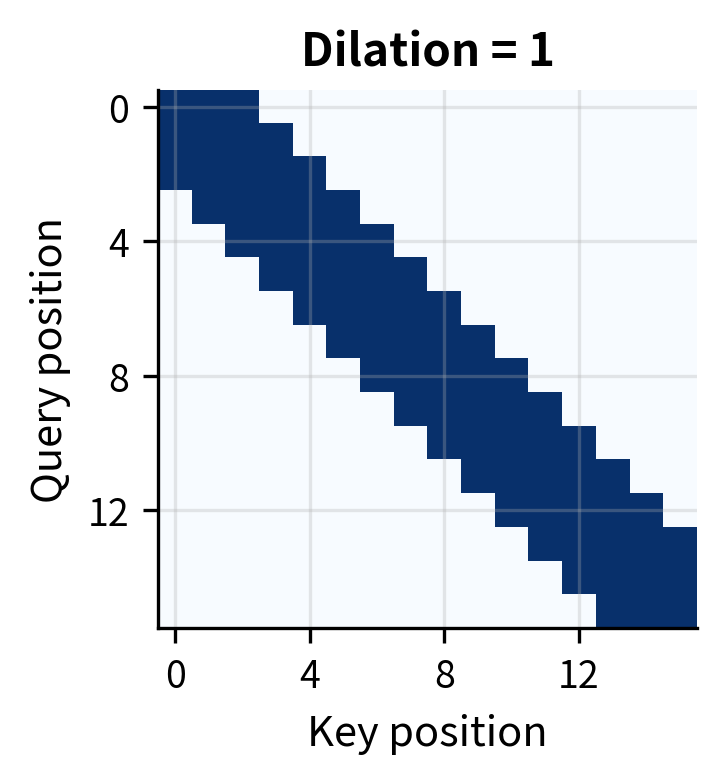
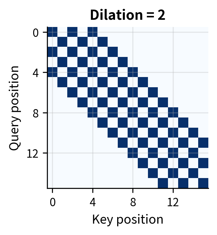
The dilation rate acts as a multiplier on the offset from the center position. With (no dilation), we get the standard consecutive window. With , we skip every other position, doubling the effective range while attending to the same number of positions.
For example, with and , token at position 10 attends to positions rather than the consecutive window . Both patterns attend to exactly 5 positions, but the dilated version covers a range of 8 positions instead of 4.
Multi-Scale Attention with Varying Dilation
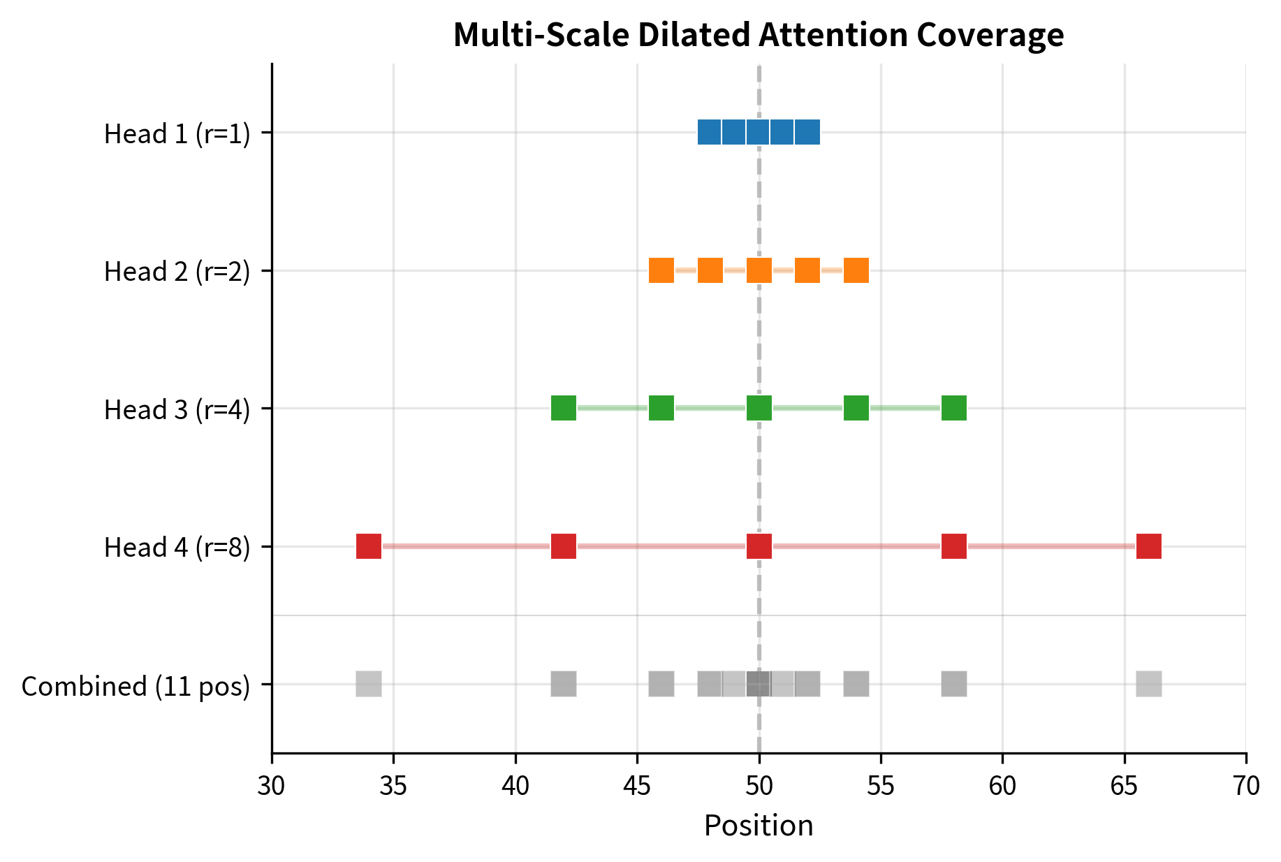
A single dilation rate creates gaps in coverage: with , we miss all odd-positioned tokens. The solution is to use different dilation rates across attention heads. Some heads use for fine-grained local attention, others use for medium-range context, and still others use or for long-range dependencies.
This multi-scale approach, used in models like Longformer, creates a powerful combination. The union of all heads covers a broad range of positions, each head specializes in a particular scale, and the total computation remains sparse. Think of it like having multiple photographers at an event: one captures close-ups, another medium shots, and a third wide angles. Together, they document everything without any single photographer doing all the work.
The multi-scale approach extends the effective receptive field while maintaining sparse attention. With dilation rates of and 5 positions per head, the model covers a range of 32 positions with 11 unique attention connections, achieving both broad coverage and computational efficiency.
Implementation
With the theory established, let's translate these ideas into working code. We'll build sliding window attention step by step, starting with the most straightforward approach and progressively optimizing. Along the way, you'll see how the mathematical formulas map directly to implementation choices.
Mask-Based Implementation
The most direct implementation follows the formula exactly: compute all attention scores, apply the mask, run softmax, and aggregate values. This approach prioritizes clarity over efficiency, making it ideal for understanding the mechanism.
First, we need helper functions. The softmax function normalizes scores into probability distributions. We implement a numerically stable version that subtracts the maximum before exponentiating to prevent overflow:
The mask creation function iterates through each position and sets the mask to 0 for positions within the window, for positions outside. Notice how the code directly implements our mathematical definition: for symmetric windows, we check if the distance is at most half_window; for causal windows, we also require that the key position is not in the future.
This implementation explicitly constructs the full mask, which works well for moderate sequence lengths. For very long sequences, we'll need a more efficient approach, but this version is perfect for understanding the pattern.
With the mask function ready, we can implement the complete attention computation:
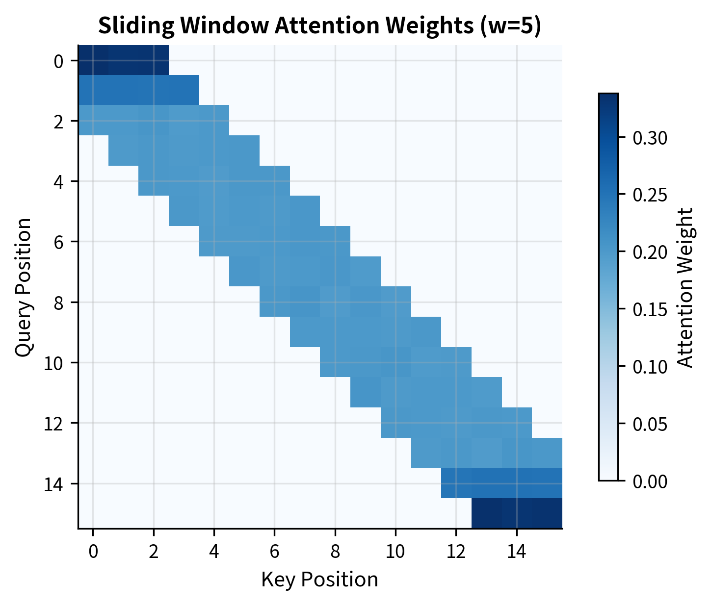
This function follows our four-step process exactly: compute scores (), scale by , add the mask, apply softmax, and multiply by values. The function returns both the output and the attention weights, which we'll visualize to verify the windowed pattern.
Let's test this implementation with a concrete example. We'll create random queries, keys, and values, then examine the attention pattern:
The attention weights confirm that token 8 attends only to positions 6-10 (a window of 5 centered on position 8), with all other weights effectively zero.
Efficient Block-Based Implementation
The mask-based implementation has a problem: it still computes and stores the full attention matrix, even though most entries are zero. For a 10,000-token sequence, we'd allocate 100 million floats just for the attention weights. This defeats the purpose of sliding window attention.
The solution is to never materialize the full matrix. Instead, we process each position independently, computing attention only over its local window. This insight transforms memory complexity from to , where is the window size:
The key insight is in the loop body. For each position , we compute the window boundaries, extract only the relevant keys and values, compute attention scores over just positions, and aggregate. Each iteration uses memory instead of , and we never store the full attention matrix.
This approach trades sequential processing for memory efficiency. In practice, production implementations use batched operations and GPU-optimized kernels to process multiple positions in parallel while still avoiding the full matrix.
Let's verify that both implementations produce identical results:
The negligible difference (on the order of ) confirms that both implementations compute identical results. The efficient version achieves the same output while using significantly less memory for long sequences.
Causal Sliding Window for Language Models
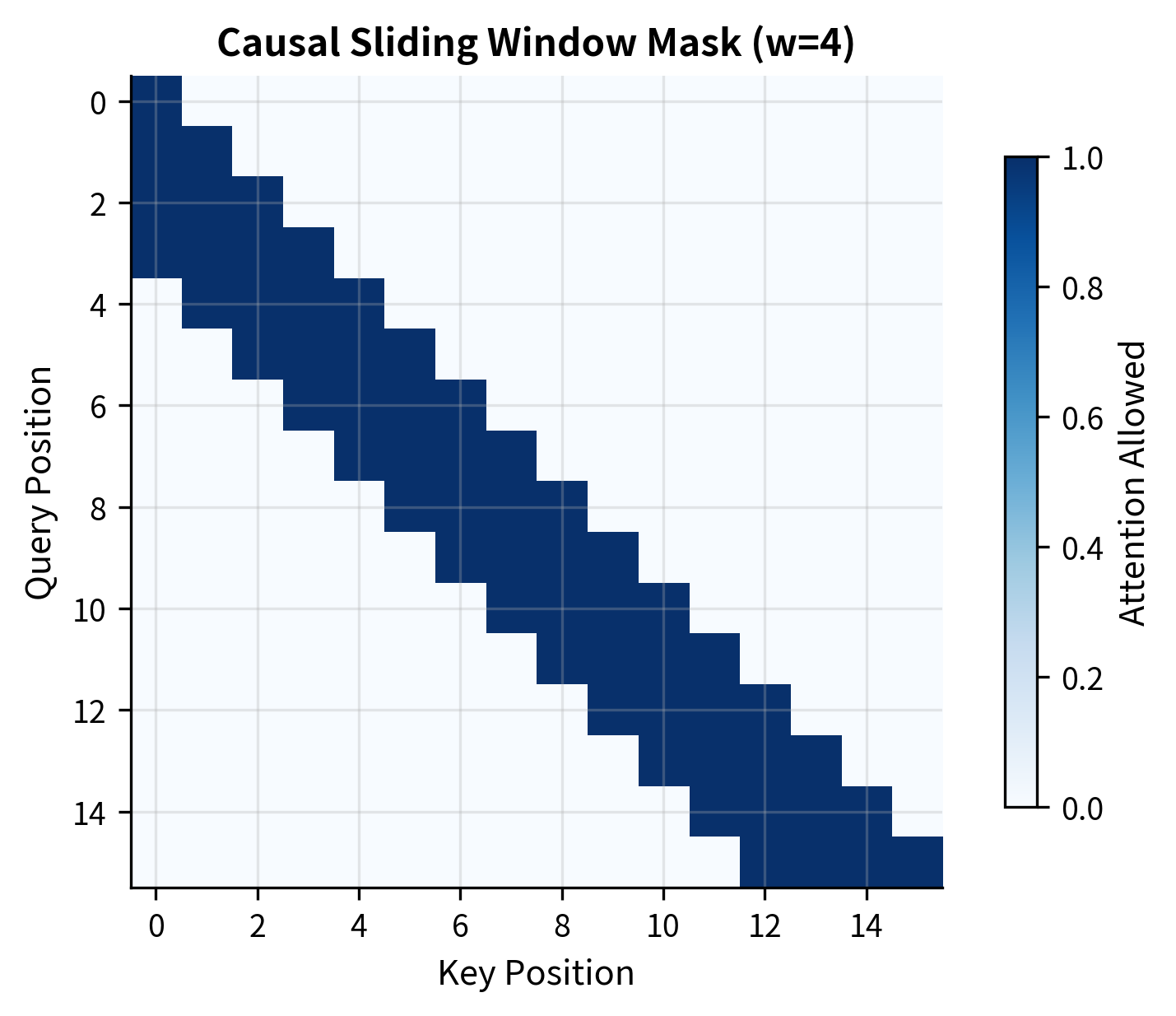
For autoregressive language models like GPT, we need an additional constraint: tokens must not attend to future positions. If token 10 could see token 11, it would be "cheating" during text generation, looking at words it's supposed to predict.
Combining causality with sliding windows creates a pattern where each token sees at most previous tokens, including itself. The window is asymmetric: all context comes from the past. Token 10 with attends to tokens 7, 8, 9, and 10, never tokens 11 and beyond:
Mistral-Style Windowed Attention
Mistral 7B popularized sliding window attention in modern large language models. Their approach uses a 4,096-token window size, which covers most practical context lengths while enabling efficient inference.
Key Design Choices
Mistral's implementation incorporates several practical considerations:
- Large window size (4096): Covers entire documents in many use cases, reducing the need for global tokens
- Rolling buffer KV cache: During generation, only the most recent key-value pairs are stored
- Pre-fill and chunking: Long prompts are processed in chunks to manage memory
The rolling buffer approach is particularly elegant. Traditional transformers store all past key-value pairs, requiring memory that grows with sequence length:
where:
- : memory required for the full KV cache
- : current sequence length (grows during generation)
- : number of transformer layers
- : model dimension
With sliding window attention, we only store the most recent key-value pairs, giving constant memory usage:
where is the window size. Since , , and are all constants for a given model, memory usage becomes independent of sequence length. This is the key insight that enables generating arbitrarily long sequences without running out of memory.
After adding 6 tokens to a cache with window size 4, tokens 0 and 1 have been evicted. The cache now contains only tokens 2, 3, 4, and 5, demonstrating how the circular buffer automatically discards the oldest entries when it reaches capacity. This behavior mirrors what happens during autoregressive generation in models like Mistral.
Memory Comparison
The rolling buffer approach provides substantial memory savings for long sequences:
The memory comparison reveals the scaling advantage of the rolling buffer. At 1,024 tokens (below the window size), both approaches use the same memory. At 4,096 tokens (exactly the window size), they remain equivalent. Beyond that point, the savings become dramatic: at 16K tokens, the rolling buffer uses 75% less memory, and at 64K tokens, savings reach over 93%.
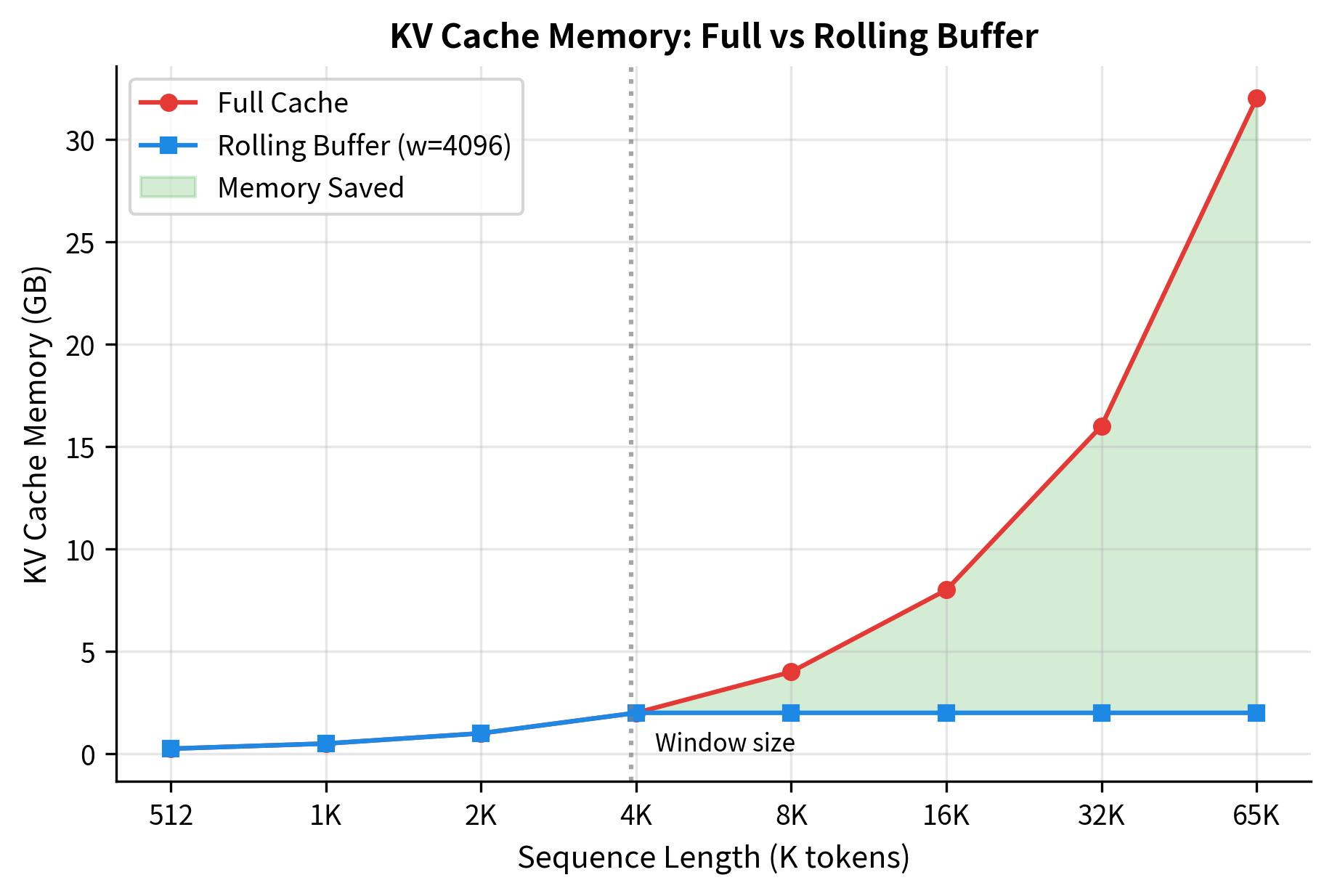
This enables processing long documents on hardware that could not otherwise accommodate them.
Limitations and Impact
Sliding window attention achieves linear complexity by making a fundamental trade-off: tokens beyond the window cannot directly attend to each other. This creates important limitations that you must consider when deploying these models.
The most significant challenge is capturing long-range dependencies. Consider a question-answering task where the answer appears at the beginning of a long document and the question at the end. With a window of 512 tokens and a document of 10,000 tokens, direct attention between question and answer is impossible. Information must propagate through intermediate layers, potentially degrading or losing signal along the way. Experiments have shown that sliding window models perform well on tasks where relevant context is local but struggle when important information spans large distances.
Another limitation relates to positional awareness. Standard transformers with full attention can learn to recognize absolute positions through attention patterns. With sliding window attention, each token sees the same local structure regardless of its absolute position in the sequence. While positional embeddings help, some tasks that require precise long-range position tracking may suffer.
Despite these limitations, sliding window attention has proven remarkably effective in practice. Modern language models like Mistral combine it with large windows (4,096 tokens) that cover most practical contexts. For document understanding, the combination of sliding windows with global attention tokens (covered in the next chapter) addresses most long-range needs while maintaining efficiency. The approach has enabled scaling to context lengths that would be impractical with full attention, opening new applications in document processing, code analysis, and long-form text generation.
The practical impact extends beyond computational savings. Standard attention requires storing the full attention matrix, giving memory complexity. Sliding window attention stores only the non-zero entries within each window, reducing memory to . Since is constant, this is effectively linear in sequence length. A model with full attention at 16K tokens might require a high-end GPU, while the same model with sliding window attention can run on modest hardware. This democratization of long-context processing has accelerated both research and deployment of language models for real-world applications.
Summary
Sliding window attention addresses the quadratic complexity of standard attention by restricting each token to attend only within a local window. The core ideas and takeaways from this chapter:
-
Linear complexity: By attending to a fixed window of positions, complexity drops from to , enabling efficient processing of long sequences.
-
Window patterns: Symmetric windows work for bidirectional models, while causal windows suit autoregressive generation. Asymmetric and dilated windows offer additional flexibility.
-
Effective receptive field: Through multiple layers, information propagates beyond the immediate window. A model with layers and window has an effective receptive field of approximately positions in each direction, allowing distant tokens to influence each other indirectly.
-
Implementation efficiency: Memory-efficient implementations avoid materializing the full attention matrix, instead computing attention block by block.
-
Rolling KV cache: For autoregressive generation, a circular buffer stores only the most recent key-value pairs, providing constant memory usage regardless of sequence length.
-
Trade-offs: The locality assumption sacrifices direct long-range attention. Tasks requiring connections across distant positions may need additional mechanisms like global attention tokens.
-
Practical success: Models like Mistral demonstrate that sliding window attention with large windows (4,096+ tokens) provides excellent performance on most tasks while enabling efficient inference.
The next chapter explores global attention tokens, which complement sliding window attention by providing a mechanism for information to flow across the entire sequence, combining the efficiency of local attention with the expressiveness of global connectivity.
Key Parameters
When implementing or configuring sliding window attention, several parameters directly impact both performance and computational efficiency:
-
window_size: The number of positions each token can attend to. Larger windows capture more context but increase computation. Common values range from 128-512 for efficient models to 4,096 for models like Mistral. Choose based on the expected range of relevant dependencies in your task.
-
causal: Whether to use causal masking (True for autoregressive language models, False for bidirectional models like BERT). Causal masking ensures tokens cannot attend to future positions, which is required for text generation.
-
dilation_rate: For dilated sliding windows, controls the gap between attended positions. A rate of 1 gives standard consecutive attention; rate 2 skips every other position, doubling the effective range. Use multiple dilation rates across heads for multi-scale attention.
-
num_layers: The number of transformer layers affects the effective receptive field. With layers and window , information can propagate approximately positions in each direction. Deeper models can use smaller windows.
-
d_k / d_head: The dimension of query and key vectors. Standard values follow where is the number of heads. This affects the scaling factor in attention score computation.
-
dtype_bytes: Memory precision for KV cache storage. Use 2 bytes for fp16/bf16 (recommended) or 4 bytes for fp32. Half precision halves memory usage with negligible quality impact.
Quiz
Ready to test your understanding? Take this quick quiz to reinforce what you've learned about sliding window attention and its efficiency benefits.

Comments