

Learn how BigBird combines sliding window, global tokens, and random attention to achieve O(n) complexity while maintaining theoretical guarantees for long document processing.

This article is part of the free-to-read Language AI Handbook
Choose your expertise level to adjust how many terms are explained. Beginners see more tooltips, experts see fewer to maintain reading flow. Hover over underlined terms for instant definitions.
BigBird
Standard transformers struggle with long documents because their attention mechanism scales quadratically with sequence length. For a sequence of tokens, full self-attention computes attention scores, meaning a 4,096-token document requires computing and storing over 16 million scores (). This quickly exhausts GPU memory. BigBird addresses this bottleneck by combining three complementary attention patterns: sliding window attention for local context, global tokens for long-range communication, and random attention for efficient graph connectivity. This hybrid approach reduces complexity from to while preserving the model's ability to reason over entire documents.
What makes BigBird particularly significant is not just its practical efficiency, but its theoretical foundation. The authors proved that their sparse attention pattern can approximate any full attention function, and crucially, that the random attention component makes the pattern a universal approximator of sequence-to-sequence functions. This chapter explores the BigBird attention pattern, the mathematical justification for random connections, and how this architecture compares to Longformer and other sparse attention approaches.
The BigBird Attention Pattern
To understand BigBird, we need to ask a fundamental question: what does each token actually need to see? Full self-attention assumes every token might need information from every other token, leading to the bottleneck. But this assumption is wasteful. In practice, tokens draw information from three distinct sources: their immediate neighbors (for local syntax and semantics), a few special positions that summarize global context, and occasionally, distant positions that happen to be relevant. BigBird formalizes this intuition into three complementary attention components.
BigBird attention is a sparse attention mechanism that combines local sliding window attention, global tokens, and random attention connections. Each token attends to: (1) its nearby neighbors within a fixed window, (2) a small set of global tokens that see the entire sequence, and (3) a random subset of other tokens. This pattern achieves linear complexity while maintaining strong theoretical guarantees.
The power of BigBird comes from how the three components complement each other. Local attention captures the dense, predictable dependencies between adjacent words. Global tokens create information highways that span the entire sequence. And random connections provide the theoretical backbone that guarantees the sparse pattern can approximate any full attention computation.
Let's examine each component in detail, building up to the complete attention pattern.
Component 1: Sliding Window Attention
The first component addresses the most common type of dependency in natural language: relationships between nearby tokens. Consider the sentence "The quick brown fox jumps over the lazy dog." Understanding "jumps" requires knowing its subject ("fox"), which is just two positions away. Understanding "lazy" requires knowing what it modifies ("dog"), which is adjacent. These local dependencies are pervasive in language.
Sliding window attention captures these patterns efficiently. For a given query position , the set of key positions it can attend to is defined as:
where:
- : the query position (the token asking "what should I attend to?")
- : candidate key positions that token might attend to
- : the one-sided window size (number of neighbors on each side)
- : the total sequence length
This formulation means each token sees at most neighbors: positions to the left, positions to the right, and itself. Tokens near the sequence boundaries see fewer neighbors due to the and clipping.
This local attention captures the syntactic and semantic relationships that typically exist between nearby words. In natural language, adjacent tokens often have strong dependencies: subjects precede verbs, adjectives precede nouns, and pronouns refer to nearby antecedents. The sliding window efficiently captures these patterns with just attention operations, since each of the tokens attends to at most positions.
Component 2: Global Tokens
Local attention alone has a critical limitation: information can only propagate a fixed distance per layer. If a pronoun at position 500 refers to an entity at position 50, and your window size is 64, you would need at least layers just to connect these positions. This is inefficient and forces deep architectures even for simple long-range dependencies.
Global tokens solve this by creating information hubs that can see and be seen by every position in the sequence. Think of them as central routers in a network: instead of messages hopping through many intermediate nodes, they can travel through a central hub in just two hops (source → hub → destination).
BigBird supports two configurations for global tokens:
- BigBird-ITC (Internal Transformer Construction): Existing tokens (like
[CLS]or sentence-start tokens) are designated as global. This reuses tokens that already have semantic meaning. - BigBird-ETC (Extended Transformer Construction): Additional learnable tokens are prepended to the sequence. These tokens have no predetermined meaning but learn to aggregate and broadcast information.
The global component adds attention operations, where is the number of global tokens and is the sequence length. Since is typically small (2-8 tokens), this remains linear in sequence length. The total attention operations from global tokens is : each global token attends to all positions, and each of the positions attends to the global tokens.
Component 3: Random Attention
At this point, you might think we have everything we need: local attention for nearby dependencies, global tokens for long-range communication. Longformer stops here, and it works well in practice. So why does BigBird add a third component?
The answer lies in a subtle but important limitation of the local-plus-global pattern. Global tokens provide shortcuts, but they create a bottleneck: all long-range information must flow through the same small set of hub tokens. If different parts of the document need to exchange information simultaneously, the global tokens can become saturated. More importantly, the local-plus-global pattern lacks certain theoretical properties that guarantee it can approximate arbitrary attention patterns.
Random attention addresses both issues. Each token attends to a fixed number of randomly selected positions, creating shortcuts that bypass both the local neighborhood and the global hubs. These connections might seem arbitrary, but they have deep theoretical significance rooted in graph theory.
The key insight comes from the study of small-world networks: even a sparse random graph has small diameter. Adding just a few random edges to a regular lattice (our sliding window) dramatically reduces the maximum distance between any two nodes. This means information can flow between any two positions in logarithmic rather than linear steps, without requiring all traffic to route through global tokens.
With a 64-token sequence and these parameters, BigBird attends to only about 15% of possible positions. This sparse pattern dramatically reduces memory usage while preserving the model's ability to capture both local and long-range dependencies. As sequence length grows, the sparsity increases further, making the efficiency gains even more pronounced.
The sparsity calculation reveals the efficiency gain. Instead of computing all attention scores, BigBird computes approximately:
where:
- : the sequence length
- : the one-sided window size (so accounts for neighbors on both sides)
- : the number of global tokens
- : the number of random connections per token
This is linear in sequence length when , , and are constants. The key insight is that the number of attended positions per token is bounded by a constant, making the total computation scale as rather than .
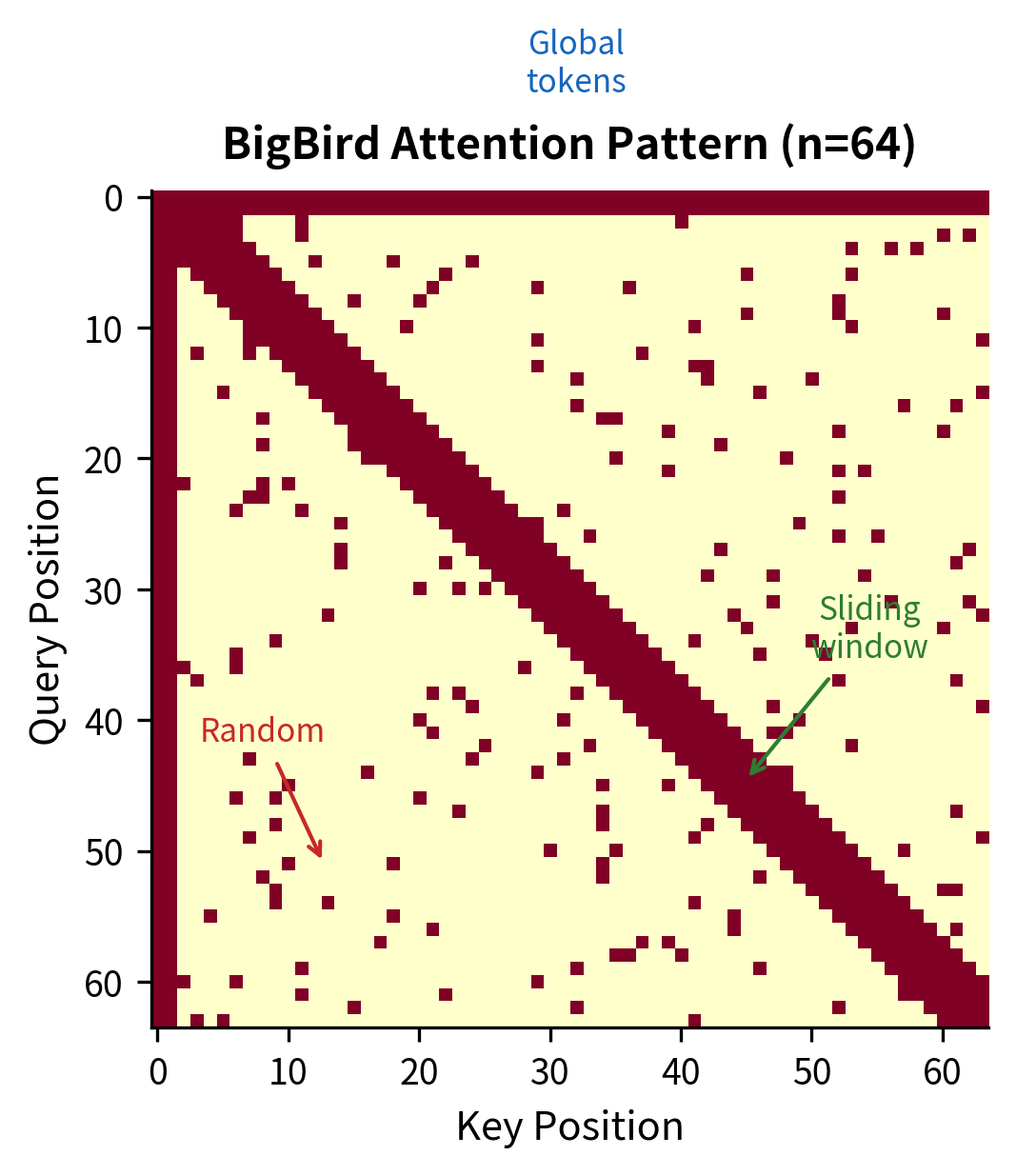
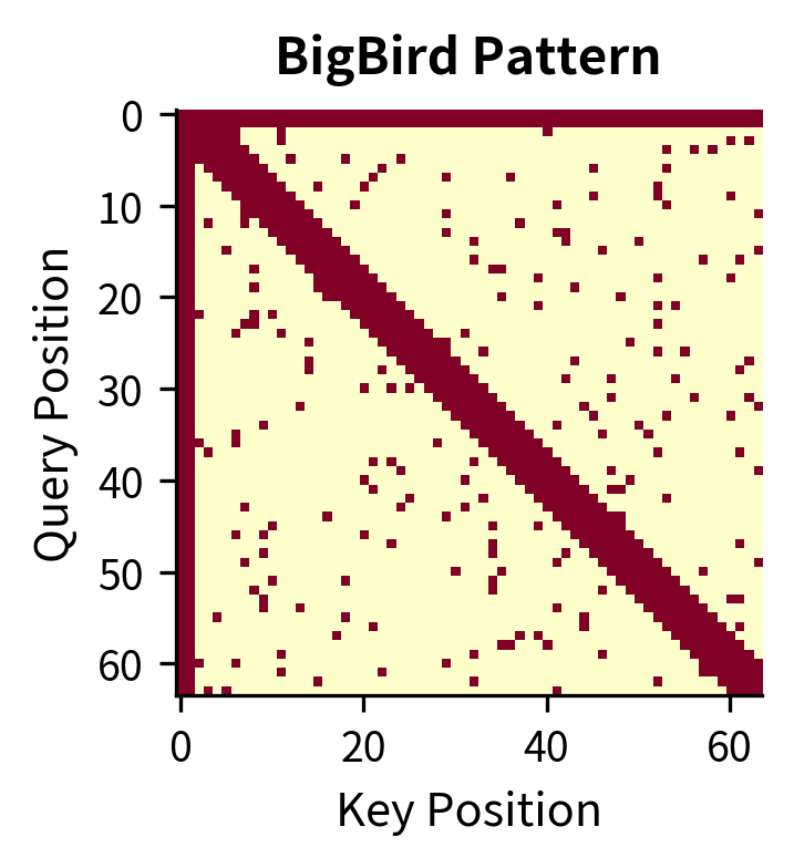
The visualization shows the three distinct components of BigBird attention. The diagonal band represents the sliding window, capturing local dependencies. The rows and columns at the edges correspond to global tokens. The scattered points outside the diagonal band are random attention connections, which we'll see are crucial for the model's theoretical properties.
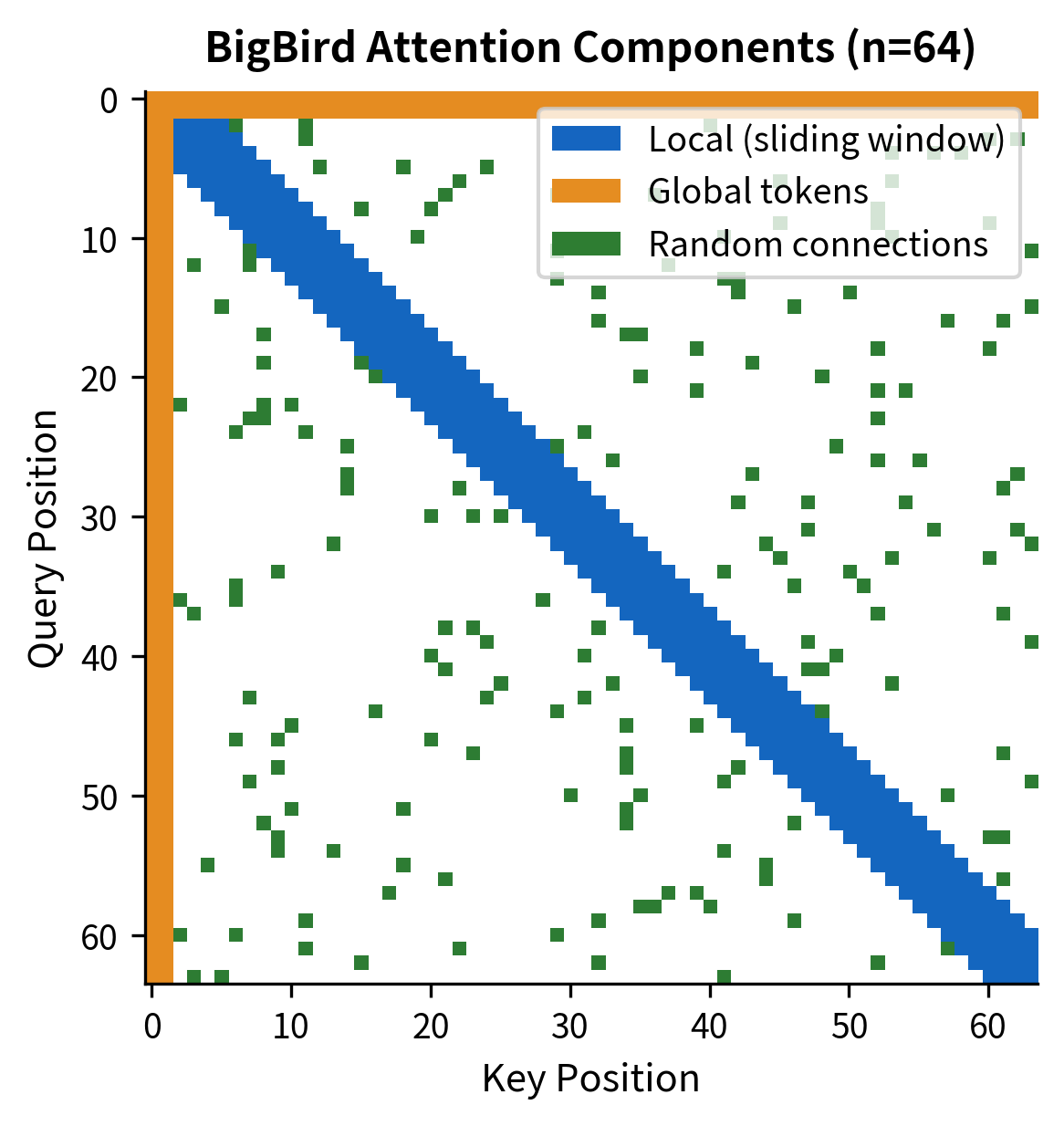
The color-coded visualization makes each component's contribution clear. The blue diagonal band captures the sliding window pattern, ensuring every token sees its immediate neighbors. The orange bars at the top and left edges represent the global tokens, which can communicate with any position in the sequence. The scattered green dots are the random connections, sparse but strategically placed to reduce the graph diameter.
Why Random Attention Works
We've claimed that random attention connections have deep theoretical significance, but why exactly? To understand this, we need to think about attention patterns as graphs and consider how information propagates through them.
The Graph Theory Perspective
The key insight is to view attention as a communication network. Each token is a node, and an attention connection is a directed edge along which information can flow. When token attends to token , information from 's representation contributes to 's output. Over multiple layers, information propagates along paths in this graph.
Formally, consider the attention pattern as a directed graph where each token is a node, and there's an edge from token to token if attends to :
The diameter of this graph is the maximum shortest path length between any two nodes:
where is the shortest path length from node to node .
With only local sliding window attention, the diameter is . To understand why, consider passing information from token 1 to token . Each attention layer can propagate information by at most positions in either direction. Therefore, you need at least layers (or attention hops) to bridge the gap. This limits how deep information can flow in a fixed number of layers.
Adding random connections reduces the diameter to with high probability. This is a well-known result from random graph theory: even a small number of random edges create shortcuts that connect distant regions of the graph. These shortcuts mean that any two nodes can reach each other in logarithmic rather than linear steps.
The measured diameters closely match theoretical predictions. With local-only attention, information must hop through roughly 42 positions to traverse the sequence, but BigBird's random connections create shortcuts that reduce this to just a handful of hops. This dramatic reduction means information can propagate between any two tokens in just a few attention layers. This is essential for tasks requiring long-range reasoning, such as understanding that a pronoun at position 500 refers to an entity introduced at position 50.
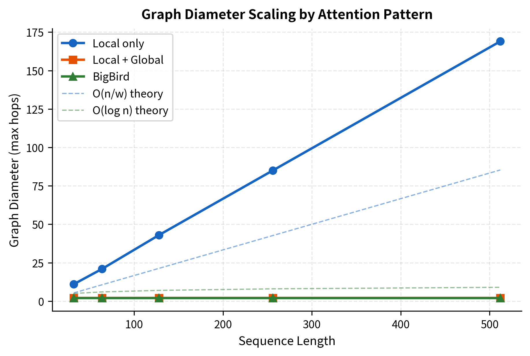
The visualization confirms the theoretical predictions. Local-only attention diameter grows linearly, closely following the curve. BigBird's diameter stays nearly flat, following the curve. This logarithmic scaling is the key to BigBird's ability to handle long sequences: even for 16,384-token documents, information only needs about 14 hops to travel end-to-end.
Theoretical Guarantees
The practical benefits of reduced graph diameter translate into formal theoretical guarantees. The BigBird paper provides three key proofs about the expressiveness of their sparse attention pattern:
1. Turing Completeness. BigBird sparse attention can simulate any Turing machine. This proves that the sparse pattern is computationally universal. Any computation that can be performed by a standard transformer (which is Turing complete) can also be performed by a BigBird transformer. The random connections are essential for this proof because they ensure the attention graph is well-connected enough to route information arbitrarily.
2. Universal Approximation. Any sequence-to-sequence function computed by a full attention transformer can be approximated by a BigBird transformer with only random connections per position. You don't need many random connections. A constant number per token, regardless of sequence length, is sufficient. The proof relies on showing that the BigBird pattern can simulate a star graph (where one central node connects to all others), which in turn can simulate full attention.
3. Star Graph Simulation. The combination of global and random attention can simulate the star graph topology, which is sufficient for full attention approximation. Intuitively, any full attention computation can be decomposed into: (a) aggregating information at a central hub, (b) processing it, and (c) distributing results back. The global tokens provide the hub, and random connections ensure the hub can reach any position efficiently.
These results provide confidence that BigBird's sparse pattern doesn't fundamentally limit what the model can learn. The efficiency gains come from reducing constant factors and exploiting the structure of natural data, not from sacrificing expressive power. When BigBird performs worse than full attention on some task, it's because the learned attention patterns happened to need dense connections, not because the architecture is inherently less capable.
Implementing BigBird Attention
Now that we understand the three components and their theoretical justification, let's implement a complete BigBird attention layer. This implementation will help solidify the concepts and show how the sparse pattern translates into actual computation.
The implementation follows the standard attention pipeline with one key modification: we apply a sparse mask before the softmax to zero out attention scores for non-attended positions. This mask encodes our three-component pattern: local windows, global tokens, and random connections.
The output shape matches the input, confirming that BigBird attention preserves sequence dimensions. Each token attends to approximately 26 positions on average, which aligns with our theoretical expectation of . The 89.7% sparsity means we're computing less than 11% of the attention scores that full attention would require.
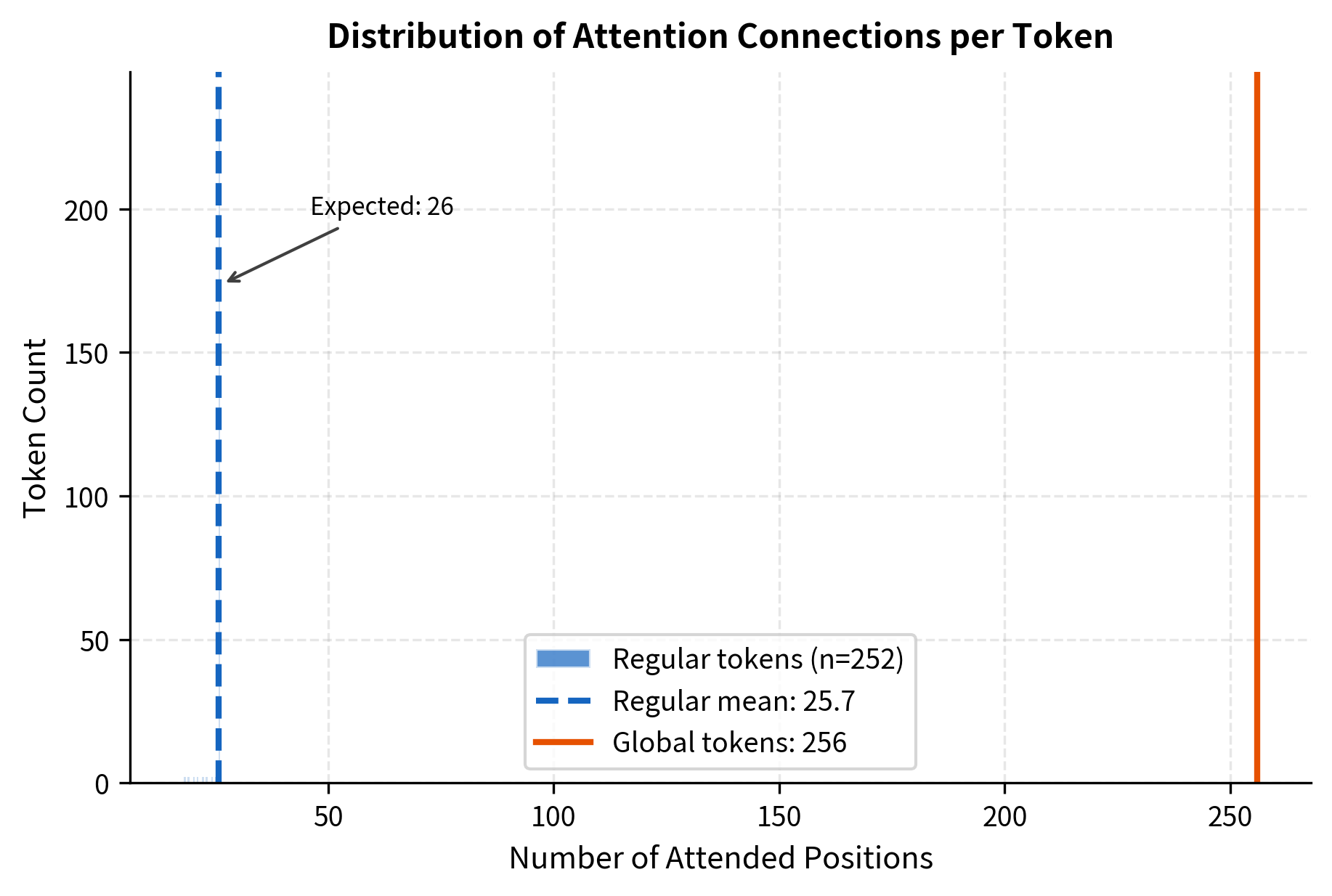
The histogram reveals the bimodal nature of BigBird's connection pattern. Regular tokens cluster tightly around the expected value of , reflecting the consistent sparse pattern. The few global tokens (positions 0-3) attend to all positions, appearing at the far right. This structure ensures that most of the computation is bounded while still maintaining global connectivity through the hub tokens.
The implementation shows that each token attends to roughly other tokens, independent of sequence length. More precisely, for a token at position (excluding the first global tokens), the number of attended positions is:
where some positions may overlap (e.g., if a random connection happens to fall within the local window or on a global token). The global tokens themselves attend to all positions, but since there are only of them, this adds total connections. This bounded fan-out per token is the source of BigBird's linear complexity.
Comparing BigBird and Longformer
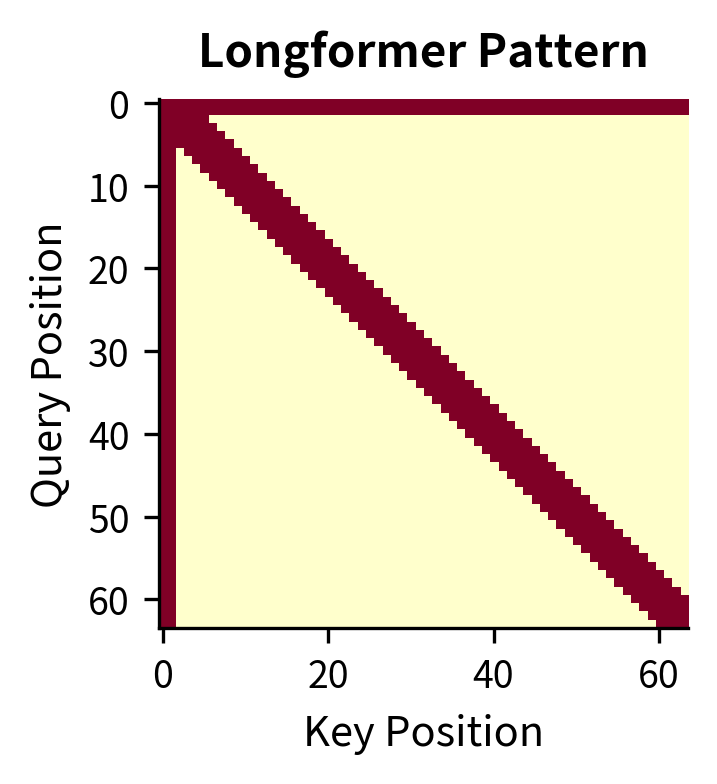
BigBird and Longformer are both sparse attention models designed for long documents, but they differ in one crucial aspect: random attention. Let's compare their attention patterns and understand the trade-offs.
The random attention component adds only about 30% more connections compared to Longformer. This modest overhead is the price for BigBird's stronger theoretical guarantees. In practice, both patterns achieve similar downstream performance on most tasks, but BigBird's random connections ensure the model can theoretically approximate any full-attention computation.
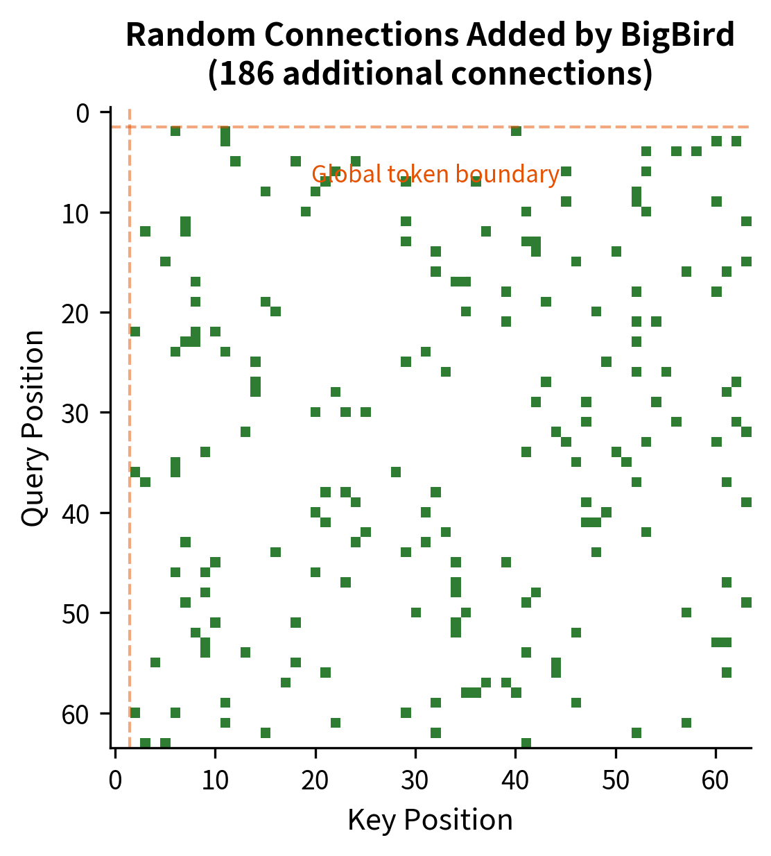
The visualization highlights exactly where BigBird differs from Longformer. Each green point represents a random attention connection, the shortcuts that reduce graph diameter from linear to logarithmic. Note how these connections are distributed across the entire sequence, ensuring that no region is isolated.
The visual difference is subtle, as the random connections are sparse. However, the theoretical implications are significant:
| Property | Longformer | BigBird |
|---|---|---|
| Local attention | Yes | Yes |
| Global tokens | Yes | Yes |
| Random attention | No | Yes |
| Graph diameter | ||
| Turing complete | Not proven | Proven |
| Universal approximator | Not proven | Proven |
The graph diameter difference is particularly important: means that for a sequence of 4,096 tokens with window size 64, Longformer needs roughly 64 attention hops to propagate information end-to-end. BigBird with random connections needs only about hops.
In practice, both models perform well on long-document tasks, and the choice often depends on the specific application. Longformer's deterministic pattern is easier to optimize with custom CUDA kernels, while BigBird's random connections provide stronger theoretical guarantees.
Complexity Analysis
Let's analyze the computational and memory complexity of BigBird attention compared to standard full attention:
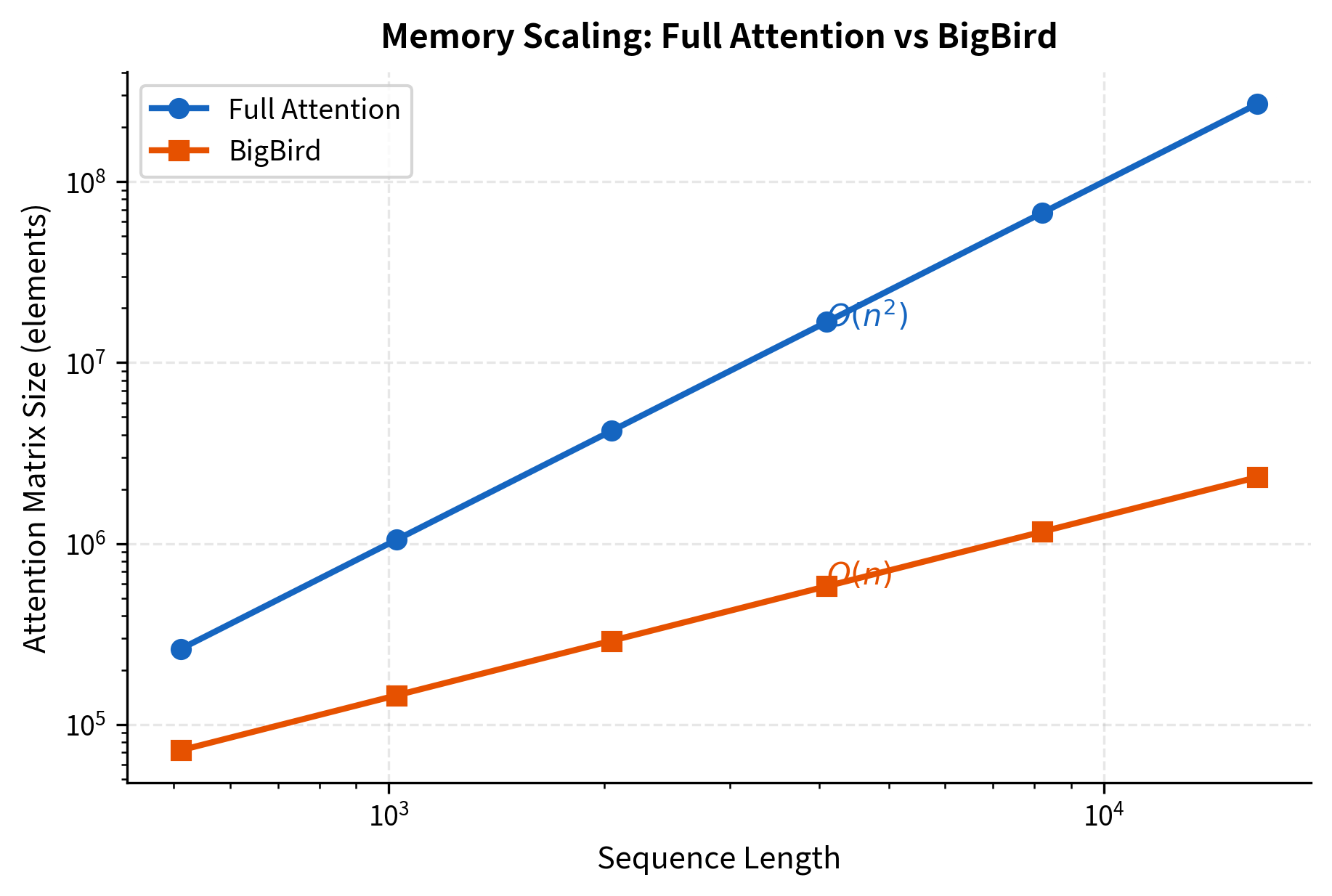
The log-scale plot clearly shows the difference between quadratic and linear scaling. For full attention, the number of attention scores is:
For BigBird, the approximate number is:
where:
- : sequence length
- : number of global tokens (which each attend to all positions)
- : one-sided window size
- : number of random connections per non-global token
At 4,096 tokens, full attention requires 16 million attention scores. BigBird, with its sparse pattern, needs only about 600,000, a roughly 25x reduction. At 16,384 tokens, the gap widens to nearly 100x.
BigBird Applications
BigBird's ability to handle long sequences opens up applications that were previously impractical with standard transformers.
Document Understanding
Legal contracts, scientific papers, and financial reports often span thousands of tokens. BigBird can process entire documents in a single forward pass, enabling:
- Document classification without truncation
- Long-form question answering where the answer might be far from relevant context
- Document summarization that captures themes from throughout the text
Genomics
DNA sequences can be millions of base pairs long, with meaningful patterns spanning thousands of positions. BigBird's linear complexity makes it feasible to model these sequences, enabling:
- Variant effect prediction
- Gene expression modeling
- Protein function prediction from genomic context
Long-Context Retrieval
Information retrieval tasks often benefit from considering entire documents rather than short passages. BigBird enables:
- Dense retrieval with full document encoding
- Cross-document reasoning
- Citation analysis and document linking
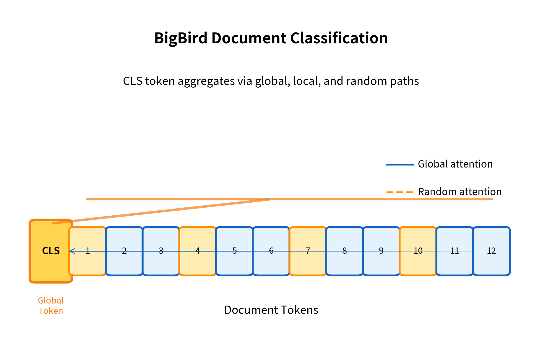
A Worked Example: Long Document Classification
Let's trace through how BigBird processes a long document classification task:
The table shows that as document length increases, the sparsity remains roughly constant (determined by window size, global tokens, and random connections), while the memory savings grow dramatically. An 8,192-token document that would require 256 MB for full attention needs only about 5 MB with BigBird's sparse pattern.
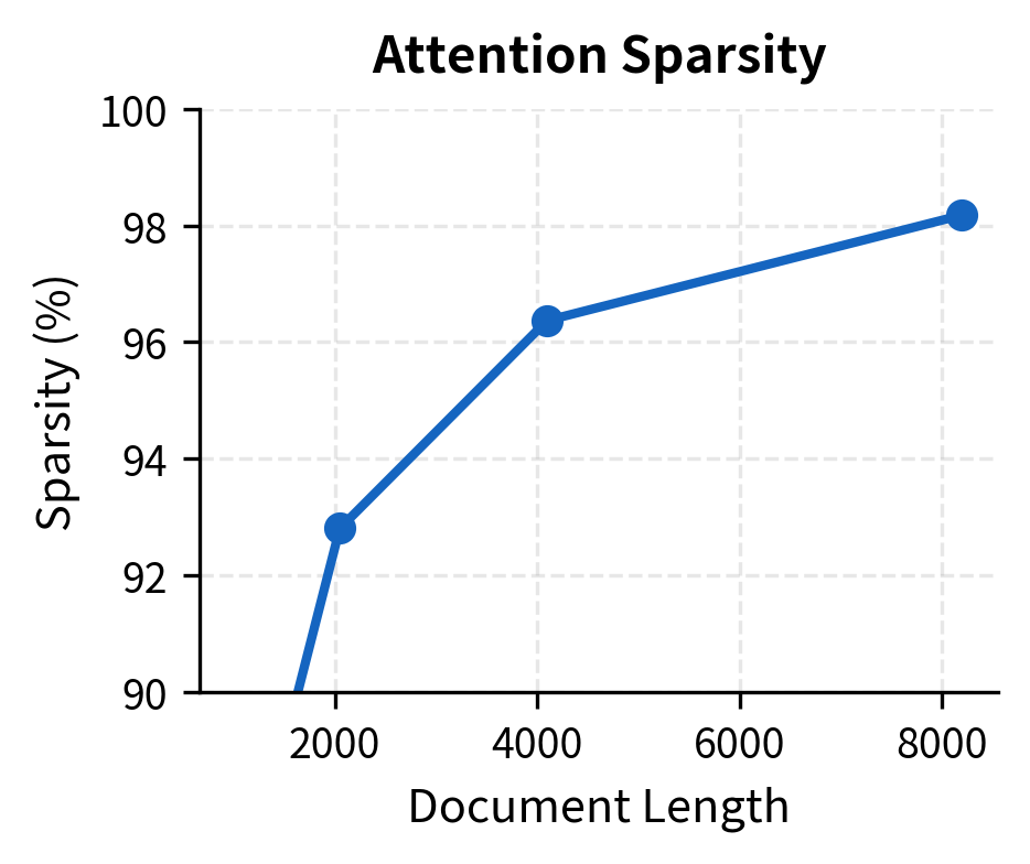
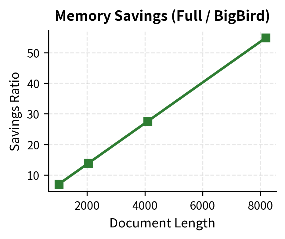
The left panel shows that sparsity increases steadily as documents get longer, reaching over 98% for 8K-token documents. The right panel shows the corresponding memory savings: because full attention grows quadratically while BigBird grows linearly, the savings ratio itself grows linearly with sequence length. This means longer documents benefit even more from BigBird's sparse pattern.
Limitations and Impact
BigBird represents a significant advance in efficient attention mechanisms, but it comes with trade-offs that affect its practical deployment.
The most significant limitation is implementation complexity. While the attention pattern achieves linear theoretical complexity, realizing this in practice requires careful engineering. The random attention component prevents the use of simple blocked matrix operations, and naive implementations may not achieve the expected speedups. Libraries like HuggingFace Transformers provide optimized BigBird implementations, but custom CUDA kernels are needed for maximum efficiency.
Another consideration is the fixed attention pattern. Once the window size, number of global tokens, and number of random connections are set, the pattern doesn't adapt to input content. Some documents might benefit from more local attention (technical text with nearby dependencies) while others need more global attention (narratives with long-range references). The fixed pattern is a one-size-fits-all solution that may not be optimal for every input.
The random connections also introduce non-determinism during training if new random patterns are sampled for each forward pass. Most implementations fix the random seed for reproducibility, but this means the model learns to rely on a specific random pattern rather than arbitrary connections. Whether this matters in practice depends on the downstream task.
Despite these limitations, BigBird has had substantial impact on long-document NLP. It demonstrated that sparse attention can match full attention on most benchmarks while scaling to much longer sequences. The theoretical results showing Turing completeness and universal approximation provided formal justification for the sparse attention paradigm. Google used BigBird for their Pegasus-X model, and the architecture influenced subsequent work on efficient transformers including LongT5 and LED (Long-document Encoder-Decoder).
The key insight from BigBird, that random attention connections provide theoretical guarantees while adding minimal computational overhead, has influenced the design of many subsequent efficient attention mechanisms.
Summary
BigBird extends the sparse attention paradigm by adding random attention connections to the local-window-plus-global-tokens pattern pioneered by Longformer. This addition is not arbitrary: random connections reduce the graph diameter from to , where is the sequence length and is the window size. This logarithmic diameter enables efficient information propagation across the entire sequence in just a few attention layers.
Key takeaways from this chapter:
-
Three-component attention: BigBird combines sliding window attention for local context, global tokens for long-range hubs, and random attention for shortcuts between distant positions. Each component serves a distinct purpose in maintaining model expressiveness.
-
Theoretical guarantees: The BigBird paper proved that their sparse pattern is Turing complete and can approximate any sequence-to-sequence function computable by full attention. The random connections are crucial for these proofs.
-
Linear complexity: BigBird achieves time and memory complexity by fixing the number of attended positions per token to a constant independent of sequence length.
-
Graph diameter reduction: Random attention connections act as shortcuts in the attention graph, reducing the diameter from linear to logarithmic and enabling information to flow between any two positions in just a few layers.
-
Practical trade-offs: While theoretically elegant, BigBird requires careful implementation to realize its efficiency gains. The fixed attention pattern may not be optimal for all inputs.
-
Applications: BigBird enables processing of long documents (legal, scientific, financial), genomic sequences, and other domains where context windows of 4K-16K tokens are needed.
The next chapter explores linear attention mechanisms, which take a fundamentally different approach to efficiency by reformulating the attention computation to avoid materializing the attention matrix entirely.
Key Parameters
When configuring BigBird attention, several parameters control the trade-off between efficiency and model expressiveness:
-
window_size: The one-sided sliding window size, determining how many neighbors each token attends to on each side. Larger windows capture more local context but increase computation. Typical values range from 64 to 256. For most NLP tasks, 128 provides a good balance.
-
num_global: The number of global tokens that attend to and are attended by all other tokens. These serve as information hubs for long-range communication. Common choices are 2-8 tokens. Using the
[CLS]token plus sentence-start markers is a practical approach. -
num_random: The number of random attention connections per non-global token. This parameter is crucial for BigBird's theoretical guarantees. Values of 3-5 are typically sufficient to achieve logarithmic graph diameter. Increasing beyond 5 provides diminishing returns.
-
block_size: In optimized implementations, attention is computed in blocks for efficiency. Common values are 64 or 128. This should divide evenly into your sequence length.
-
attention_type: BigBird supports two modes:
"original_full"computes full attention for short sequences (faster when ), while"block_sparse"uses the sparse pattern. Most libraries automatically select based on sequence length.
The interplay between these parameters determines the effective receptive field and computational cost. For a sequence of length with window size , global tokens, and random connections, the total attention operations scale as , which remains linear as long as these hyperparameters are constants.
Quiz
Ready to test your understanding? Take this quick quiz to reinforce what you've learned about BigBird sparse attention.

Comments