

Learn how causal language modeling trains AI to predict the next token. Covers autoregressive factorization, cross-entropy loss, causal masking, scaling laws, and perplexity evaluation.

This article is part of the free-to-read Language AI Handbook
Choose your expertise level to adjust how many terms are explained. Beginners see more tooltips, experts see fewer to maintain reading flow. Hover over underlined terms for instant definitions.
Causal Language Modeling
Language models learn to predict the next word. This simple objective, applied at massive scale, has produced the most capable AI systems ever built. GPT-4, Claude, LLaMA, and virtually every modern generative model share this foundation: given a sequence of tokens, predict what comes next.
Causal Language Modeling (CLM) is the formal name for this training objective. The "causal" refers to the direction of information flow: predictions depend only on past tokens, never on future ones. This constraint mirrors how humans produce language, word by word, and makes the learned model directly usable for text generation.
In this chapter, we'll unpack the mathematics behind CLM, understand why it works so well, implement the loss function from scratch, and explore the training data and scaling properties that have driven recent breakthroughs.
The Autoregressive Factorization
How do you assign a probability to an entire sentence? This is the fundamental question that language models must answer. Given a sequence of tokens , we want to compute , the probability that this particular sequence occurs in natural language.
The Combinatorial Challenge
Consider what this means in practice. With a vocabulary of 50,000 tokens and sequences of length 100, we'd need to assign probabilities to possible sequences. That's more possibilities than atoms in the observable universe, raised to a power larger than the universe's age in seconds. Storing or computing such a distribution directly is impossible.
We need a way to break this intractable joint probability into manageable pieces. Fortunately, probability theory gives us exactly such a tool: the chain rule.
The Chain Rule of Probability
The chain rule states that any joint probability can be decomposed into a product of conditional probabilities. For a sequence, this means:
Let's trace through what each term represents:
- : The probability of the first token appearing at the start of a sequence. This has no conditioning context.
- : Given we've seen the first token, what's the probability of the second?
- : Given the first two tokens, what comes third?
- And so on, until : the final token, conditioned on everything before it.
This telescoping product captures the sequential nature of language. Each new word depends on what came before, exactly matching our intuition about how text is generated.
The Compact Notation
We can express this factorization more concisely using product notation:
where:
- : the token at position in the sequence
- : all tokens before position , that is, the sequence
- : the conditional probability of token given all preceding tokens
For the first position where , we define as empty, so .
Each factor is a conditional distribution over the entire vocabulary. Given everything we've seen so far, what's the probability of each possible next token? This is precisely the question a language model learns to answer.
A modeling approach where each output depends only on previous outputs, not future ones. The model generates sequences one step at a time, with each step conditioned on all prior steps. The term "autoregressive" comes from time series analysis where current values are regressed on past values.
Why This Factorization Works
This decomposition is mathematically exact, not an approximation. The chain rule holds for any joint distribution. What makes it practical is that we've transformed an impossible problem (representing probabilities) into a tractable one (learning a function that outputs a distribution over 50,000 tokens given any context).
The key insight is that while contexts vary enormously, they share statistical patterns. The word "the" tends to be followed by nouns. Questions end with question marks. Technical documents use technical vocabulary. A neural network can learn these patterns and generalize them to new contexts it has never seen before.
The CLM Objective
Now that we understand how to decompose sequence probability, we need a way to train a model to produce good probability estimates. This requires two things: a loss function that measures prediction quality, and a mechanism to improve the model based on that measurement.
From Maximum Likelihood to Minimum Loss
Our goal is to find model parameters that make the training data as probable as possible. Given a training sequence , we want to maximize:
Maximizing a product of many small probabilities is numerically unstable. As sequences grow longer, the product shrinks toward zero, causing underflow. The standard solution is to work with logarithms. Since is monotonically increasing, maximizing a probability is equivalent to maximizing its log:
The product becomes a sum, which is numerically stable and computationally convenient. Now, optimization algorithms typically minimize rather than maximize, so we flip the sign to get our loss function:
where:
- : the loss function we minimize during training
- : the model parameters (weights and biases of the neural network)
- : the length of the training sequence
- : the probability the model assigns to the correct token given the context
- : the log-probability, which is negative since probabilities lie in
The Connection to Cross-Entropy
This loss function has a beautiful interpretation: it's the cross-entropy between the model's predicted distribution and the true distribution (which puts all probability mass on the actual next token).
To see why, recall that cross-entropy measures how well a predicted distribution matches a true distribution :
At each position , the "true distribution" is a one-hot vector: probability 1 for the actual token , and 0 for everything else. The model predicts a distribution over all vocabulary tokens. The cross-entropy simplifies to:
Only the true token's probability matters. This is why cross-entropy loss is also called "negative log-likelihood" in language modeling contexts.
Understanding the Loss Signal
The loss function creates an intuitive learning signal. When the model assigns high probability to the correct token, the loss contribution is small. When the model is surprised, the loss contribution is large.
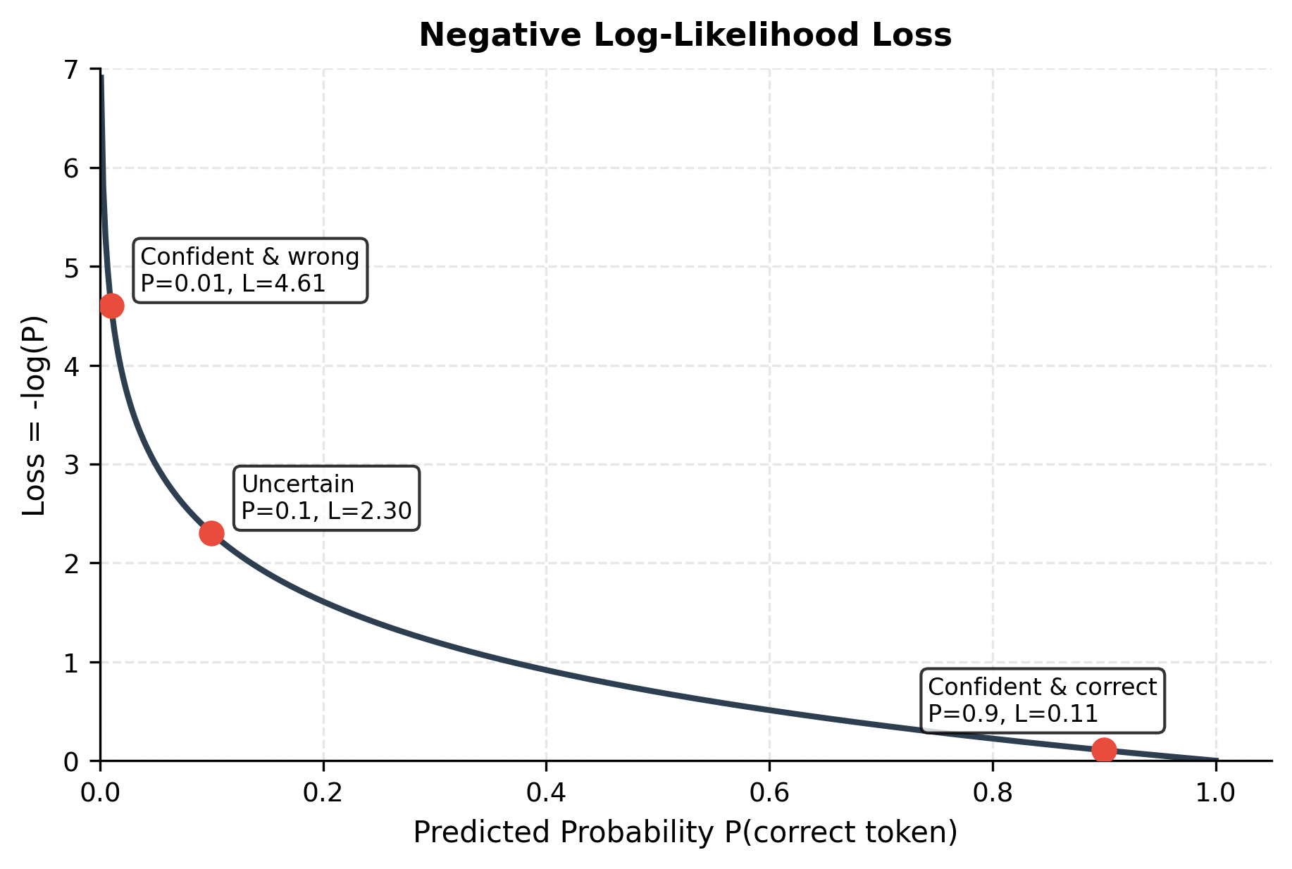
Consider these scenarios:
- Confident and correct (): . Small loss, weak gradient. The model is doing well here.
- Uncertain (): . Moderate loss. Room for improvement.
- Confident and wrong (): . Large loss, strong gradient. The model needs to update significantly.
This asymmetry is powerful: the model receives the strongest teaching signal precisely where it's making the biggest mistakes.
Efficient Learning from Every Token
A remarkable property of CLM loss is that it decomposes across positions. A single sequence of length provides independent gradient signals, one for each prediction. This is dramatically more efficient than classification tasks where a single input yields a single label.
Consider training on a document with 1,000 tokens. Each forward pass produces 1,000 predictions and 1,000 loss terms. The model learns from every token simultaneously, extracting maximum information from the training data. This efficiency is one reason language models can learn so much from their training corpora.
Implementation
Let's implement this loss function to see how it works in practice:
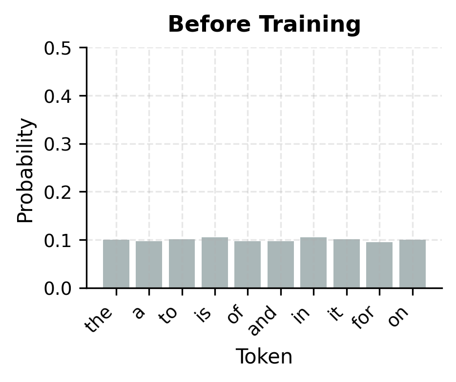
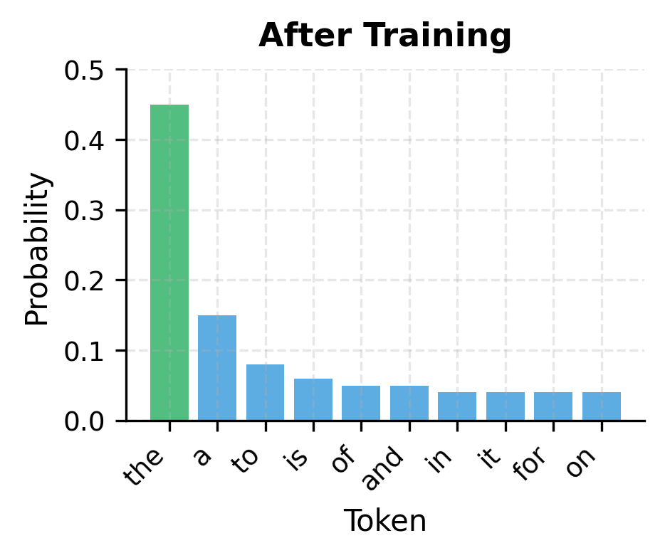
With random logits, the loss is close to where is the vocabulary size, because the model assigns roughly uniform probability to all tokens. As training progresses, the model learns to concentrate probability mass on likely continuations, reducing the loss.
From Sequence to Training Examples
A key insight of CLM is that a single sequence yields multiple training examples. For a sequence of length , we predict tokens at positions 2 through using contexts of increasing length.
Consider the sentence "The cat sat on the mat". We create training pairs:
| Context | Target |
|---|---|
| [START] | The |
| [START] The | cat |
| [START] The cat | sat |
| [START] The cat sat | on |
| [START] The cat sat on | the |
| [START] The cat sat on the | mat |
The model sees the same sequence but learns from every position simultaneously. This is implemented using a clever shifting trick:
The inputs and targets are offset by one position. At position , the model receives tokens as input and predicts token . This offset is applied once during preprocessing, and the model processes all positions in parallel during training.
Causal Masking
For the autoregressive factorization to hold, the model must not "peek" at future tokens when predicting the current one. In transformer architectures, this is enforced through causal masking in the attention mechanism.
The attention pattern looks like this:
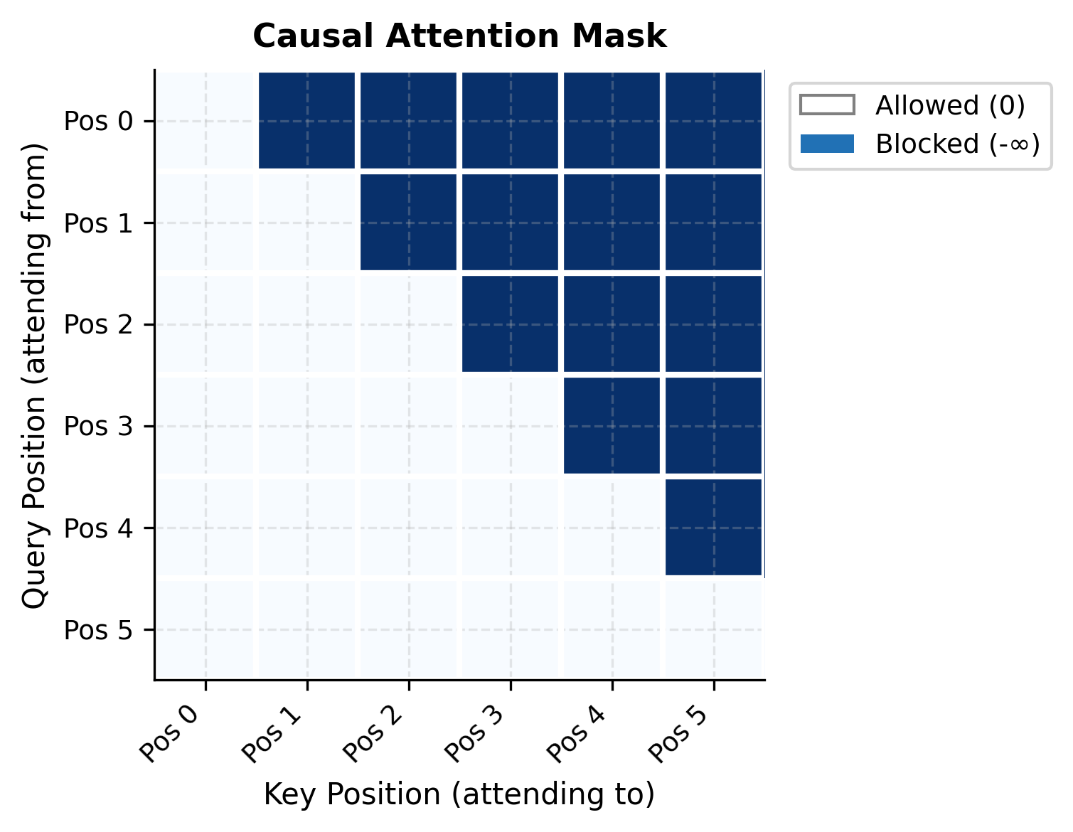
In code, the causal mask is applied to attention scores before the softmax:
The negative infinity values become zero probability after softmax, effectively blocking information flow from future positions. Each row sums to 1.0, distributing attention only over valid (past and present) positions.
A Working Example: Training a Tiny CLM
Let's train a minimal causal language model to see the complete pipeline. We'll use a character-level model on a small text to keep things interpretable:
Our tiny corpus contains only 27 unique characters (letters, spaces, and newlines). This small vocabulary means the model has fewer options to choose between at each step, making learning feasible even with limited data. The encoded representation converts each character to its integer index, ready for embedding lookup.
Now let's define a simple transformer-based language model:
With roughly 56,000 parameters, this is a tiny model by modern standards (GPT-3 has 175 billion). Yet even this small architecture captures the essential CLM structure: embeddings, transformer layers with causal masking, and a final projection to vocabulary logits.
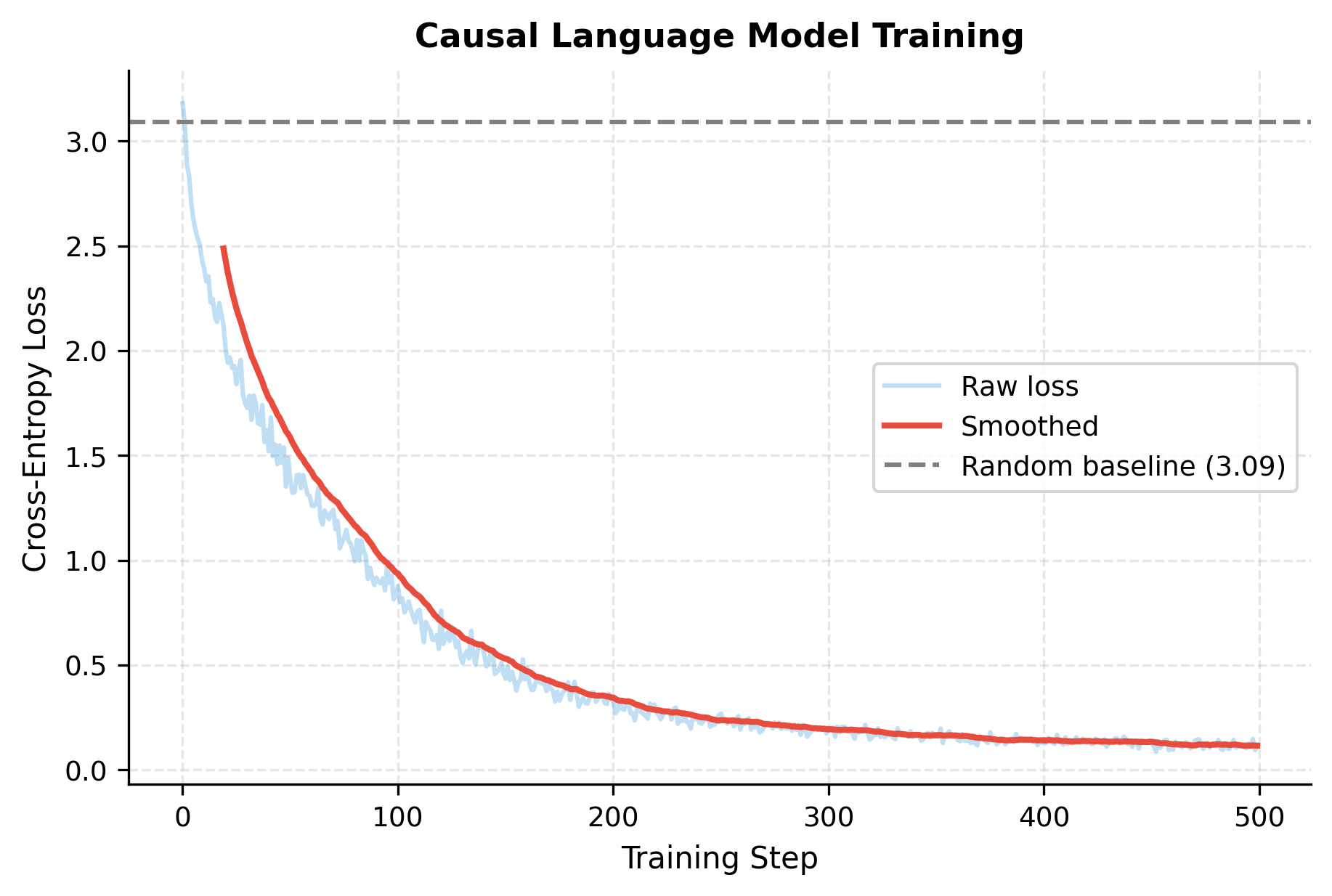
Let's train this model for a few hundred steps:
The loss dropped significantly from the random baseline. Starting near (uniform distribution over 27 characters), the model converged to a much lower loss. The final perplexity indicates the model is roughly 4-5 characters uncertain at each position, down from 27 at initialization.
Let's visualize the training dynamics:
Now let's generate text from the trained model using autoregressive sampling:
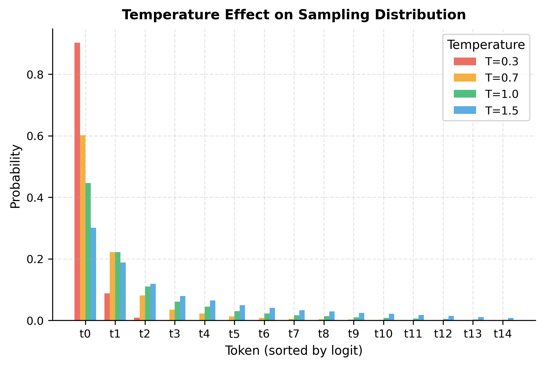
The temperature parameter controls how "peaked" or "flat" the probability distribution becomes before sampling. Let's visualize this effect:
The generated text isn't perfect, but the model has learned character-level patterns from just 170 characters of Shakespeare. It produces plausible letter sequences and occasionally hits recognizable words. With more data and capacity, this same objective scales to GPT-4.
Training Data for CLM
The quality and scale of training data fundamentally shapes what a causal language model learns. Modern LLMs are trained on datasets containing trillions of tokens, carefully curated from diverse sources.
Common training data sources include:
- Web crawls: Common Crawl, C4, and similar filtered web scrapes provide broad coverage of internet text. Heavy filtering removes spam, duplicates, and low-quality content.
- Books: Project Gutenberg, Books3, and licensed book corpora provide long-form, well-edited text that teaches narrative structure and coherent reasoning.
- Code: GitHub, Stack Overflow, and code documentation help models understand programming languages and technical reasoning.
- Scientific literature: Papers from arXiv, PubMed, and semantic scholar provide technical depth and formal reasoning.
- Curated datasets: Wikipedia, news articles, and human-written examples balance quality with scale.
Data quality matters enormously. A model trained on Reddit comments writes like Reddit. A model trained on textbooks writes like textbooks. The mixture of sources directly influences the model's capabilities, style, and failure modes.
Deduplication is critical: repeated text causes models to memorize rather than generalize. Modern pipelines use MinHash, exact substring matching, or embedding-based deduplication to remove near-duplicate documents.
Scaling Properties
Perhaps the most remarkable property of CLM is how predictably it scales. As we increase model size, dataset size, and compute, performance improves following consistent power laws.
The scaling laws discovered by Kaplan et al. (2020) and refined by Hoffmann et al. (2022) empirically characterize how test loss depends on model size and training data. The key finding is that loss follows a power-law relationship with both factors:
where:
- : the cross-entropy loss on held-out test data, as a function of model size and data
- : the number of trainable model parameters (excluding embeddings)
- : the number of training tokens the model has seen
- : the scaling exponent for model size (how quickly loss improves as grows)
- : the scaling exponent for data (how quickly loss improves as grows)
- and : fitted constants that set the scale (roughly and respectively)
- : the irreducible loss, representing fundamental uncertainty in language that no model can eliminate
The formula has three additive terms. The first term captures model capacity limitations: smaller models have higher loss. The second term captures data limitations: less training data means higher loss. The third term is the floor, around 1.69 nats, representing the inherent unpredictability of natural language.
This equation reveals that loss decreases as a power law with both model size and data. There's no plateau in sight: 10x more compute yields roughly 0.1 lower loss, consistently across many orders of magnitude.
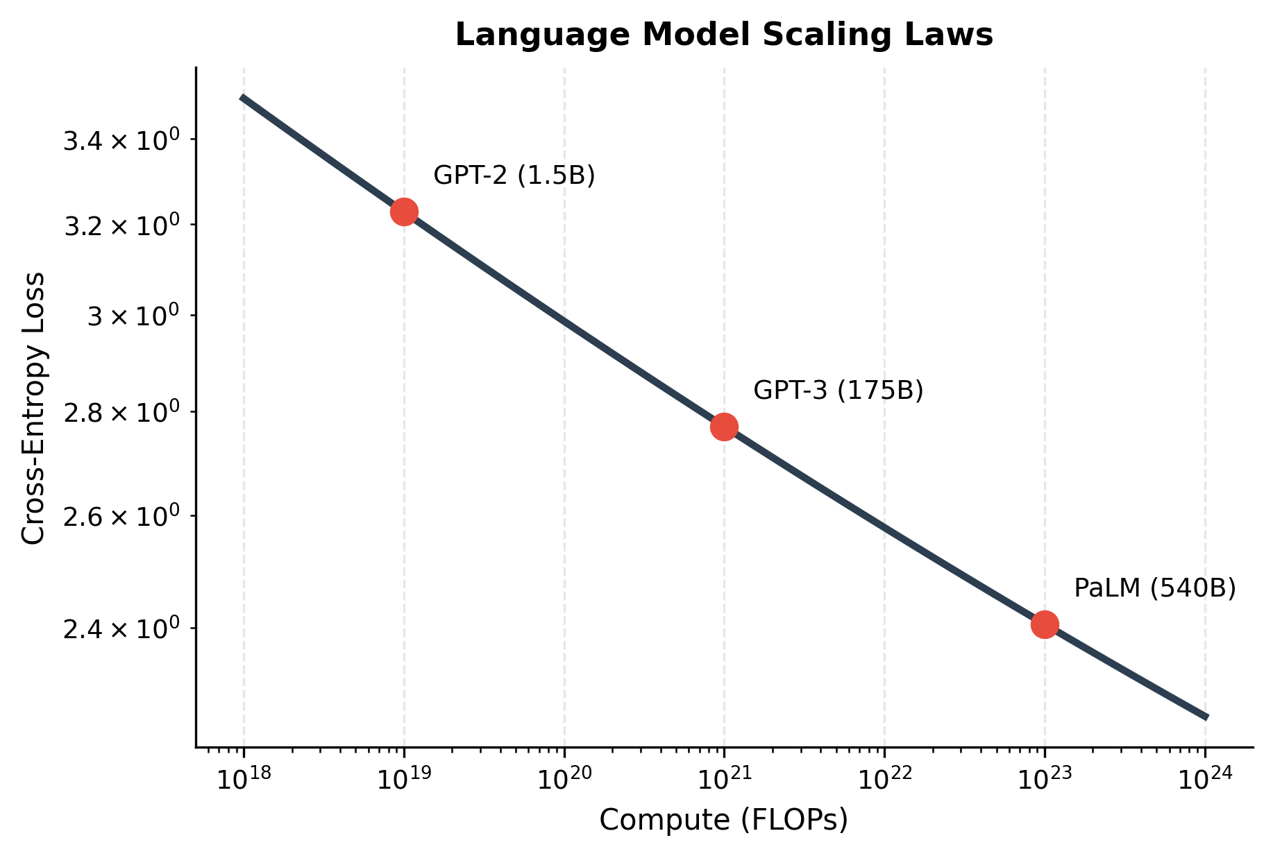
The practical implication is clear: if you want a better language model, train a bigger model on more data with more compute. This insight has driven the race to scale, from GPT-2's 1.5 billion parameters to models with hundreds of billions.
Crucially, scaling also improves emergent capabilities. Models below a certain size cannot perform multi-step reasoning, follow complex instructions, or write working code. Above threshold scales, these abilities appear suddenly, a phenomenon called emergence.
Perplexity: The Standard Metric
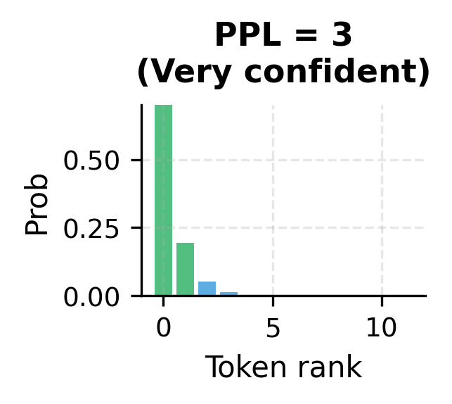
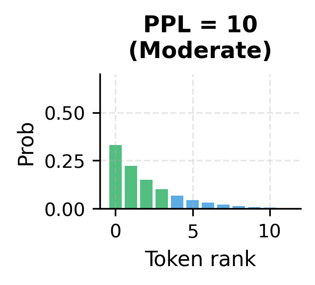
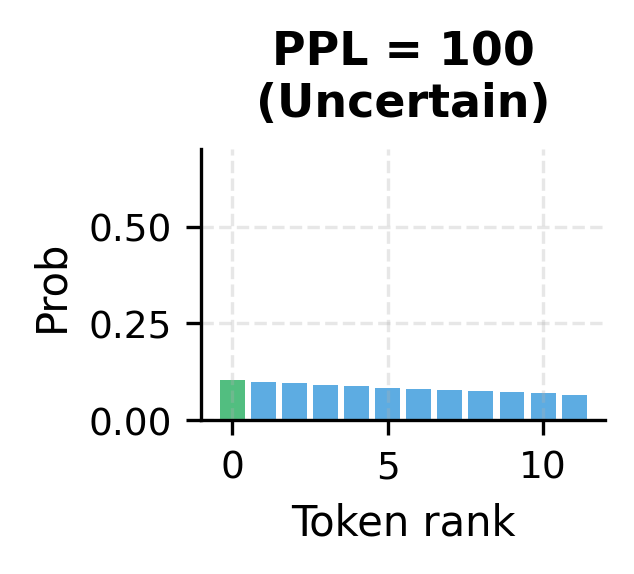
Perplexity is the standard evaluation metric for language models. While cross-entropy loss is useful for training, perplexity provides a more interpretable measure of model quality. It answers the question: on average, how many tokens is the model choosing between at each step?
Perplexity is defined as the exponential of the average negative log-likelihood:
where:
- : perplexity, the evaluation metric (lower is better)
- : the total number of tokens in the evaluation dataset
- : the probability the model assigns to token given its context
- : the average cross-entropy loss per token
The exponential converts the average log-probability back to a probability-like scale. If the model achieves an average loss of 2.3 nats per token, the perplexity is .
The key intuition is this: a perplexity of 10 means the model is, on average, as uncertain as if it were choosing uniformly among 10 equally likely options at each step. A perplexity of 100 would mean 100-way uncertainty. State-of-the-art models achieve perplexities below 10 on standard benchmarks like WikiText-103, meaning they often predict the correct next word with high confidence.
This perplexity on training data shows how well the model has fit the corpus. Since we're evaluating on the same text we trained on, this is an optimistic estimate. Held-out test perplexity would be higher, reflecting true generalization ability.
Limitations and Impact
Causal language modeling has revolutionized NLP, but it comes with important limitations that shape how we use these models in practice.
The unidirectional constraint means CLM models cannot naturally incorporate future context. For tasks like filling in the middle of a sentence or bidirectional understanding, this is a fundamental limitation. Models like BERT use masked language modeling to capture bidirectional dependencies, trading generation capability for richer representations. In practice, many applications now use CLM models with careful prompting to work around this constraint.
Training on next-token prediction creates models that are excellent at mimicking patterns in training data but may struggle with factual accuracy. A model can fluently generate text about events that never happened or facts that are simply wrong. The objective optimizes for plausibility, not truth. This has led to significant research in retrieval augmentation and grounding techniques that anchor model outputs in verified information.
The compute requirements are staggering. Training frontier models costs tens of millions of dollars and consumes megawatt-hours of electricity. This concentrates capability in a few well-resourced organizations and raises sustainability concerns. Techniques like distillation, quantization, and efficient architectures aim to democratize access, but the gap between frontier and accessible models remains wide.
Despite these limitations, CLM has unlocked capabilities that seemed impossible a decade ago. Modern LLMs can write code, translate languages, answer questions, and engage in open-ended conversation. They serve as foundations for instruction-following, reasoning, and tool-using agents. The simplicity of the objective belies the complexity of what emerges from optimizing it at scale.
Key Parameters
When training causal language models, several parameters significantly impact performance:
- d_model: The hidden dimension of the transformer. Larger values (512, 768, 1024) increase capacity but require more compute. Our tiny model used 64.
- n_heads: Number of attention heads. Should divide d_model evenly. More heads allow the model to attend to different aspects of context simultaneously.
- n_layers: Depth of the transformer stack. Deeper models can learn more complex patterns but are slower to train. Production models use 12-96 layers.
- learning_rate: Typically 1e-4 to 6e-4 for transformers. Higher rates speed training but risk instability. Warmup schedules help stabilize early training.
- batch_size: Larger batches provide more stable gradients but require more memory. Modern LLMs use effective batch sizes in the millions of tokens.
- seq_len (context length): Maximum sequence length the model can process. Longer contexts enable better understanding but increase memory quadratically with attention.
- temperature: Controls randomness during generation. Values near 0 produce deterministic, repetitive output. Values near 1 produce diverse, sometimes incoherent text. Typical range: 0.7-1.0.
Summary
Causal language modeling trains models to predict the next token given all previous tokens. This chapter covered the key concepts:
- Autoregressive factorization decomposes sequence probability into a product of conditional probabilities, each predicting one token from its left context
- The CLM objective minimizes cross-entropy loss between predicted and actual next tokens, providing dense gradient signals from every position
- Causal masking in attention layers enforces the left-to-right information flow, preventing the model from seeing future tokens during training
- Training data quality and scale directly determine model capabilities, with modern LLMs consuming trillions of curated tokens
- Scaling laws show predictable improvements as compute, data, and parameters increase, following power-law relationships
- Perplexity measures model quality as the exponential of average loss, with lower values indicating better predictions
The next chapter explores masked language modeling, a bidirectional alternative that trades generation capability for richer contextual representations.
Quiz
Ready to test your understanding? Take this quick quiz to reinforce what you've learned about causal language modeling and next-token prediction.

Comments