RoBERTa: Robustly Optimized BERT Pretraining Approach

What if BERT was undertrained? That was the central question Facebook AI posed when they introduced RoBERTa in 2019. The original BERT achieved remarkable results, but its training recipe was established through limited experimentation. By systematically investigating each design choice, the RoBERTa team discovered that BERT's architecture was capable of much more. The secret wasn't a new architecture or a novel objective. It was simply training more carefully.

RoBERTa (Robustly Optimized BERT Pretraining Approach) matches and often exceeds BERT's performance without any architectural changes. The improvements come entirely from training decisions: removing the Next Sentence Prediction task, using dynamic masking, training with larger batches, training longer, and using more data. These changes seem incremental, but together they produce a model that outperforms BERT on virtually every benchmark.

In this chapter, we'll dissect each component of the RoBERTa recipe, understand why these changes matter, and implement the key differences between BERT and RoBERTa training.

BERT established the pretrain-then-fine-tune paradigm that dominates modern NLP. But its training setup was constrained by available compute and the need to explore many design choices quickly. The original paper trained BERT-base for about 1 million steps with a batch size of 256, processing roughly 3.3 billion tokens.

The RoBERTa team asked: what if we just trained longer, with more data, and removed potentially harmful design choices? Their experiments revealed that BERT's reported performance was nowhere near the ceiling for its architecture.

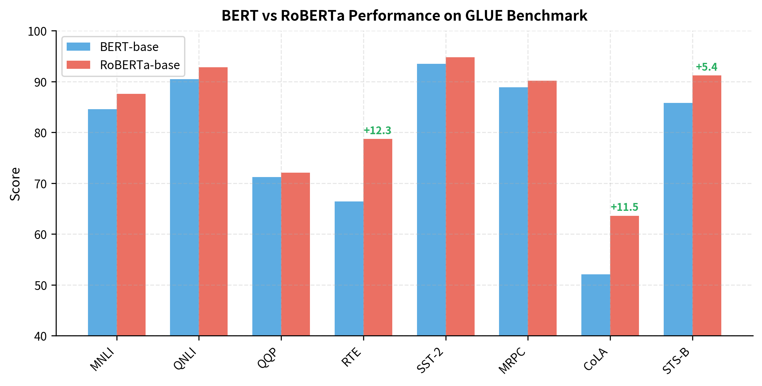
The improvements are striking. RoBERTa gains over 10 points on RTE, over 11 points on CoLA, and 5+ points on STS-B. These aren't marginal improvements; they represent meaningful capability differences. And all of this comes from training changes, not architectural innovations.

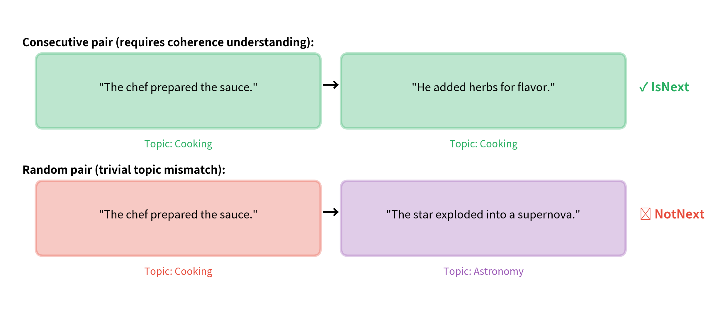
BERT was trained with two objectives: Masked Language Modeling (MLM) and Next Sentence Prediction (NSP). The NSP task classifies whether two sentences appear consecutively in the original text or are randomly paired. The intuition was that NSP would help the model understand document-level coherence.

RoBERTa's first major finding was that NSP hurts more than it helps. When the researchers trained BERT with MLM only, removing NSP entirely, performance improved on most downstream tasks.

Why would a seemingly useful objective hurt performance? Several factors contribute:

The NSP task is too easy. Randomly sampled sentences often come from completely different documents and topics. The model can solve NSP by detecting topic shifts rather than learning genuine discourse coherence. A sentence about cooking paired with one about astrophysics is trivially distinguishable without understanding narrative flow.

NSP constrains the input format. BERT's NSP training requires inputs to be sentence pairs, typically short. This prevents the model from seeing longer contiguous passages that might teach it more about extended context and document structure.

NSP dilutes the learning signal. Half the model's training updates come from a task that may not transfer well to downstream applications. Those gradients could instead strengthen the MLM objective.

The RoBERTa paper tested several input formats:

The DOC-SENTENCES format performed best. Models trained without NSP and on longer contiguous passages learn better representations. The takeaway: NSP was a red herring. The simple MLM objective on longer contexts works better.

BERT used static masking: the training data was preprocessed once, with masks applied and saved. Each training example always had the same tokens masked, even across multiple epochs. This limited the diversity of training signal.

RoBERTa introduced dynamic masking: masks are generated on-the-fly during training. Each time the model sees a sequence, different tokens are masked. Over multiple epochs, the model sees the same underlying text with many different masking patterns.

Let's visualize the difference over multiple training epochs:

With static masking, the model sees identical inputs across all epochs. With dynamic masking, each epoch presents new challenges. Position 3 might be masked in epoch 1, positions 2 and 5 in epoch 2, and so on. This multiplies the effective training diversity without requiring more data.

The empirical benefit of dynamic masking is modest but consistent. The RoBERTa paper found it slightly improves or matches static masking across all benchmarks. More importantly, it's simpler: there's no need to preprocess and store multiple masked versions of the data. Masking happens during training, reducing storage requirements and preprocessing complexity.

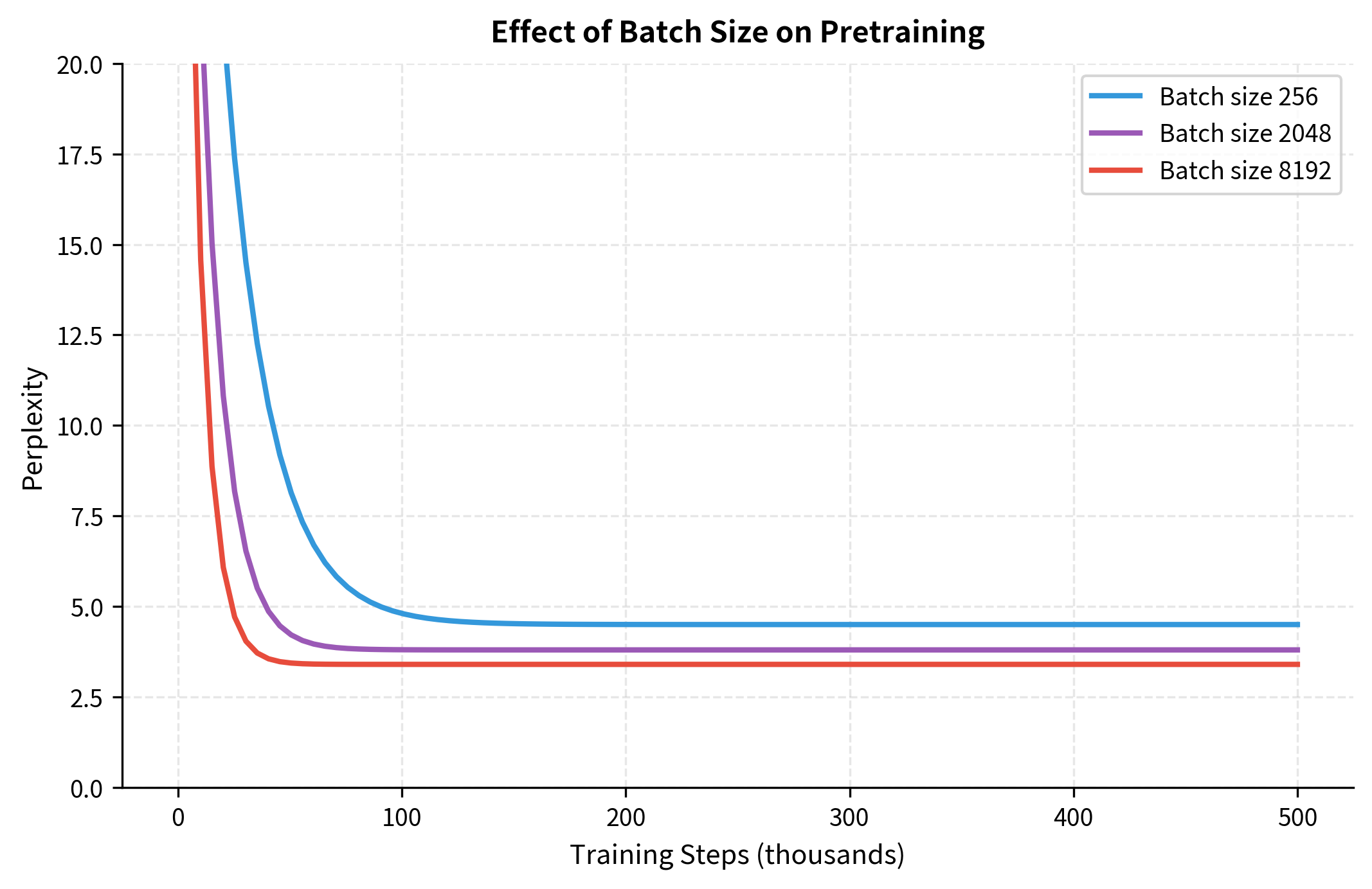
BERT-base was trained with a batch size of 256 sequences. RoBERTa found that much larger batches improve both training stability and final performance. The key insight is that larger batches provide better gradient estimates, especially important for MLM where only 15% of tokens contribute to each update.

Why do larger batches help MLM specifically? Consider the gradient signal per update:

• With batch size 256 and 15% masking, each update aggregates gradients from roughly $256 \times 512 \times 0.15 \approx 19,700$ masked tokens
• With batch size 8192, this grows to $8192 \times 512 \times 0.15 \approx 629,000$ masked tokens

The larger gradient estimates are less noisy, allowing the optimizer to take more confident steps. This translates to faster convergence and better final performance.

RoBERTa used batch sizes up to 8192 sequences. To maintain the same number of parameter updates, larger batches require adjusting the learning rate. The linear scaling rule suggests multiplying the learning rate by the batch size increase factor, though warmup and careful tuning remain important.

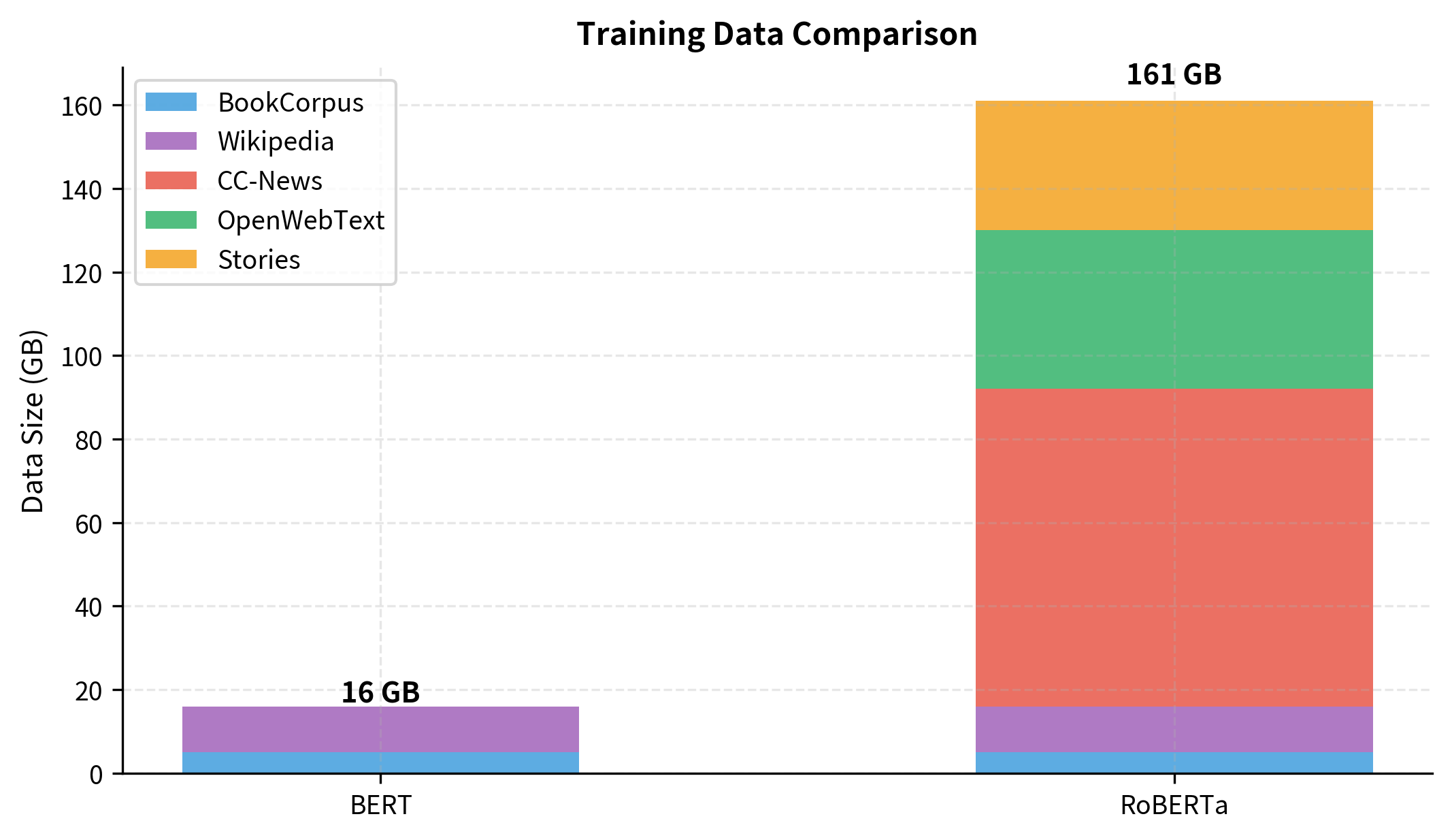
BERT was trained on BookCorpus (800M words) and English Wikipedia (2,500M words), totaling about 16GB of uncompressed text. RoBERTa expanded this substantially by adding three more datasets:

• CC-News: 76GB of news articles crawled from Common Crawl
• OpenWebText: 38GB of web content from Reddit-linked URLs
• Stories: 31GB of story-like content from Common Crawl

The combined dataset is roughly 160GB, ten times larger than BERT's original training data. But data alone isn't enough. RoBERTa also trained for significantly more steps.

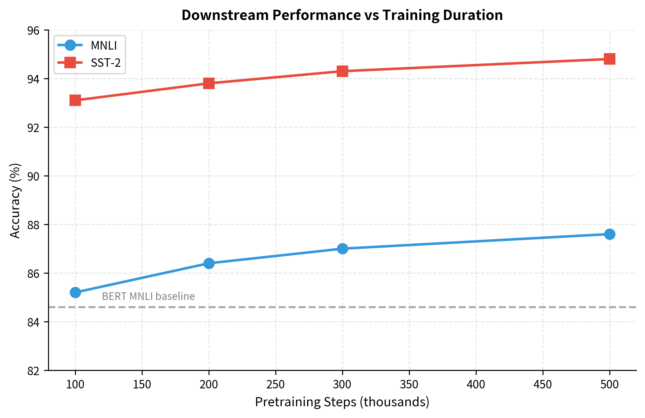
The paper systematically varied training duration to understand its impact. They found that longer training consistently improved performance, even past the point where loss on the training data plateaued. This suggests that the model continues to learn useful representations even when the pretraining objective stops improving.

Let's consolidate all the changes that transform BERT into RoBERTa:

The RoBERTa paper carefully ablated each change to understand its individual contribution. The following visualization shows how performance on MNLI improves as each modification is applied cumulatively:

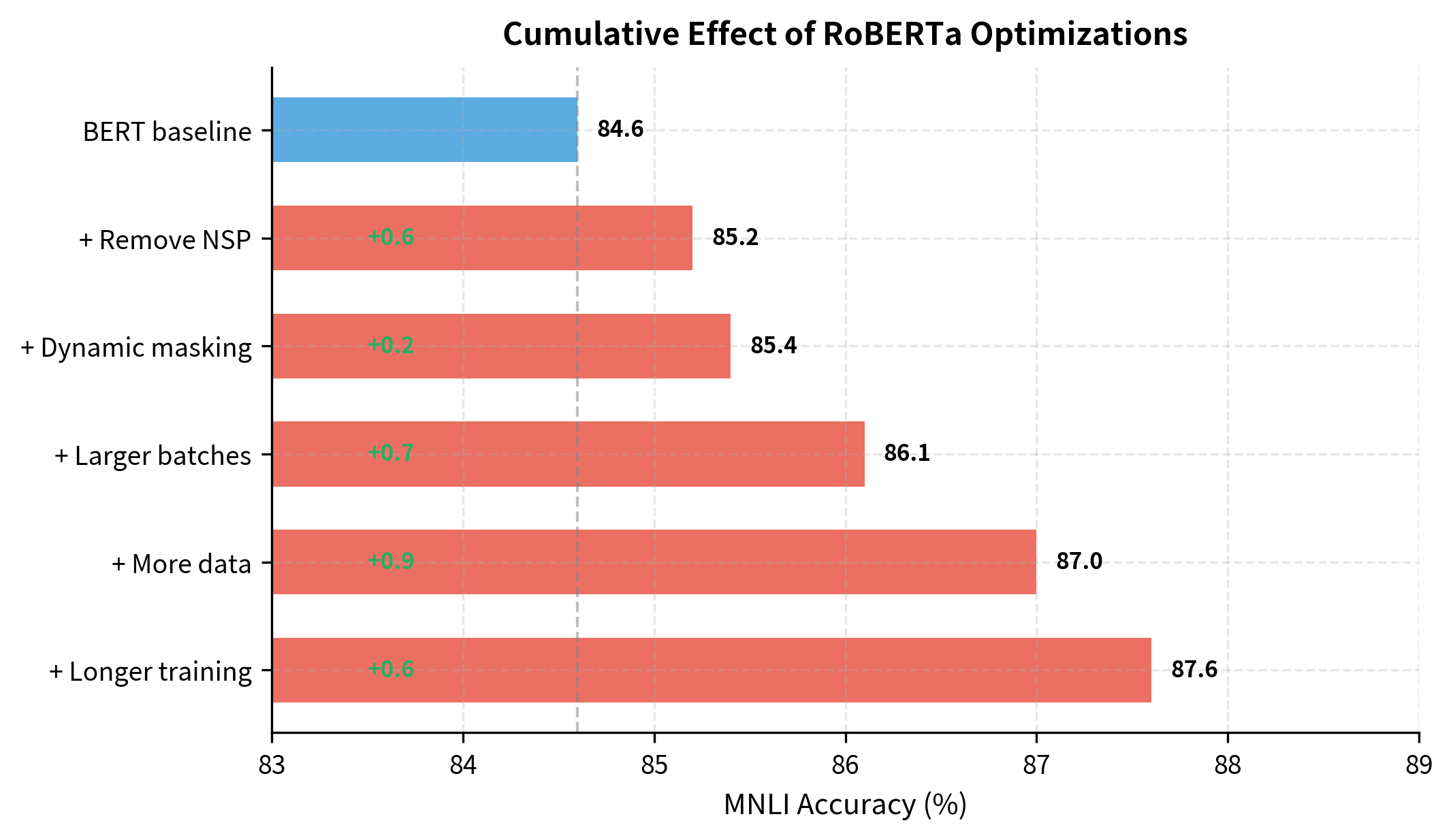
Each optimization contributes to the final result. Removing NSP provides a small but consistent gain. Dynamic masking adds marginally more. The largest improvements come from scaling: larger batches stabilize gradients, more data provides diverse training signal, and longer training allows the model to fully absorb this information. Together, these changes yield a 3-point improvement, a substantial gain for a model with identical architecture.

Notice that RoBERTa uses fewer training steps than BERT. This might seem contradictory to "training longer," but the larger batch size means each step processes far more data. The total number of tokens seen is about 10x higher in RoBERTa despite fewer steps.

RoBERTa sees roughly 16 times more tokens than BERT. Combined with the architectural simplification of removing NSP and the improved signal from dynamic masking, this massive increase in training scale produces substantially better representations.

Let's implement the key differences between BERT and RoBERTa training. We'll focus on the data loading and masking pipeline, which captures the most important changes.

Now let's implement the full-sentences input format that RoBERTa uses instead of sentence pairs:

The first example starts with the [CLS] token (ID 0), contains packed text from the documents, and would end with [SEP] (ID 2). The key insight is that RoBERTa's input format is simpler than BERT's. No segment embeddings needed for NSP, no alternating sentence A and B. Just pack as much contiguous text as possible and apply MLM.

Let's put together a minimal training loop that highlights the differences:

The RoBERTa training step is cleaner. No NSP labels to prepare, no segment embeddings to track, no secondary loss to balance. This simplicity makes training easier to debug and scale.

In practice, you'll likely use RoBERTa through the Hugging Face transformers library rather than training from scratch. Here's how to load and use it:

RoBERTa correctly predicts "Paris" with high confidence. The model has learned rich representations of factual knowledge through its MLM pretraining.

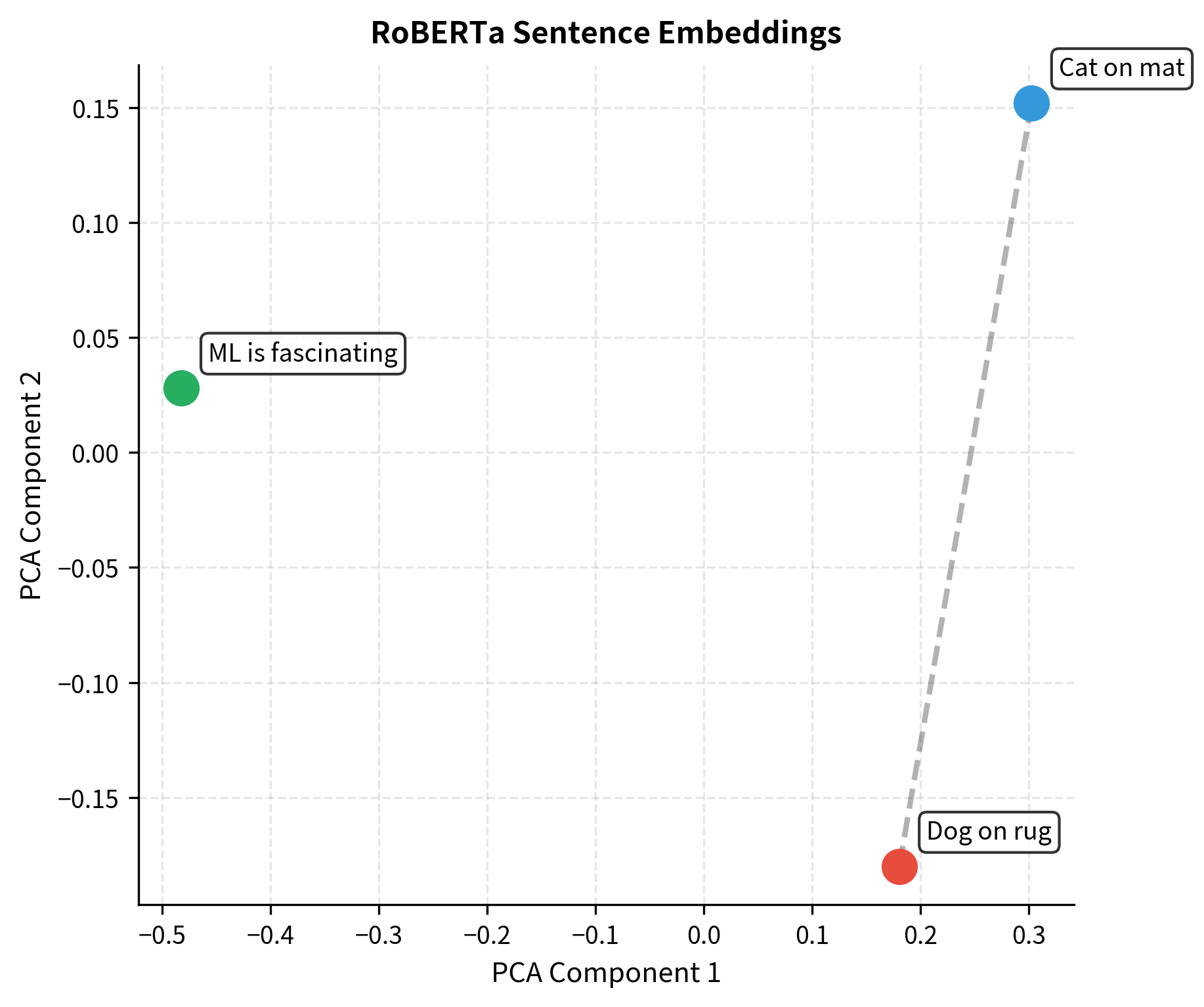
For downstream tasks, you often want the hidden state representations rather than MLM predictions. Here's how to extract them:

The similarities make sense: the two sentences about animals on surfaces are more similar to each other than to the machine learning sentence. RoBERTa's representations capture semantic relationships effectively.

RoBERTa's contribution is both its strength and its limitation. The paper demonstrated that BERT was undertrained, but it did so through brute force: more data, more compute, more time. This isn't a scalable research methodology. Not every lab can replicate the conditions needed to train a model for weeks on 1024 V100 GPUs.

The removal of NSP remains somewhat controversial. While RoBERTa showed that NSP hurts on GLUE benchmarks, some researchers argue that sentence-level objectives matter for tasks requiring cross-sentence reasoning. Models like ALBERT reintroduced sentence-level objectives in modified forms, suggesting the story isn't complete.

RoBERTa also doesn't address MLM's fundamental limitations. The model still cannot generate text autoregressively. It still processes fixed-length sequences. It still requires significant compute for inference. These limitations drove the field toward encoder-decoder models like T5 and decoder-only models like GPT.

Yet RoBERTa's impact was substantial. It established that careful training matters as much as architecture design. It provided a stronger baseline that subsequent papers had to beat. Its open release democratized access to high-quality pretrained models. And it showed that simple, principled improvements often outperform complex architectural changes.

The lesson extends beyond NLP: before proposing new architectures or objectives, ensure existing approaches are properly optimized. Many research "improvements" might be artifacts of undertrained baselines. RoBERTa proved this point emphatically, and the field has been more careful about training protocols ever since.

When implementing or fine-tuning RoBERTa, these parameters most significantly impact performance:

• mask_prob (default: 0.15): Fraction of tokens to mask per sequence. The 15% rate balances training signal strength against context preservation. Higher rates mask more tokens per update but risk destroying too much context for accurate predictions.

• batch_size (RoBERTa default: 8192): Number of sequences per training step. Larger batches provide more stable gradient estimates, particularly important for MLM where only 15% of tokens contribute gradients. Requires proportional learning rate scaling.

• max_seq_len (default: 512): Maximum sequence length. Longer sequences capture more context but require quadratically more memory for attention. RoBERTa packs contiguous text up to this limit.

• vocab_size (RoBERTa: 50265): Size of the BPE vocabulary. RoBERTa uses a 50K vocabulary trained on its larger dataset, slightly larger than BERT's ~30K.

• special_token_ids: Token IDs that should never be masked, including <s> (CLS), </s> (SEP), and <pad>. These tokens serve structural purposes and masking them would disrupt input format.

• learning_rate: Typically 1e-4 to 6e-4 for pretraining. When scaling batch size, apply the linear scaling rule: if you double batch size, double the learning rate (with appropriate warmup).

RoBERTa demonstrated that BERT was undertrained by systematically optimizing its pretraining recipe. The key changes include:

• Removing Next Sentence Prediction: NSP proved to be a hindrance rather than a help. Training on full sentences without NSP produces better representations for downstream tasks.

• Dynamic masking: Generating fresh masks each training step instead of using static masks increases training signal diversity and slightly improves results.

• Larger batch sizes: Training with batch sizes up to 8192 provides more stable gradients, especially important given MLM's sparse 15% masking rate.

• More data and longer training: Expanding training data 10x and processing more total tokens dramatically improves model quality.

• Full-sentence format: Packing contiguous text into sequences without artificial sentence boundaries allows the model to learn from longer coherent contexts.

None of these changes require modifying BERT's architecture. RoBERTa uses the exact same transformer encoder with the exact same hidden dimensions, attention heads, and layer counts. The improvements come entirely from training methodology.

The practical implication is clear: when using pretrained models for NLP tasks, RoBERTa generally outperforms BERT with no additional complexity. Its representations are richer, its downstream performance is higher, and it requires no special handling for sentence pairs. For most applications, RoBERTa is the better starting point for fine-tuning.