

Understand how residual connections solve the vanishing gradient problem in deep networks. Learn the math behind skip connections, gradient highways, residual scaling, and pre-norm vs post-norm configurations.

This article is part of the free-to-read Language AI Handbook
Choose your expertise level to adjust how many terms are explained. Beginners see more tooltips, experts see fewer to maintain reading flow. Hover over underlined terms for instant definitions.
Residual Connections
Deep neural networks learn by stacking layers, with each layer refining the representation from the previous one. In theory, adding more layers should only help: a deeper network can learn anything a shallower network can, plus potentially more complex patterns. In practice, something strange happens. Beyond a certain depth, networks become harder to train. Loss stops decreasing. Accuracy plateaus or even drops.
Residual connections solve this paradox. By adding a simple shortcut that lets information bypass each layer, residual connections transform the optimization landscape. Instead of learning absolute transformations, layers learn small adjustments. Instead of gradients dying across dozens of layers, they flow freely through shortcut paths. This architectural pattern is so effective that it's now standard in virtually every deep learning architecture, from ResNets in computer vision to transformers in NLP.
This chapter explores the mathematics behind residual connections, their interpretation as gradient highways, and their specific role in transformer architectures. We'll also examine the choice between pre-norm and post-norm configurations, which affects training stability in ways that matter for very deep models.
The Deep Network Problem
Before residual connections, training deep networks was notoriously difficult. The culprit is the chain rule of calculus: during backpropagation, gradients are multiplied layer by layer. With many layers, these products either explode or vanish.
Deep networks have more representational capacity than shallow ones, but they're harder to optimize. The gradient signal that guides learning must travel through every layer, and each layer can amplify or diminish it. With dozens of layers, even small per-layer effects compound catastrophically.
Consider a network with layers. During backpropagation, we need to compute how the loss changes with respect to parameters deep in the network. The chain rule tells us to multiply derivatives through each intermediate layer. For parameters in layer , this gradient involves products of Jacobian matrices from all subsequent layers:
where:
- : the loss function we're minimizing (e.g., cross-entropy)
- : parameters (weights and biases) in layer
- : the hidden representation (activation vector) at layer
- : the final output of the network
- : the Jacobian matrix of layer 's transformation, showing how each output dimension depends on each input dimension
- : the product of all Jacobians from layer to the output layer
The critical term is the product of Jacobians. Each Jacobian is a matrix, and we multiply of them together. If each Jacobian has spectral norm (largest singular value) slightly greater than 1, the product grows exponentially. If slightly less than 1, it shrinks exponentially. For example, with spectral norm 0.9 across 50 layers, the gradient shrinks by a factor of , effectively killing the learning signal.
Keeping gradients stable across 50 or 100 layers requires exquisite balance that's nearly impossible to maintain during training.
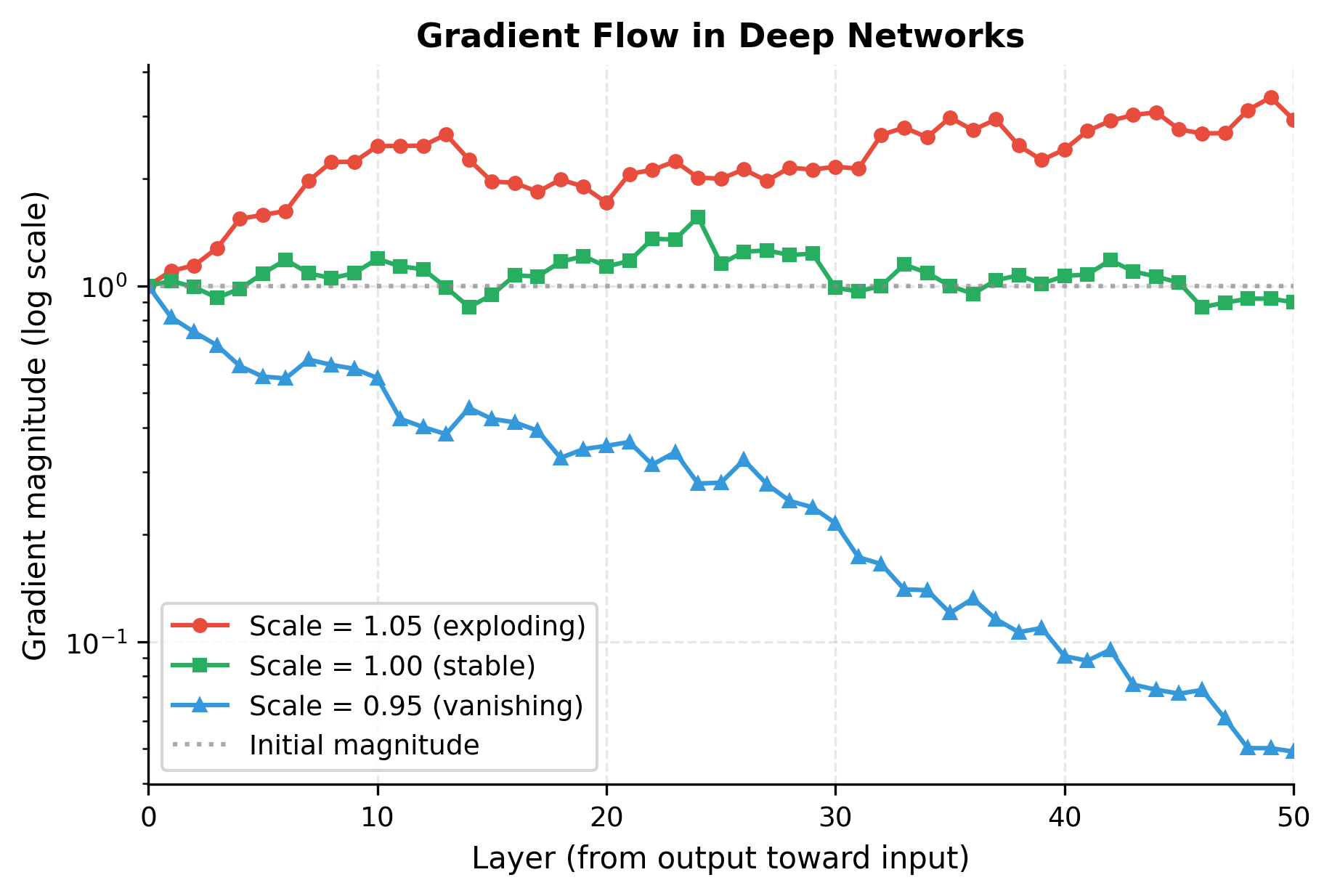
The simulation reveals the challenge. A mere 5% deviation from perfect gradient preservation compounds across 50 layers to produce 10x amplification or 90% attenuation. Real networks with nonlinearities, varying weight magnitudes, and changing activation patterns face even more severe instabilities. Training such networks requires fighting against mathematics.
Why Adding Layers Can Hurt Performance
A counterintuitive phenomenon plagued early deep learning: adding more layers to a well-performing network often decreased accuracy. This wasn't just about training difficulty. Even on training data, deeper networks performed worse than shallower ones.
This violates basic intuition. A 56-layer network should be at least as expressive as a 20-layer network: it could theoretically learn to make the extra 36 layers act as identity mappings, reproducing the shallower network's behavior. Yet empirically, the 56-layer network trains to higher error.
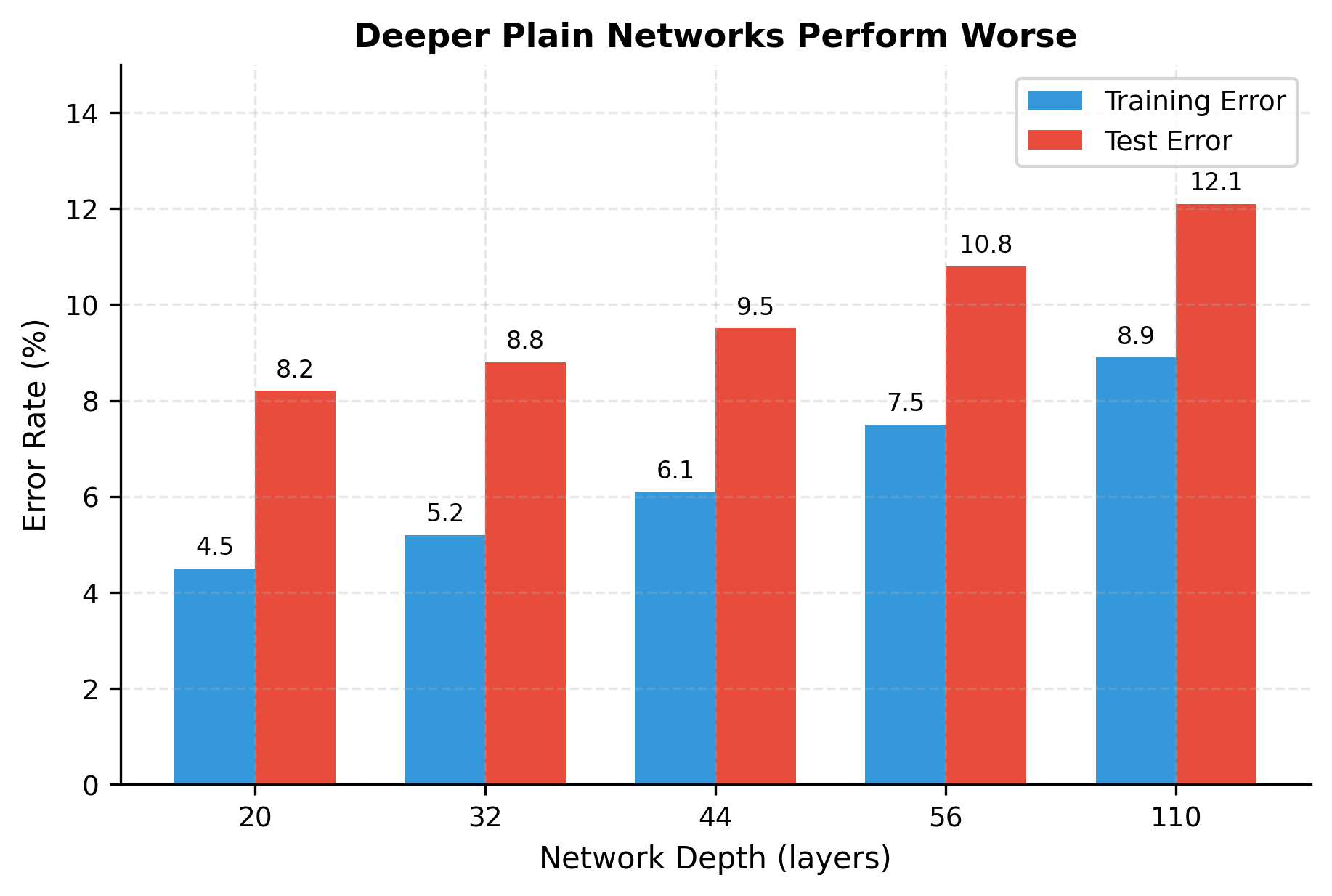
The pattern is unmistakable: deeper plain networks achieve higher error on both training and test sets. If this were overfitting, we'd see low training error and high test error. Instead, both increase monotonically with depth. The optimization itself is failing. The deeper networks simply cannot learn the transformations they theoretically can represent.
The Residual Connection Solution
The degradation problem presents a paradox: deeper networks should be more expressive, yet they perform worse. The solution comes from rethinking what we ask each layer to learn.
Consider a network that already performs well at 20 layers. If we add 10 more layers, the ideal outcome might be for those extra layers to simply pass information through unchanged, effectively becoming identity mappings. But asking a layer to learn through its weights is surprisingly difficult. The layer must coordinate all its parameters to reproduce the input exactly, and any training noise pushes it away from this fragile configuration.
What if, instead of learning the complete transformation, each layer only learned the adjustment to make? This shift in perspective is the key insight behind residual learning.
From Transformations to Adjustments
In a traditional neural network, each layer maps its input to a completely new representation. Given input , the layer computes:
where:
- : the input representation (a vector of activations from the previous layer)
- : the output representation (passed to the next layer)
- : the layer's learned transformation, typically combining linear projections (weights), nonlinearities (like ReLU), and possibly normalization
The layer bears full responsibility for producing from scratch. Every useful feature in the output must be constructed by the learned function .
Now consider what happens if the optimal output is simply the input, unchanged. The layer must learn . This is an identity mapping, and while mathematically simple, it requires precise coordination of weights. Any perturbation during training disrupts this delicate balance.
Residual connections flip this relationship. Instead of learning the output directly, the layer learns only the difference between desired output and input:
where:
- : the residual function, representing only the change the layer should make
- : added directly to form the output (the skip or shortcut connection)
- : equals the input plus whatever adjustment learns
The addition is the skip connection or shortcut. It provides a direct path for the input to flow to the output unchanged. The function now only needs to learn what to add to the input, rather than recreating the input plus modifications.
A residual block computes , where is the transformation learned by the layer and is the input. The layer learns the residual rather than the full mapping. If the optimal transformation is close to identity, the layer only needs to learn small adjustments.
The Identity Mapping Advantage
This reformulation seems minor, just adding a term, but it fundamentally changes the optimization landscape. Consider what each architecture must learn to achieve an identity mapping:
| Architecture | To produce , must learn: | Difficulty |
|---|---|---|
| Traditional | Hard: requires precise weight configuration | |
| Residual | Easy: just set weights to zero |
For the traditional layer, learning identity requires that every weight matrix perfectly reproduces the input. For the residual block, learning identity requires only that , which happens automatically when weights are small or zero. The skip connection handles the identity part for free.
This asymmetry has profound implications:
-
Easy initialization: A residual block initialized with small weights is nearly an identity function, passing information through without disruption.
-
Graceful degradation: If a layer's contribution isn't helpful, it can "turn off" by driving toward zero. The network doesn't lose information because still flows through.
-
Additive refinement: Each layer adds information rather than replacing it. The network builds up its representation incrementally, with each layer contributing what it can.
Demonstrating the Difference
Let's see this principle in action. We'll create two blocks, one traditional and one residual, and observe how they behave when initialized with small weights.
The two classes are nearly identical, differing only in their final line: the plain block returns out while the residual block returns x + residual. This single change, adding the input back, creates the skip connection.
Now we'll test what happens when the output layer is initialized to zero, simulating a layer that hasn't yet learned to contribute:
The results reveal the fundamental difference. The plain block, with its output layer zeroed, produces output with near-zero norm. It has destroyed the input signal entirely. The residual block, in contrast, produces output identical to its input. The skip connection preserves information perfectly when the learned function contributes nothing.
This behavior at initialization cascades through deep networks. Stack 50 plain blocks with zero output layers, and the signal is completely lost. Stack 50 residual blocks with zero output layers, and the input passes through unchanged. As training progresses, each layer can gradually "turn on" its residual contribution without ever disrupting the signal flow.
The Gradient Highway Interpretation
The forward pass benefits of residual connections, preserving information and enabling identity mappings, are compelling. But the real power emerges during backpropagation. Skip connections don't just help information flow forward; they create express lanes for gradients to flow backward.
To understand why this matters, recall the vanishing gradient problem from earlier. In plain networks, gradients must traverse every layer's Jacobian matrix, and even slight attenuation at each layer compounds to near-zero gradients deep in the network. Residual connections fundamentally change this dynamic.
Unrolling the Residual Network
Consider a deep network with residual blocks. Let be the network input and be the output of block . Each block computes:
where:
- : the input to block (output of block )
- : the output of block
- : the residual function for block (the learned transformation, excluding the skip connection)
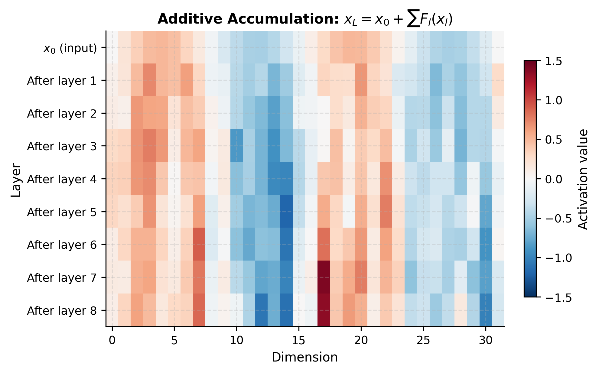
Unlike traditional layers that chain together as compositions , residual blocks have an additive structure. We can unroll this recurrence to see the elegant form it takes:
This formulation reveals something remarkable: the output is the sum of the original input and all intermediate residuals. The input isn't transformed through a chain of compositions. Instead, it's preserved and augmented. Each layer contributes additively rather than multiplicatively.
The Gradient Decomposition
Now we trace gradients backward. We want to compute how the loss changes with respect to an early representation . The chain rule gives:
where:
- : the gradient at the output layer (computed from the loss)
- : how changes in affect the final output
The critical question is: what is ? From the unrolled formulation , we differentiate with respect to :
where:
- The 1 comes from the direct path: contributes to through the chain of skip connections ()
- The sum captures indirect contributions through the residual functions
This decomposition is the heart of residual learning. The gradient splits into two components:
-
Direct path (the "1"): Gradients flow directly through skip connections, completely bypassing all layer transformations. This path always contributes exactly 1 to the gradient magnitude.
-
Residual path (the sum): Gradients flow through the learned functions , just as they would in a plain network. This path can vanish, explode, or behave unpredictably.
The key insight: even if the residual path completely vanishes (all ), the gradient still maintains magnitude 1 through the identity path. The skip connection guarantees a floor on gradient magnitude.
Seeing the Gradient Highway in Action
Let's simulate this gradient decomposition to see how the two paths behave as we go deeper into the network:
We simulate 20 layers where the residual path loses half its gradient at each layer (a 50% attenuation, more optimistic than many real networks). The direct path, by design, contributes exactly 1.0 at every layer:
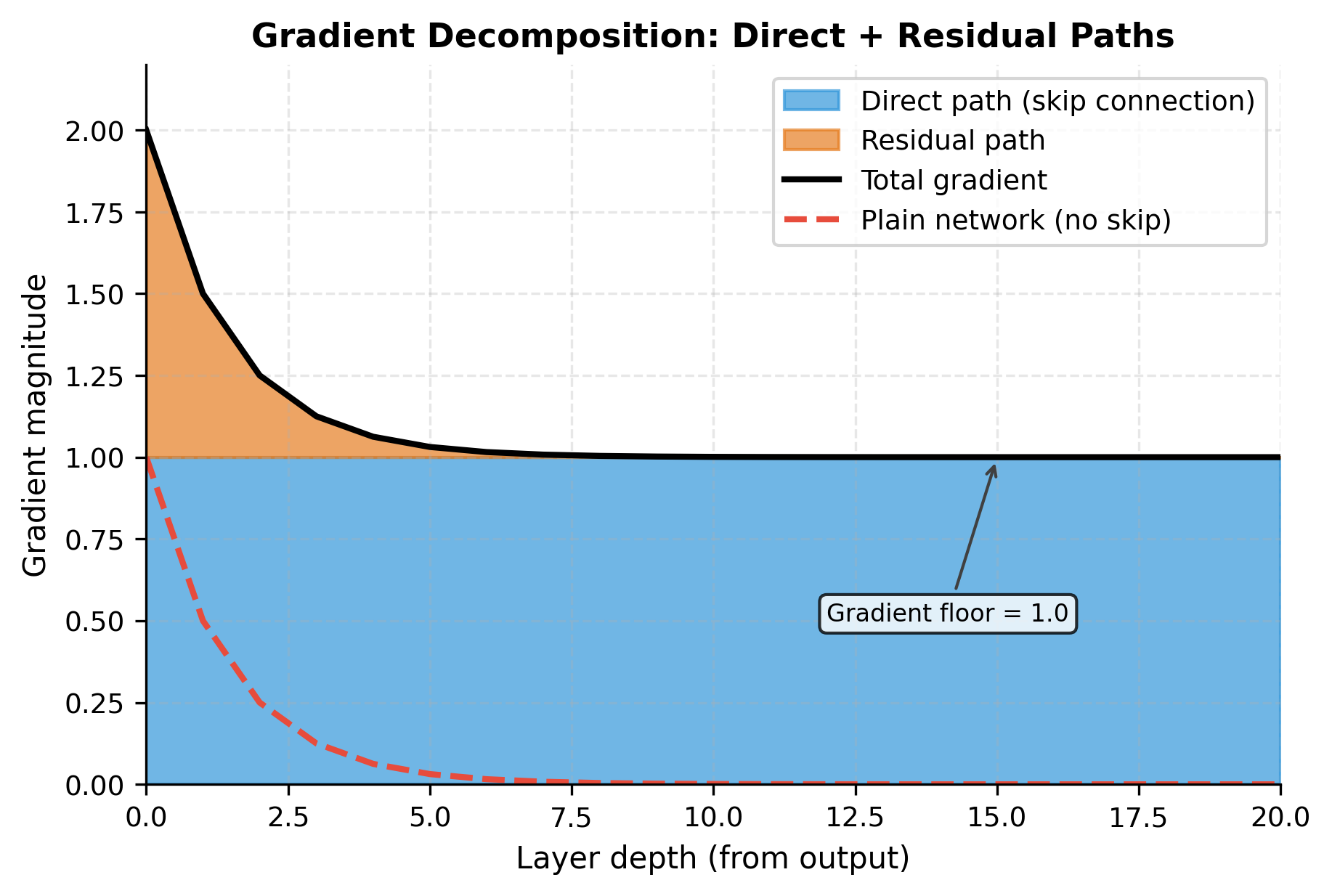
The table reveals the mechanism with striking clarity. The direct path column shows unwavering 1.0 values at every depth. This is the gradient highway, completely unaffected by layer count. Meanwhile, the residual path decays exponentially: by layer 16, it contributes only 0.000008 to the gradient, essentially vanishing as it would in a plain network.
But here's the crucial difference from plain networks: the total gradient never drops below 1.0. In a 20-layer plain network with 50% gradient attenuation per layer, the gradient would be , effectively zero. In the residual network, it's 1.000001. The skip connection provides a floor that prevents gradients from vanishing entirely.
Visualizing the Gradient Highway
The term "gradient highway" captures this behavior perfectly. Think of a city's road network: local streets pass through many intersections, each one potentially causing delays or blockages. An expressway bypasses these intersections entirely, providing guaranteed throughput regardless of local traffic conditions. Skip connections serve the same purpose for gradients. They bypass the potentially problematic layer transformations, providing guaranteed gradient flow to early parameters.
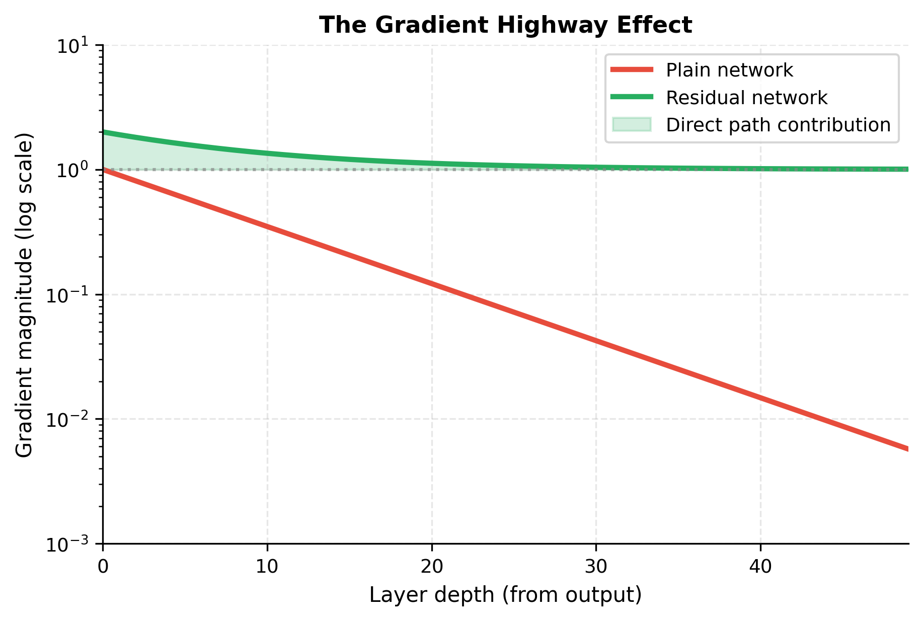
The visualization captures the essential difference. In plain networks, gradients decay exponentially. In residual networks, the direct path provides a floor: gradients never fall below 1.0 (plus whatever the residual path contributes). This guaranteed minimum gradient flow is why residual networks can train effectively at depths that would be impossible for plain networks.
Residual Connections in Transformers
Having established why residual connections work in general, we now turn to their specific application in transformers. The transformer architecture relies heavily on residual connections, not as an optional enhancement, but as a fundamental design principle that makes training possible.
A transformer encoder or decoder consists of stacked identical blocks. Each block contains two distinct operations: multi-head self-attention (which lets tokens gather information from each other) and a position-wise feed-forward network (which processes each token independently). Without residual connections, stacking 12, 24, or 96 of these blocks would be impossible to train. With them, modern language models routinely use such depths.
The Transformer Block Pattern
A standard transformer block processes input through two sub-layers, each wrapped with its own residual connection. The computation proceeds as:
where:
- : input to the transformer block, with tokens and -dimensional embeddings
- : the attention sub-layer output, same shape as
- : intermediate representation after the first residual addition
- : the feed-forward sub-layer output, same shape as
- : final block output, passed to the next transformer block
Each addition () represents a skip connection. Notice the interpretive power this structure provides:
-
Attention as adjustment: The attention sub-layer doesn't produce a completely new representation; it learns what context-aware information to add to each token based on other positions in the sequence.
-
FFN as refinement: The feed-forward network learns what position-wise transformations to add to the post-attention representation, processing each token independently.
-
Graceful bypass: If either sub-layer's contribution isn't helpful for a particular input, it can learn to produce near-zero output. The information flows through unchanged via the skip connection.
This framing helps understand what transformers actually learn: not arbitrary transformations at each layer, but successive refinements to a representation that remains connected to the original input.
The block processes a batch of 4 sequences, each with 16 tokens and 512-dimensional embeddings. The output maintains the same shape, a requirement for residual connections to work since the addition requires matching dimensions. With over 6 million parameters split between attention and FFN, each sub-layer contributes its learned adjustments through the residual pattern x + SubLayer(x).
Why Every Sub-Layer Gets a Residual
You might wonder: why not just one residual connection per transformer block, wrapping both attention and FFN together? The answer relates to optimization stability and gradient flow.
With residual connections around each sub-layer:
- Gradients have two "highways" per block: one bypassing attention, one bypassing FFN
- Each sub-layer can be trained somewhat independently
- The network can easily learn to skip either sub-layer if it's not helpful
With a single residual per block:
- Gradients must flow through both attention and FFN or bypass both
- Harder to learn that attention is useful but FFN isn't (or vice versa)
- Effectively half as many gradient highways
The empirical result is that per-sub-layer residuals train more stably and achieve better final performance, especially in deep networks.
Residual Scaling
Residual connections solve the vanishing gradient problem beautifully, but they introduce a subtler issue in very deep networks. Recall the unrolled form: . We're summing residuals. If each residual has similar magnitude, the sum grows with depth.
For a 12-layer transformer, this growth is manageable. For a 96-layer model, summing residuals can cause the representation magnitude to explode, destabilizing training even though gradients flow well. The network needs a mechanism to control this accumulation.
The Scaling Factor
Residual scaling dampens each residual contribution before adding it to the skip path. Instead of , we compute:
where:
- : a scaling factor, typically
- : the residual function output
- : the dampened residual, smaller in magnitude than the original
The design question is: what value should take? Several strategies have proven effective:
-
Fixed scaling: or similar constant, chosen empirically. Simple and effective for moderately deep networks.
-
Depth-dependent: where is total layers. This ensures the variance of the sum stays bounded as depth increases, based on the statistics of summing independent random variables.
-
Learned: as a trainable parameter per layer, allowing the network to discover appropriate scaling during training. More flexible but adds parameters.
Each approach reduces each layer's contribution, preventing the sum of residuals from growing unboundedly. Importantly, scaling doesn't hurt gradient flow: the gradient still flows through the unscaled skip connection, maintaining the gradient highway effect.
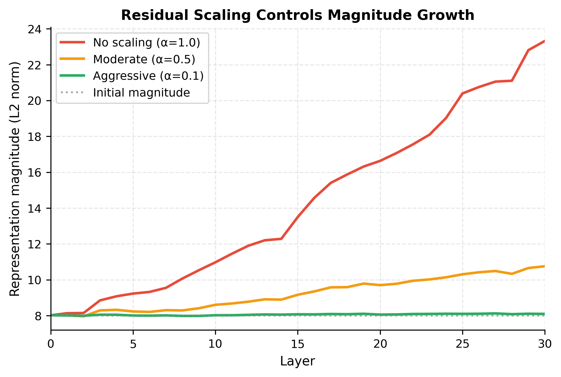
The visualization reveals the trade-off clearly. Without scaling (α = 1.0), the representation magnitude grows steadily as each layer adds its full residual contribution. The growth appears roughly linear because we're adding vectors of similar magnitude. With moderate scaling (α = 0.5), growth slows substantially. With aggressive scaling (α = 0.1), the magnitude stays nearly constant. Each layer contributes so little that the sum barely increases.
The optimal choice balances two concerns: too little scaling allows magnitude explosion in very deep networks, while too much scaling limits each layer's expressive contribution. A depth-dependent rule like provides automatic balance: deeper networks use smaller scaling factors.
ReZero: Learning to "Turn On" Layers
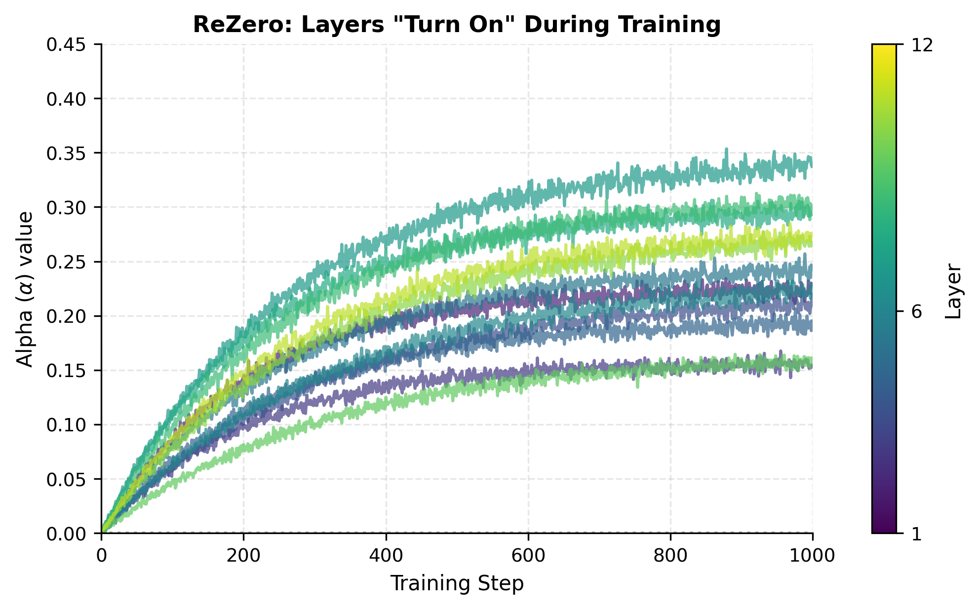
The fixed and depth-dependent scaling approaches require choosing before training. But what if the network could discover the right scaling for each layer on its own? The ReZero approach takes this idea to its logical extreme: initialize every scaling factor to zero, and let the network learn when and how much to "turn on" each layer.
where:
- : a learnable scalar parameter, initialized to 0
- : at the start of training, , so exactly
At initialization, every residual block is exactly an identity mapping, not approximately, but perfectly. The entire network is just a pass-through. As training progresses, gradient descent increases values where the residual function provides useful contributions. Layers that aren't helpful can keep near zero.
This approach offers elegant properties:
- Perfect identity initialization: No approximation errors, no disruption to signal flow at the start of training
- Layer-specific adaptation: Important layers develop larger values; less useful layers remain suppressed
- Automatic depth scaling: In very deep networks, the collective values naturally stay small enough to prevent magnitude explosion
The output confirms that ReZero works as intended. With alpha initialized to exactly zero, the block is a perfect identity function: input and output are identical, not merely close. The residual function still computes something (it has weights and activations), but its contribution is completely suppressed by the zero multiplier.
During training, gradient descent will increase alpha when doing so reduces the loss. Early in training, alpha values remain small, keeping the network close to identity. As the residual functions learn useful transformations, their alpha values grow to let those transformations contribute. This creates a natural curriculum: the network starts simple and gradually increases complexity.
Pre-Norm vs Post-Norm Residuals
We've established that residual connections enable deep network training through gradient highways. But there's a subtle design choice that significantly affects training dynamics: where do you place layer normalization relative to the residual addition?
Layer normalization is essential for stable training. It prevents activations from exploding or vanishing by normalizing to zero mean and unit variance. But its placement interacts with the skip connection in ways that matter for very deep networks. The two configurations are post-norm (the original transformer design) and pre-norm (now the dominant choice for large models).
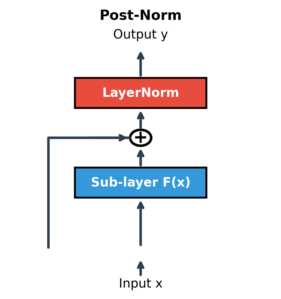
Post-Norm: The Original Configuration
The original "Attention Is All You Need" paper uses post-norm, where normalization comes after the residual addition:
where:
- : the input to the block
- : the sub-layer output (e.g., attention or FFN)
- : the residual sum
- : layer normalization applied to the combined result
- : the final block output, normalized
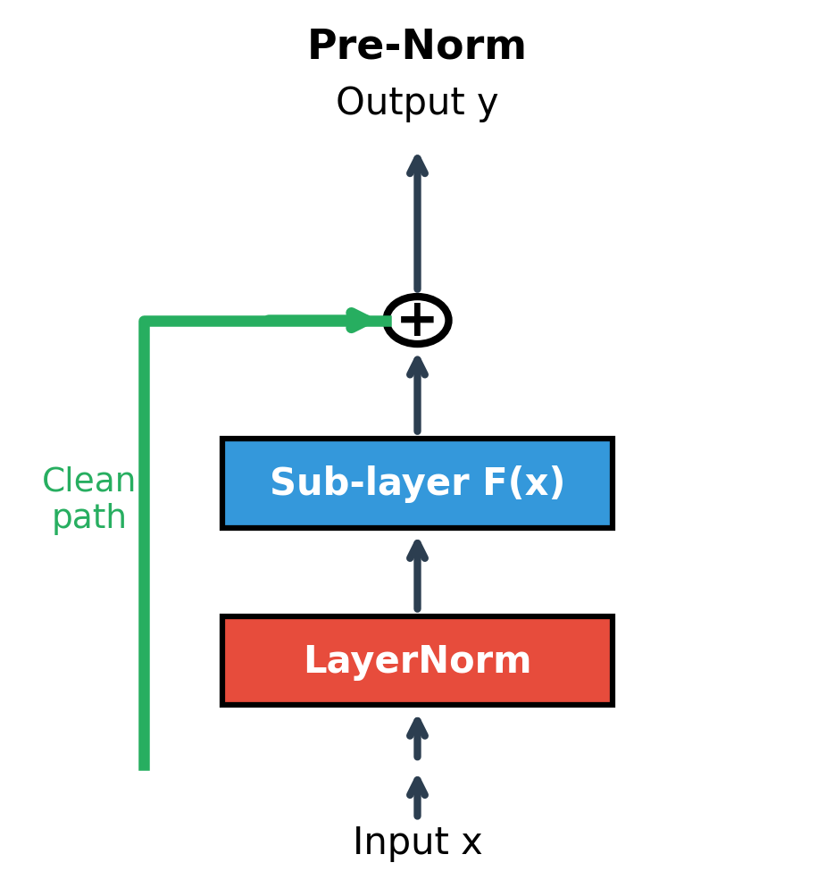
Pre-Norm: The Modern Default
Pre-norm rearranges the components, applying normalization before the sub-layer rather than after the residual addition:
where:
- : normalization applied to the input before the sub-layer
- : the sub-layer operates on normalized input
- : the original input, added directly (not normalized in the skip path)
- : the output, combining raw input with transformed normalized input
This rearrangement might seem cosmetic, but it has a crucial consequence for gradient flow. In post-norm, gradients flowing through the skip connection must pass through the LayerNorm operation, where they're multiplied by the normalization's derivative. In pre-norm, the skip path is completely clean: the term passes gradients backward without any modification.
The pure gradient highway we derived earlier, where the direct path contributes exactly 1 to the gradient, only holds perfectly for pre-norm. Post-norm introduces the normalization's Jacobian into the skip path, which can amplify or attenuate gradients depending on the input statistics.
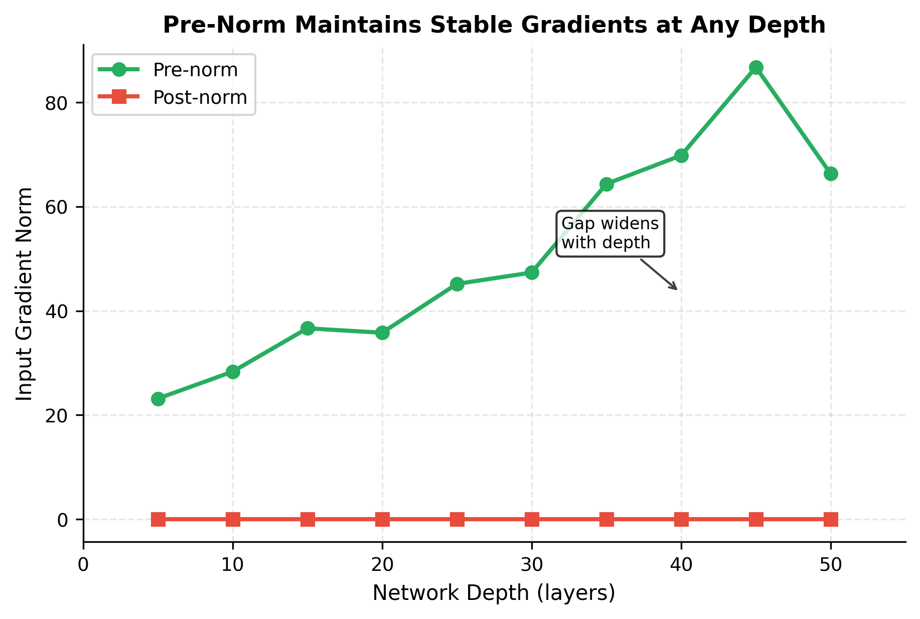
The gradient norm comparison quantifies what the theory predicts. Pre-norm maintains substantially stronger gradients at the input layer after passing through 20 blocks. The ratio between them indicates that post-norm's normalization operations in the skip path attenuate the gradient signal.
For a 20-layer network, this difference is noticeable but perhaps manageable. For a 96-layer model like GPT-3, the gap compounds dramatically. Pre-norm's clean gradient path becomes essential for stable training at that scale.
Training Stability in Practice
The gradient analysis translates directly to practical training differences. Pre-norm transformers are more stable and forgiving during training, especially in challenging regimes:
-
Very deep networks (50+ layers): The cumulative effect of normalization Jacobians in post-norm's skip path compounds with depth. Pre-norm avoids this entirely.
-
Large learning rates: Post-norm requires more careful learning rate tuning because gradient magnitudes are less predictable. Pre-norm tolerates larger learning rates.
-
Reduced warmup schedules: Post-norm typically needs extended warmup periods to avoid early training instabilities. Pre-norm can often skip or shorten warmup.
The mathematical reason is clear: with pre-norm, the skip connection contributes exactly to the gradient at any earlier layer, with no modification and no layer-dependent scaling. With post-norm, this contribution is modulated by the chain of normalization derivatives, introducing variance that can destabilize training.
When to Use Each Configuration
The choice between pre-norm and post-norm depends on your specific situation:
Use Pre-Norm when:
- Training very deep transformers (24+ layers)
- You want faster training convergence
- Stability is more important than squeezing out final performance
- Using larger learning rates or shorter warmup schedules
Use Post-Norm when:
- Fine-tuning pre-trained models that used post-norm
- Willing to use careful learning rate scheduling and warmup
- Optimizing for final quality over training convenience
- Working with shallower networks where stability is less critical
Modern large language models predominantly use pre-norm due to its training stability at scale. GPT-2, GPT-3, LLaMA, and many other recent models adopt pre-norm configurations.
Practical Implementation
Having covered the theory (residual learning, gradient highways, scaling, and normalization placement), we now synthesize everything into a practical implementation. The following code creates a flexible residual block that supports all the variants we've discussed: pre-norm or post-norm configuration, fixed or learned scaling, and ReZero initialization.
The output statistics reveal each configuration's character. Pre-norm and post-norm, both with scale 1.0, transform the input substantially. Notice how the output statistics differ from input. The key difference between them appears in the output distribution: post-norm produces output with statistics closer to zero mean and unit variance (the normalization's effect on the final output), while pre-norm allows more drift.
ReZero behaves distinctly: with scale 0.0, input and output are identical. The residual function computes something, but the zero multiplier suppresses it completely. This is exactly the "perfect identity initialization" property: at the start of training, before alpha increases, ReZero blocks pass information through unchanged.
Deep Network Test
The theoretical benefits of residual connections should manifest in concrete, measurable ways when we build deep networks. Let's construct 30-layer networks with and without residual connections and compare their gradient flow characteristics:
The comparison reveals why residual connections have become ubiquitous in deep learning. At 30 layers of depth, the residual network maintains healthy gradient and output norms. The training signal reaches early parameters with sufficient magnitude to drive meaningful updates. The plain network shows different behavior in its gradient magnitudes, a sign of the compounding effects we analyzed earlier.
This gap widens dramatically with depth. At 50 layers, plain networks become nearly untrainable. At 100 layers, they're hopeless. Residual networks, in contrast, scale gracefully: models with 96, 128, or even 1000+ layers train successfully when equipped with skip connections. This scalability is why every major deep learning architecture since 2015, from ResNets to transformers to diffusion models, incorporates residual connections as a foundational element.
Limitations and Trade-offs
Residual connections have proven remarkably effective, so much so that they're essentially mandatory for deep networks. But no architectural choice is without trade-offs. Understanding the limitations helps make informed design decisions.
Memory Overhead
The skip connection requires storing the input until the residual is computed, so they can be added. In a single block, this is trivial. In a deep network during training, it accumulates:
- Plain networks: Store only the current layer's activations (can discard earlier layers)
- Residual networks: Store input to each block until the addition completes
For training with large batch sizes and long sequences, this memory overhead becomes significant. A 32-layer transformer processing 2048-token sequences might need to store 32 copies of the activation tensor for the residual additions alone. Techniques like gradient checkpointing help by recomputing some activations during the backward pass instead of storing them, trading compute for memory.
Architectural Constraints
The residual formulation imposes a fundamental constraint: and must have matching dimensions for the addition to be valid. In transformers, this is straightforward because the hidden dimension stays constant throughout. But in convolutional networks or architectures that change dimensionality, this creates design challenges.
When dimensions must change (e.g., increasing channels, reducing spatial resolution, or transitioning between embedding sizes), you need projection shortcuts:
where:
- : a learned projection matrix of shape that maps input dimension to output dimension
- : the projected input, now matching the dimension of
- : the residual transformation, which outputs vectors of dimension
Projection shortcuts work, but they sacrifice some benefits. The gradient through is multiplied by , reintroducing potential gradient scaling issues. The skip path is no longer "free": it adds parameters, computation, and a transformation that can amplify or attenuate gradients. This is why transformer architectures prefer to maintain constant dimensions throughout, using the simpler formulation everywhere.
The Identity Plateau Problem
The ease of learning identity mappings, a key feature of residual connections, can become a bug. If the optimization finds a local minimum where for many layers, the network effectively collapses to a much shallower architecture. The layers exist and consume memory, but they contribute nothing.
This "identity plateau" isn't catastrophic (the network still functions), but it fails to utilize the model's full capacity. You've paid for 96 layers but are effectively using 20. Careful initialization, appropriate learning rates, and normalization help avoid this plateau, as does training long enough for gradients to "turn on" dormant layers.
Despite these limitations, residual connections have become indispensable. The benefits (stable gradient flow, trainable depth, additive representation refinement) far outweigh the costs. Any serious deep learning practitioner will encounter residual connections repeatedly; understanding their mechanics is foundational knowledge.
Summary
Residual connections enable training of very deep neural networks by providing direct paths for information and gradients to flow. The core insight is simple: instead of learning transformations directly, layers learn adjustments to an identity baseline. This chapter covered the key concepts and their practical implications.
Key takeaways:
-
The depth problem: Without residual connections, gradients in deep networks either explode or vanish exponentially with depth, making optimization impossible.
-
Residual learning: The formulation lets layers learn residuals (adjustments) rather than full transformations. Identity mappings become trivial, removing a major optimization barrier.
-
Gradient highways: Skip connections provide direct paths for gradient flow. Even if layer gradients vanish, gradients through the skip path maintain a constant magnitude of 1.0.
-
Transformer pattern: Each transformer sub-layer (attention and FFN) is wrapped with its own residual connection. This provides multiple gradient highways per block and allows selective use of each sub-layer.
-
Residual scaling: For very deep networks, scaling residuals by (or learning from zero) prevents representation magnitude from growing unboundedly.
-
Pre-norm vs post-norm: Pre-norm places normalization before the sub-layer, keeping the skip path clean. It's more stable for deep networks and is the modern default. Post-norm was the original configuration and can achieve slightly better final performance with careful training.
Residual connections transformed deep learning from an art of careful initialization and shallow architectures into a science of stacking many simple blocks. Every major architecture since 2015, from ResNets to transformers to diffusion models, builds on this foundation.
Key Parameters
When implementing residual connections in neural networks, several key parameters control their behavior and training dynamics:
-
scale (): The residual scaling factor that multiplies before adding to the skip path. Values less than 1.0 dampen residual contributions, preventing magnitude explosion in very deep networks. Common values range from 0.1 to 1.0, with (where is total layers) providing depth-adaptive scaling.
-
norm_position: Controls whether layer normalization is applied before the sub-layer (pre-norm) or after the residual addition (post-norm). Pre-norm provides cleaner gradient flow and is preferred for deep networks (24+ layers). Post-norm was the original transformer configuration and may achieve marginally better final performance with careful training.
-
rezero: When enabled, initializes the scaling factor to zero, making each block an exact identity function at initialization. The network learns appropriate scaling during training. This eliminates approximation errors at initialization and can speed up early training.
-
dim: The hidden dimension of the residual block. Must match between input and output for the addition to be valid. When dimensions change, projection shortcuts are required.
-
expansion_factor: In feed-forward networks within transformers, this controls the ratio between inner dimension and model dimension. Typical value is 4, meaning .
For transformer implementations in PyTorch, these parameters interact with nn.LayerNorm and nn.MultiheadAttention. The choice between pre-norm and post-norm affects the placement of LayerNorm calls, while residual scaling can be implemented as a learnable nn.Parameter or a fixed constant multiplier.

Comments