Transformer Architecture Hyperparameters: Depth, Width, Heads & FFN Guide

Building a transformer is like designing a building: you must decide how tall to make it, how wide each floor should be, and how to allocate space between different rooms. These architectural decisions, the hyperparameters of transformer design, determine everything from model capacity to training dynamics to inference speed. Get them wrong, and your model might train slowly, underperform, or consume excessive memory. Get them right, and you unlock the performance that makes transformers so powerful.

This chapter explores the key architectural hyperparameters: model depth versus width trade-offs, the number of attention heads, feed-forward network dimensions, and how these choices interact. We'll derive formulas for calculating total parameters, examine how successful models like GPT, BERT, and LLaMA made these decisions, and develop intuition for designing architectures tailored to specific constraints.

Every transformer architecture is defined by a small set of core hyperparameters that determine its capacity and computational requirements. Understanding these parameters and their interactions is essential for both implementing existing architectures and designing new ones.

Let's define each parameter precisely:

• $V$ (vocabulary size): The number of unique tokens the model can process. Typical values range from 30,000 (BERT) to 100,000 (GPT-4 class models). Larger vocabularies reduce sequence length but increase embedding memory.

• $L$ (number of layers): How many transformer blocks are stacked. Also called model depth. Values range from 6 (small models) to 96+ (frontier models). More layers provide more representational capacity but increase compute and memory linearly.

• $d_{\text{model}}$ (model dimension): The hidden dimension that flows through the entire model. Also called embedding dimension or hidden size. This dimension is preserved throughout the transformer, from embeddings through attention and FFN layers. Common values: 768 (BERT-base), 1024 (BERT-large), 4096 (LLaMA-7B), 8192 (LLaMA-70B).

• $n_{\text{heads}}$ (number of attention heads): How many parallel attention operations run in each layer. The model dimension must be evenly divisible by the number of heads. More heads allow the model to attend to different types of relationships simultaneously.

• $d_{\text{head}}$ (head dimension): The dimension of queries, keys, and values within each attention head. Computed as $d_{\text{head}} = d_{\text{model}} / n_{\text{heads}}$ in standard multi-head attention. Modern architectures sometimes set this independently, often to 64 or 128.

• $d_{\text{ff}}$ (feed-forward dimension): The hidden dimension of the feed-forward network within each block. Traditionally set to $4 \times d_{\text{model}}$. For SwiGLU-based FFNs, typically $\frac{8}{3} \times d_{\text{model}}$ to maintain similar parameter count.

Notice the patterns across these models. Head dimensions cluster around 64 to 128, suggesting this range provides a good balance between per-head expressiveness and enabling multiple heads. The FFN ratio is consistently around 4x for traditional architectures (BERT, GPT-2) but closer to 2.7x for SwiGLU-based models (LLaMA) because the gating mechanism effectively doubles the transformation, requiring less explicit expansion.

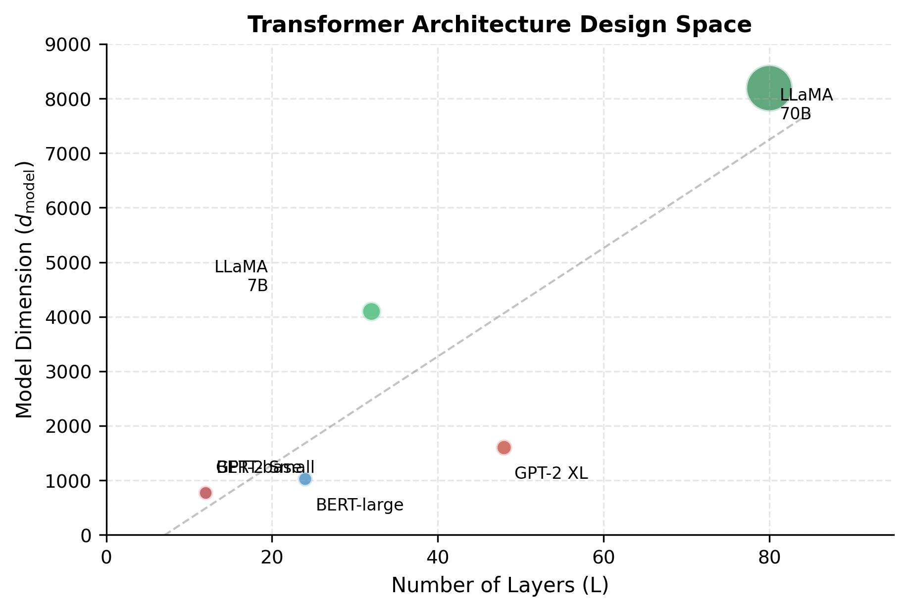
This scatter plot reveals that successful architectures don't maximize just one dimension. Instead, they follow a roughly linear relationship between depth and width, scaling both together. The diagonal trend suggests an empirical consensus about optimal proportions.

Given a fixed parameter budget, should you build a deep, narrow model or a shallow, wide one? This fundamental question shapes every transformer design decision. Think of it like allocating floors and square footage in a building: you can build a tall skyscraper with modest floor plans, or a sprawling low-rise complex. Both might have similar total space, but they serve different purposes.

Depth, the number of transformer layers, determines how many sequential processing stages information passes through. Each layer can refine, combine, and abstract the representations from the previous layer. This sequential refinement is crucial for tasks requiring multi-step reasoning: understanding that "the trophy wouldn't fit in the suitcase because it was too big" requires first parsing the sentence, then resolving "it" to either trophy or suitcase, then applying physical reasoning. Deeper models have more opportunities for such compositional processing.

Width, primarily governed by $d_{\text{model}}$, determines how rich each representation can be. A wider model can encode more nuanced distinctions at each layer: more semantic dimensions, finer-grained syntactic features, more factual associations. Think of width as the vocabulary of concepts available at each processing stage.

Research has revealed important patterns in how these two dimensions contribute to capability. Deeper models tend to develop hierarchical representations, with early layers capturing surface patterns (word shapes, common phrases) and later layers capturing abstractions (sentiment, intent, reasoning chains). Wider models have more capacity per layer but may not develop the same hierarchical structure, instead learning richer but flatter representations.

Understanding this trade-off requires knowing how each dimension affects parameter count. Let's derive the relationship from first principles. For a simplified transformer (ignoring biases and layer norms for clarity), the main parameter contributors are:

• Embedding layer: $V \times d_{\text{model}}$ parameters
• Attention (per layer): $4 \times d_{\text{model}}^2$ parameters (Q, K, V, and output projections)
• FFN (per layer): $2 \times d_{\text{model}} \times d_{\text{ff}}$ parameters (two weight matrices)
• Output projection: Often tied to embeddings, so 0 additional parameters

Summing these components gives us the total parameter count for a transformer model:

where:

• $V$: vocabulary size (number of unique tokens)
• $d_{\text{model}}$: model dimension (hidden size)
• $L$: number of transformer layers
• $d_{\text{ff}}$: feed-forward hidden dimension
• $4 \cdot d_{\text{model}}^2$: attention parameters per layer (four projection matrices: Q, K, V, O)
• $2 \cdot d_{\text{model}} \cdot d_{\text{ff}}$: FFN parameters per layer (two weight matrices: up-projection and down-projection)

For large models, the embedding term $V \cdot d_{\text{model}}$ becomes negligible compared to the layer terms. With the standard expansion ratio $d_{\text{ff}} = 4 \times d_{\text{model}}$, we can simplify by substituting this relationship into the per-layer FFN term:

Adding the attention term gives us the simplified total:

This formula reveals a key insight about scaling behavior: parameters scale linearly with depth $L$ but quadratically with width $d_{\text{model}}$. Doubling the depth doubles the parameters; doubling the width quadruples them.

Although both configurations have similar total parameters, their characteristics differ significantly. The deep model processes information through 48 stages of refinement. The wide model has only 12 stages but can represent much richer information at each stage. Research by Tay et al. (2021) and others suggests that for language modeling, depth tends to be more important, but the optimal ratio depends on the specific task and compute constraints.

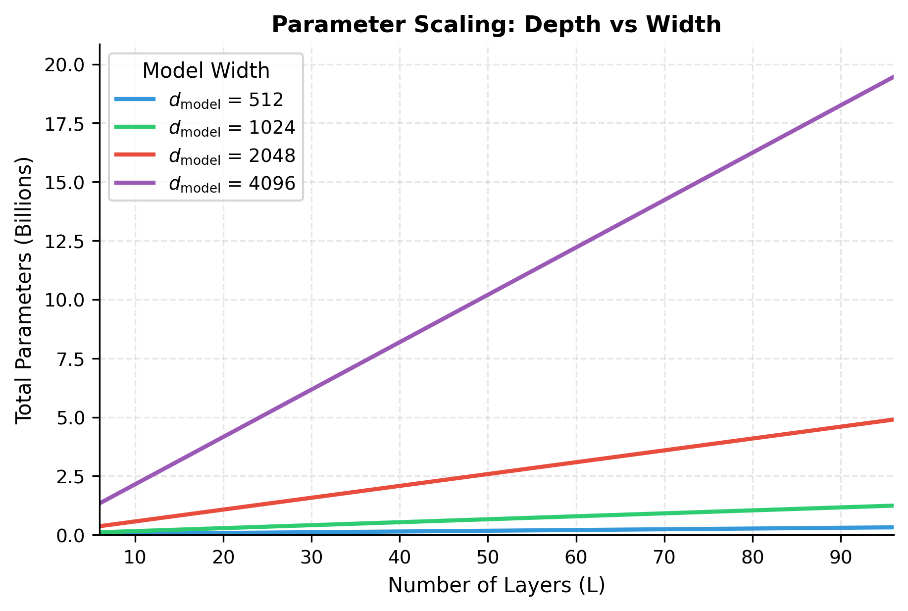
The visualization shows why width is so costly: moving from $d_{\text{model}} = 2048$ to $d_{\text{model}} = 4096$ quadruples the parameters at every depth level. In contrast, adding layers adds parameters linearly. This explains why many successful architectures (like GPT-3 and LLaMA) achieve large parameter counts primarily through depth, keeping width moderate.

The depth-width trade-off isn't just theoretical. Large-scale empirical studies have quantified how each dimension affects model capability as a function of compute budget. Scaling laws research, notably by Hoffmann et al. (2022) in the Chinchilla paper, provides rigorous guidance on optimal model shapes.

The Chinchilla findings were striking: most large language models were undertrained. Given a fixed compute budget, models achieved better performance with fewer parameters and more training data than the prevailing GPT-3 style of maximizing model size. But within the model size constraint, how should parameters be distributed between depth and width?

Studies have found that:

• Depth should scale roughly as the square root of the parameter count
• Width should scale similarly to depth
• The ratio of depth to width (in terms of $d_{\text{model}}$) tends to stay fairly constant across scales

Modern frontier models follow these principles. LLaMA-7B has 32 layers and $d_{\text{model}} = 4096$, giving a ratio of about 128. LLaMA-70B has 80 layers and $d_{\text{model}} = 8192$, maintaining a similar ratio of about 100. This consistency suggests that the field has converged on roughly optimal proportions.

Multi-head attention works by splitting the model dimension into parallel "heads," each computing its own attention pattern independently. One head might attend to syntactic relationships (subject-verb agreement), another to semantic similarity (synonyms and related concepts), and yet another to positional patterns (nearby words). This parallel structure allows the model to capture multiple types of relationships simultaneously.

But how many heads should you use? The answer involves a fundamental trade-off. More heads mean more parallel attention patterns, enabling the model to track more distinct relationships. Fewer heads mean each head has more dimensions to work with, enabling richer attention computations per head. Since the model dimension must be divided among heads, you can't maximize both simultaneously.

The key constraint is that $d_{\text{model}}$ must be evenly divisible by $n_{\text{heads}}$. This divisibility requirement determines the per-head dimension:

where:

• $d_{\text{head}}$: the dimension of queries, keys, and values within each attention head
• $d_{\text{model}}$: the model's hidden dimension
• $n_{\text{heads}}$: the number of parallel attention heads

More heads mean smaller per-head dimensions. With $d_{\text{model}} = 768$ and 12 heads, each head has 64 dimensions. With 24 heads, each would have only 32 dimensions. The trade-off is between having many specialized heads versus having fewer but more expressive heads.

The number of valid configurations varies with model dimension. Highly composite numbers like 768 (which factors as $2^8 \times 3 = 256 \times 3$) offer many choices, while prime-heavy dimensions constrain options. Model designers often choose dimensions specifically for their factorization properties.

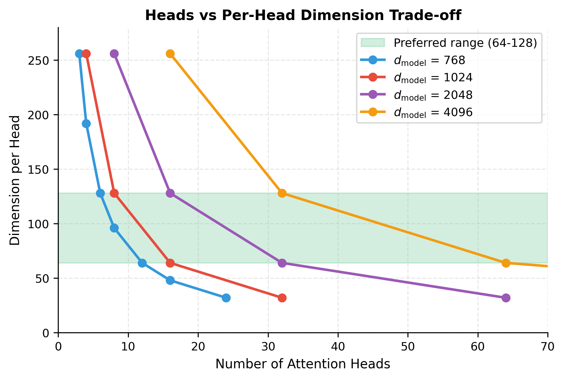
The curves illustrate the fundamental constraint: for any model dimension, increasing heads necessarily decreases per-head dimension. The shaded zone shows where most successful architectures operate. Too few heads (right side of curves, high per-head dimension) means limited parallel attention patterns. Too many heads (left side, low per-head dimension) means each head lacks capacity for meaningful computation.

During autoregressive generation, transformers face a memory bottleneck: they must store the key and value vectors for every previous token in the sequence. This "KV cache" grows linearly with sequence length and can dominate GPU memory for long contexts. With 32 heads and 128-dimensional vectors, a 4096-token context requires storing over 33 million floating-point values per layer, just for the cache.

Modern architectures address this through an elegant asymmetry: reduce the number of key-value heads while keeping query heads high. The insight is that queries need fine-grained distinctions (each position asks different questions), but keys and values can be shared across groups of queries without significant quality loss. This design, called grouped-query attention (GQA), dramatically reduces cache size while preserving most of the model's expressiveness.

To understand the parameter and memory implications, let's examine how projections work in standard multi-head attention. Each head has its own Q, K, and V projections, with parameter counts computed as the product of the number of heads, the per-head dimension, and the model dimension:

• Q projections: $n_{\text{heads}} \times d_{\text{head}} \times d_{\text{model}}$ parameters
• K projections: $n_{\text{heads}} \times d_{\text{head}} \times d_{\text{model}}$ parameters
• V projections: $n_{\text{heads}} \times d_{\text{head}} \times d_{\text{model}}$ parameters
• Output projection: $n_{\text{heads}} \times d_{\text{head}} \times d_{\text{model}}$ parameters

where $n_{\text{heads}}$ is the number of attention heads, $d_{\text{head}}$ is the dimension per head, and $d_{\text{model}}$ is the model dimension. Since $n_{\text{heads}} \times d_{\text{head}} = d_{\text{model}}$, each projection contributes $d_{\text{model}}^2$ parameters.

In grouped-query attention (GQA) with $n_{\text{kv\_heads}}$ key-value heads, the K and V projections are shared across groups of query heads:

• Q projections: unchanged ($n_{\text{heads}} \times d_{\text{head}} \times d_{\text{model}}$)
• K projections: reduced ($n_{\text{kv\_heads}} \times d_{\text{head}} \times d_{\text{model}}$)
• V projections: reduced ($n_{\text{kv\_heads}} \times d_{\text{head}} \times d_{\text{model}}$)
• Output projection: unchanged

Each group of $n_{\text{heads}} / n_{\text{kv\_heads}}$ query heads shares the same K and V projections, reducing parameters while maintaining the full expressiveness of query computations.

The parameter savings from GQA are modest (the reduction is only in K and V projections), but the real benefit is during inference. The KV cache, which stores key and value vectors for all previous tokens during autoregressive generation, shrinks proportionally with $n_{\text{kv\_heads}}$. For long sequences, this can be the difference between fitting a model in GPU memory or not.

LLaMA-2 70B uses GQA with 8 KV heads and 64 query heads, reducing KV cache memory by 8x compared to standard MHA while maintaining quality. This design choice enables longer context windows with the same hardware.

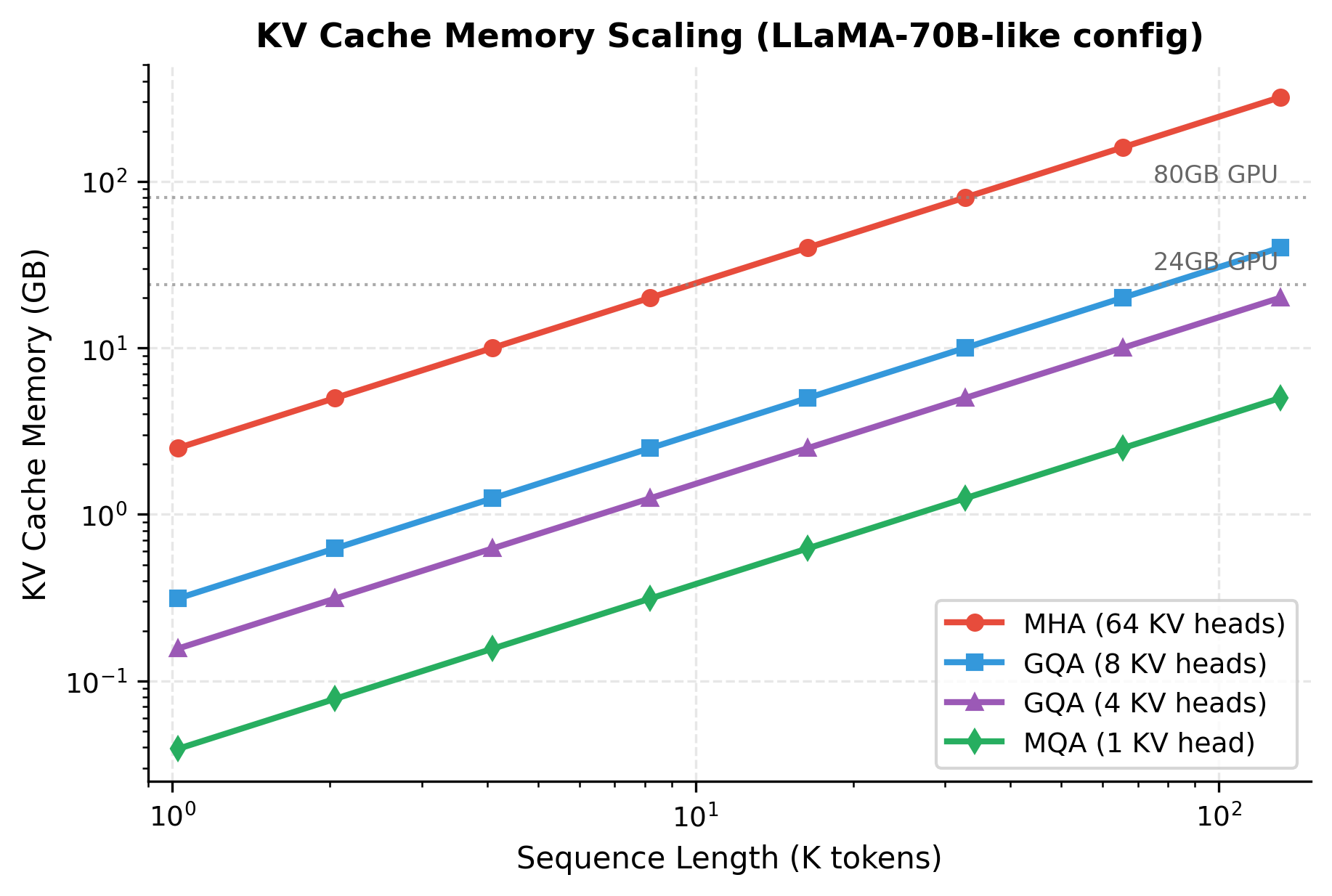
The logarithmic scales reveal the dramatic impact of GQA. At 128K tokens, standard MHA would require over 1TB of KV cache memory (per layer, summed across all layers), while GQA with 8 heads needs only about 130GB. This difference is why long-context models universally adopt GQA or MQA.

While attention layers decide which tokens to combine, the feed-forward network (FFN) performs the actual transformation of each token's representation. This division of labor has a surprising consequence: the FFN contains far more parameters than attention, making it the dominant factor in model size.

Understanding why requires examining what each component does. Attention computes weighted averages of value vectors, a fundamentally linear operation (the only nonlinearity is softmax for computing weights). The FFN, by contrast, applies a nonlinear transformation that can reshape the representation space, activate or suppress features, and encode factual associations. Research has shown that specific FFN neurons activate for particular concepts: "Eiffel Tower," "Python programming," or "past tense verbs." The FFN is where the model stores much of its learned knowledge.

This knowledge-storage role explains why FFNs need substantial capacity. The original transformer paper established the convention $d_{\text{ff}} = 4 \times d_{\text{model}}$, providing the FFN with four times more hidden dimensions than the model's representation size. This 4x expansion gives each layer a wide intermediate space for computation before projecting back to $d_{\text{model}}$ dimensions.

Let's derive exactly how this expansion affects parameter counts and understand why FFNs dominate model size.

For a standard two-layer FFN, the computation applies an up-projection, activation, and down-projection:

where:

• $\mathbf{x} \in \mathbb{R}^{d_{\text{model}}}$: the input vector (one token's representation)
• $\mathbf{W}_1 \in \mathbb{R}^{d_{\text{model}} \times d_{\text{ff}}}$: the up-projection weight matrix
• $\mathbf{W}_2 \in \mathbb{R}^{d_{\text{ff}} \times d_{\text{model}}}$: the down-projection weight matrix
• $\mathbf{b}_1 \in \mathbb{R}^{d_{\text{ff}}}$, $\mathbf{b}_2 \in \mathbb{R}^{d_{\text{model}}}$: bias vectors
• $\text{GELU}(\cdot)$: the Gaussian Error Linear Unit activation function

The total parameter count includes both weight matrices and bias vectors:

The first term accounts for the two weight matrices (each with $d_{\text{model}} \times d_{\text{ff}}$ parameters), while the remaining terms count the bias vectors. With the standard expansion ratio $d_{\text{ff}} = 4 \times d_{\text{model}}$ and ignoring the relatively small bias terms:

Compare this to attention parameters for standard multi-head attention (MHA), which has four projection matrices (Q, K, V, and output), each of size $d_{\text{model}} \times d_{\text{model}}$:

The FFN has twice as many parameters as attention. This 2:1 ratio is consistent across most transformer architectures and explains why FFN optimization is so important for efficiency.

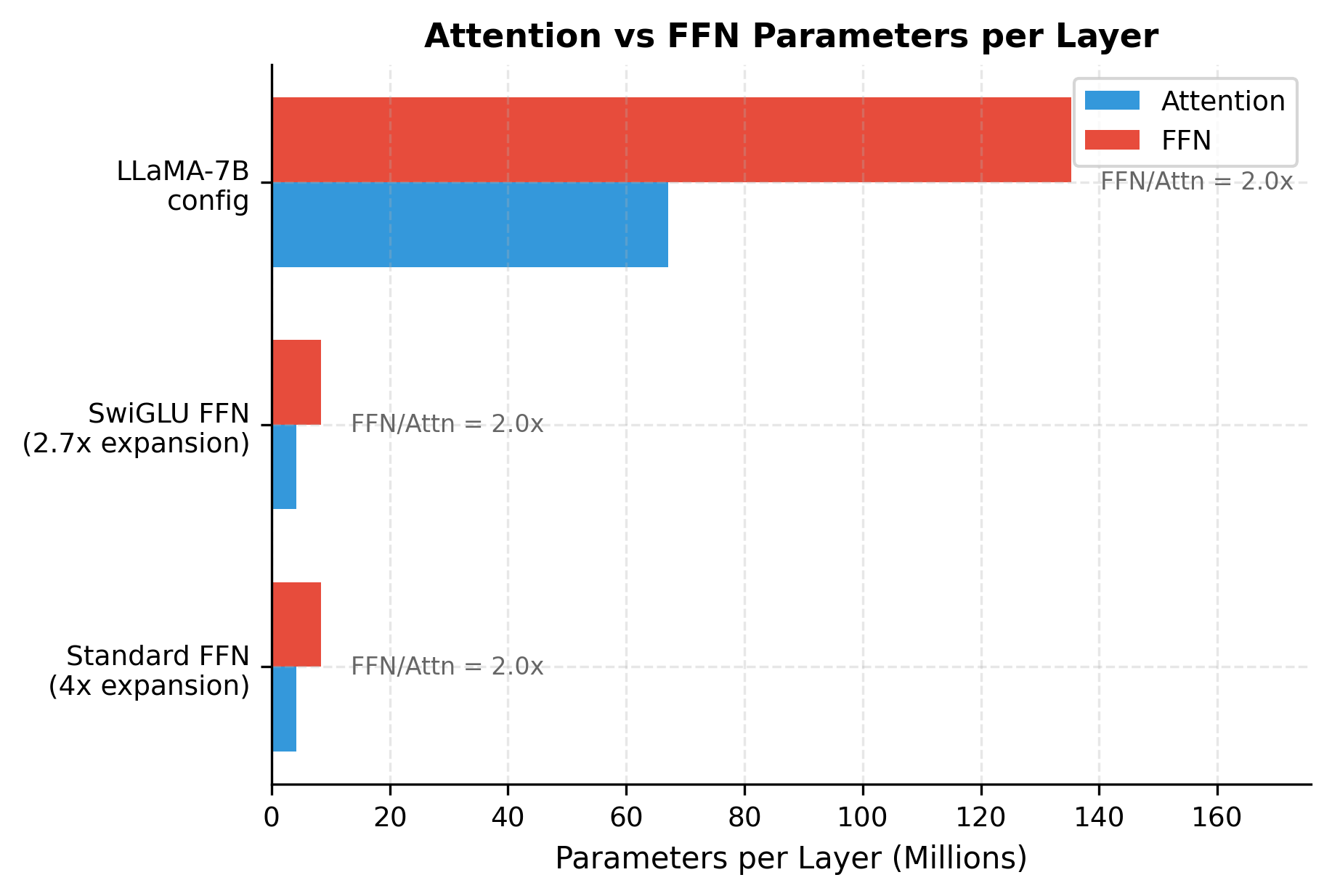
The visualization confirms that regardless of architecture choice, FFN parameters dominate. Even with SwiGLU's reduced expansion ratio, the FFN still accounts for roughly twice the parameters of attention. This consistent 2:1 ratio has important implications for optimization techniques like mixture-of-experts, which specifically target FFN layers.

The standard FFN applies a simple pattern: project up, apply nonlinearity, project down. But research has shown that adding a gating mechanism can improve performance significantly. The gating idea comes from LSTMs and GRUs: instead of passing all information through uniformly, learn which dimensions to emphasize and which to suppress.

SwiGLU (SiLU-Gated Linear Unit) implements this by computing two parallel projections of the input. One projection becomes the "content" that might pass through. The other projection, after applying the SiLU activation, becomes the "gate" that controls how much of each dimension actually passes. The element-wise product of content and gate creates a selective filtering effect.

This gating mechanism requires three weight matrices instead of two:

where:

• $\mathbf{x} \in \mathbb{R}^{d_{\text{model}}}$: the input vector
• $\mathbf{W}_{\text{gate}} \in \mathbb{R}^{d_{\text{model}} \times d_{\text{ff}}}$: the gate projection matrix
• $\mathbf{W}_{\text{up}} \in \mathbb{R}^{d_{\text{model}} \times d_{\text{ff}}}$: the up-projection matrix
• $\mathbf{W}_{\text{down}} \in \mathbb{R}^{d_{\text{ff}} \times d_{\text{model}}}$: the down-projection matrix
• $\text{SiLU}(\cdot)$: the Sigmoid Linear Unit activation (also called Swish)
• $\odot$: element-wise multiplication

With three matrices each containing $d_{\text{model}} \times d_{\text{ff}}$ parameters, the total count is:

To maintain the same parameter count as a standard FFN with 4x expansion, we can solve for the required SwiGLU expansion ratio. Setting the SwiGLU parameter count equal to the standard FFN count:

Dividing both sides by $3 \times d_{\text{model}}$ gives the required FFN dimension:

In practice, $d_{\text{ff}}$ is often rounded to a multiple of 256 for efficient GPU computation. LLaMA uses $d_{\text{ff}} = 2.6875 \times d_{\text{model}}$ (specifically 11008 for $d_{\text{model}} = 4096$), which is close to the theoretical value of $\frac{8}{3} \times 4096 = 10923$.

The three configurations have nearly identical parameter counts, demonstrating that SwiGLU's third matrix is compensated by the smaller expansion ratio. This equivalence is intentional: it allows fair comparisons between architectures and predictable parameter budgets.

We've now examined each component of a transformer: embeddings that map tokens to vectors, attention mechanisms that mix information across positions, and feed-forward networks that transform each position independently. To design architectures or understand published models, we need to combine these pieces into a complete parameter count.

This matters for several practical reasons:

1. Hardware planning: GPU memory limits how many parameters you can train. A 70B parameter model in FP16 requires 140GB just for weights, before accounting for optimizer states, activations, or gradients.

2. Cost estimation: Training compute scales with parameter count. Knowing your model's size helps estimate training time and cost.

3. Architecture verification: When implementing published models, parameter counting helps verify your implementation matches the original.

4. Design iteration: When exploring architectures, quick parameter estimates help evaluate trade-offs without running experiments.

Let's build a comprehensive parameter calculator that breaks down contributions from each component.

Let's verify our calculator against known model sizes:

Our calculations align with published model sizes. Note how the embedding fraction decreases dramatically as models scale: for GPT-2 Small, embeddings represent a significant fraction of parameters, but for LLaMA-70B, the transformer layers dominate overwhelmingly. This is why larger models are more parameter-efficient: the fixed embedding cost amortizes over more layer parameters.

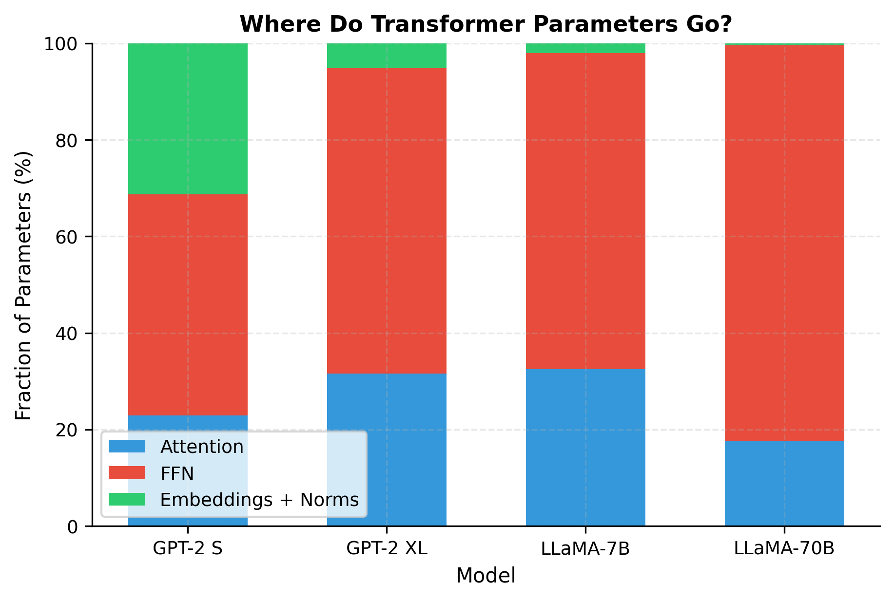
The visualization confirms what the numbers suggested: as models grow, FFN parameters increasingly dominate. The FFN is the workhorse of parameter storage, containing roughly twice the parameters of attention in each layer. This explains why techniques like mixture-of-experts (MoE), which primarily target FFN layers, can dramatically increase effective capacity.

We've now covered the individual hyperparameters: depth, width, heads, FFN dimensions, and their variants. But knowing what each parameter does is different from knowing how to choose values. Architecture design is both an art and a science, combining theoretical understanding with empirical intuition and practical constraints.

The good news is that the field has converged on patterns that work. Successful open models like LLaMA, Mistral, and Qwen share similar proportions, and these patterns provide reliable starting points for new designs. The following principles distill this collective wisdom into actionable guidance.

Rather than searching the vast space of possible architectures, begin with ratios that have proven successful across many models and tasks:

• $d_{\text{ff}} = 4 \times d_{\text{model}}$ for standard FFN, or $\approx 2.7 \times d_{\text{model}}$ for SwiGLU
• $d_{\text{head}} \in [64, 128]$, which determines $n_{\text{heads}} = d_{\text{model}} / d_{\text{head}}$
• Depth/width ratio: $L \approx d_{\text{model}} / 100$ to $d_{\text{model}} / 50$ (very rough guideline)

These suggestions provide reasonable starting points, but optimal architectures depend on hardware constraints, training budget, and intended use case. The suggestions follow the pattern of successful open models, scaling both depth and width together while maintaining consistent per-head dimensions.

The best architecture on paper can be the worst in practice if it doesn't align with hardware constraints. Modern GPUs have specific requirements for efficient matrix operations, and dimensions that seem arbitrary (like 11008 instead of 11000) often reflect careful optimization for these constraints.

Efficient computation requires dimensions that align with hardware characteristics. Key considerations include:

• Tensor core alignment: NVIDIA tensor cores work most efficiently with dimensions that are multiples of 8 (for FP16) or 16 (for INT8). Multiples of 64 or 128 are even better.
• Memory alignment: Dimensions that are powers of 2 or multiples of 256 often achieve better memory bandwidth utilization.
• Parallelism: The number of heads should divide evenly across GPUs in tensor-parallel setups. For 8-GPU training, 32 or 64 heads work well.

LLaMA's configuration is carefully chosen for hardware efficiency. The model dimension and head count align perfectly, and the FFN dimension is chosen to balance parameter equivalence with computational efficiency (11008 is close to the theoretical 10923 but rounds to a more efficient value).

Architecture design doesn't happen in isolation. The optimal model shape depends on how you'll train it, how long your sequences are, and where you'll deploy it. A model optimized for training efficiency might be suboptimal for inference, and vice versa. Consider the full pipeline from training to deployment.

Key interactions to consider:

• Sequence length: Longer sequences increase memory for attention (quadratic in sequence length) and KV cache. GQA becomes more valuable for long-context models.
• Batch size: Larger batches favor wider models that can better utilize parallel computation.
• Training tokens: Scaling laws suggest parameter count and training data should scale together. A 7B model typically needs 1-2 trillion tokens for optimal performance.
• Inference hardware: If deploying to specific hardware, optimize dimensions for that target rather than for training efficiency.

Transformer architecture hyperparameters determine model capacity, computational requirements, and ultimately performance. The key takeaways from this chapter are:

• Six core hyperparameters define a transformer: vocabulary size ($V$), layers ($L$), model dimension ($d_{\text{model}}$), attention heads ($n_{\text{heads}}$), head dimension ($d_{\text{head}}$), and FFN dimension ($d_{\text{ff}}$). Everything else derives from these choices.

• Depth scales linearly, width quadratically. Doubling the number of layers doubles parameters; doubling the model dimension quadruples them. This makes depth a more parameter-efficient way to add capacity, but both contribute to model expressiveness in different ways.

• Head dimensions cluster around 64-128. This empirical sweet spot balances per-head capacity with the benefits of multiple parallel attention mechanisms. The number of heads is then determined by $n_{\text{heads}} = d_{\text{model}} / d_{\text{head}}$.

• FFN expansion follows predictable ratios. Standard FFNs use $d_{\text{ff}} = 4 \times d_{\text{model}}$, while SwiGLU-based FFNs use approximately $2.7 \times d_{\text{model}}$ to maintain equivalent parameter counts.

• Grouped-query attention trades parameters for memory. GQA reduces KV cache size during inference by sharing key-value projections across multiple query heads, enabling longer context windows without proportional memory increases.

• FFN dominates parameter counts. At larger scales, feed-forward networks contain the majority of parameters, making them the primary target for efficiency innovations like mixture-of-experts.

• Hardware alignment matters. Dimensions should be multiples of 8, 64, or 128 for efficient tensor core utilization. The number of heads should divide evenly across GPUs for tensor parallelism.

When designing a new architecture, start with proven configurations from similar-scale models, ensure hardware-friendly dimensions, and adjust based on your specific constraints and empirical results. The art of architecture design lies in balancing these considerations while respecting the fundamental trade-offs between capacity, compute, and memory.

When designing or analyzing transformer architectures, the following parameters have the most significant impact:

• $L$ (number of layers): Controls model depth and hierarchical abstraction capability. Start with 12-24 layers for smaller models (< 1B parameters) and scale to 32-80+ for larger models. Deeper models generally improve reasoning and multi-step tasks but require more careful initialization and training stability measures.

• $d_{\text{model}}$ (model dimension): The primary driver of per-layer capacity. Should be a multiple of 128 for optimal hardware utilization. Common values range from 768 (small models) to 8192 (frontier models). Quadratic impact on parameters means width is expensive.

• $n_{\text{heads}}$ (attention heads): Determines how many parallel attention patterns the model can learn. Set based on desired $d_{\text{head}}$: for $d_{\text{head}} = 64$, use $n_{\text{heads}} = d_{\text{model}} / 64$. More heads allow finer-grained attention but increase overhead.

• $d_{\text{head}}$ (head dimension): Target 64-128 for most applications. Smaller values allow more heads but reduce per-head expressiveness. Larger values (256+) rarely improve performance and reduce head count.

• $d_{\text{ff}}$ (FFN dimension): Set to $4 \times d_{\text{model}}$ for standard FFN or approximately $2.7 \times d_{\text{model}}$ for SwiGLU. Round to multiples of 256 for efficient GPU computation. This parameter dominates total parameter count.

• $n_{\text{kv\_heads}}$ (GQA heads): For inference-optimized models, reduce KV heads to 8-16 regardless of query head count. Reduces KV cache memory proportionally with minimal quality loss. Essential for long-context models.

• $V$ (vocabulary size): Typically 32K-100K tokens. Larger vocabularies improve compression but increase embedding memory. Choose based on target languages and tokenization strategy.

Ready to test your understanding? Take this quick quiz to reinforce what you've learned about transformer architecture hyperparameters.