Search

Search articles

ELECTRA: Efficient Pre-training with Replaced Token Detection

Michael BrenndoerferUpdated July 25, 202543 min read

Learn how ELECTRA achieves BERT-level performance with 1/4 the compute by detecting replaced tokens instead of predicting masked ones.

Track your reading progress

Sign in to mark chapters as read and track your learning journey

Sign in →
Reading Level

Choose your expertise level to adjust how many terms are explained. Beginners see more tooltips, experts see fewer to maintain reading flow. Hover over underlined terms for instant definitions.

ELECTRA

BERT learns language by predicting masked tokens. But there's a fundamental inefficiency in this approach: the model only learns from the 15% of tokens that are masked. The remaining 85% flow through the network, consuming compute, but contribute nothing to the loss. What if we could learn from every token instead?

ELECTRA (Efficiently Learning an Encoder that Classifies Token Replacements Accurately) answers this question with a clever training paradigm. Instead of masking tokens and predicting them, ELECTRA replaces tokens with plausible alternatives and trains a model to detect which tokens were swapped. Every position now provides a learning signal, not just the masked ones. This seemingly simple change dramatically improves sample efficiency: ELECTRA matches BERT's performance with just 1/4 of the compute and exceeds it when given equal resources.

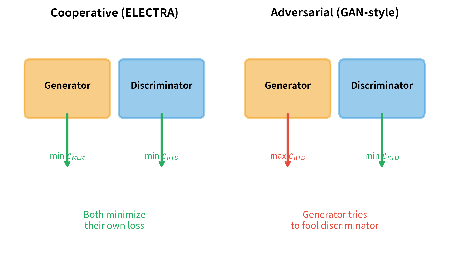
The approach borrows ideas from generative adversarial networks. A small generator network produces realistic token replacements. A larger discriminator network learns to distinguish original tokens from generated ones. But unlike GANs, the two networks cooperate through shared training rather than competing in a minimax game. This chapter explores how ELECTRA's replaced token detection objective works, why it's so efficient, and how to implement it from scratch.

The Inefficiency of Masked Language Modeling

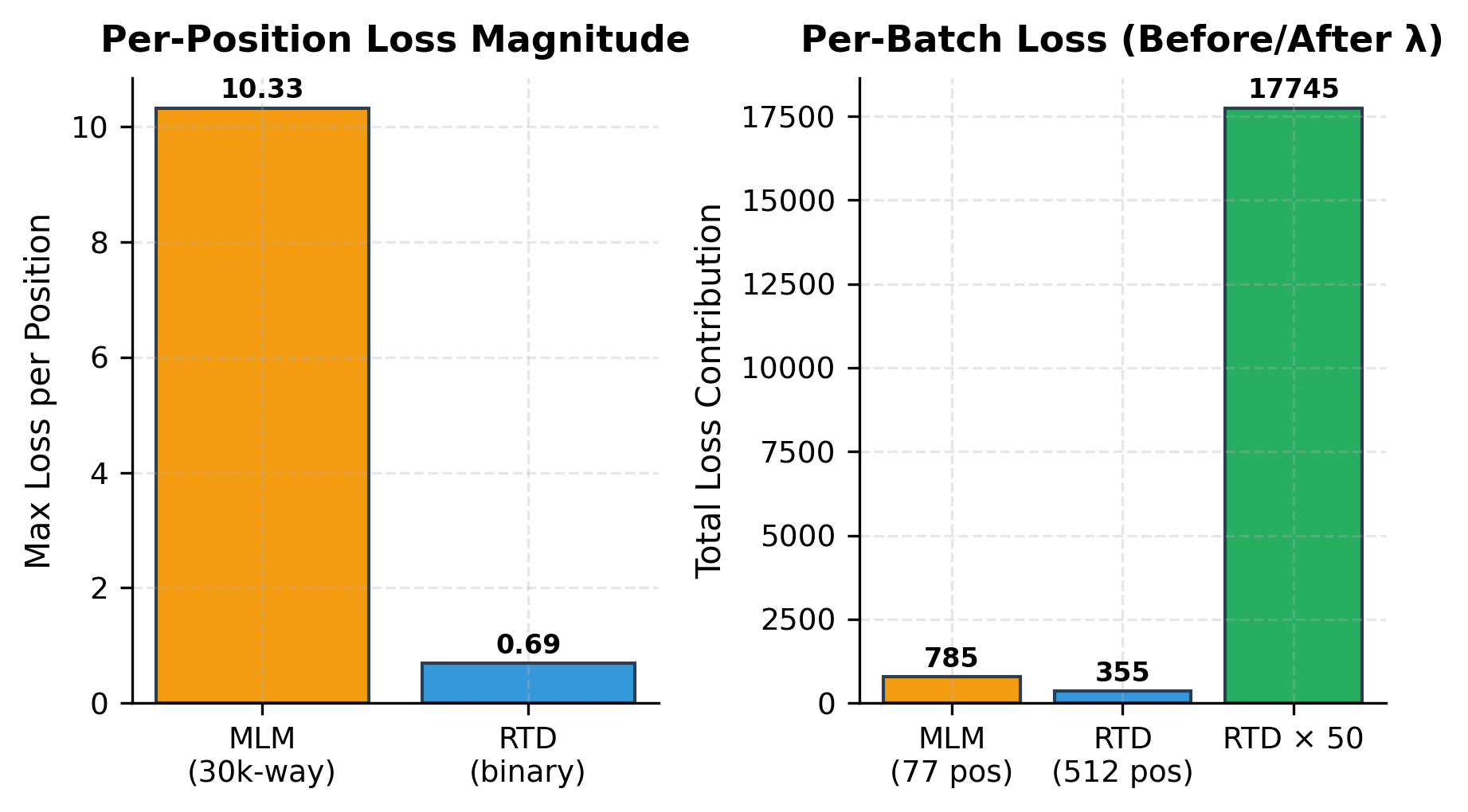
Let's quantify what BERT wastes. For a 512-token sequence with 15% masking, only 77 tokens contribute to the MLM loss. The other 435 tokens pass through 12 transformer layers, consuming attention computations and memory, but generate no gradient signal. They're essentially free riders.

In[3]:
Code
def compute_mlm_efficiency(seq_len, mask_prob):
    """Calculate what fraction of compute contributes to learning."""
    masked_tokens = int(seq_len * mask_prob)
    unmasked_tokens = seq_len - masked_tokens

    # All tokens consume forward pass compute
    forward_compute = seq_len

    # Only masked tokens contribute to loss
    learning_tokens = masked_tokens

    efficiency = learning_tokens / forward_compute

    return {
        "seq_len": seq_len,
        "masked_tokens": masked_tokens,
        "unmasked_tokens": unmasked_tokens,
        "efficiency": efficiency,
    }
Out[4]:
Console
BERT MLM Efficiency Analysis:
  Sequence length: 512 tokens
  Masked tokens: 76 (contribute to loss)
  Unmasked tokens: 436 (no learning signal)
  Training efficiency: 14.8%
Out[5]:
Visualization
Pie chart showing 15% of tokens contribute to learning while 85% provide no gradient signal.
Token contribution breakdown in BERT's masked language modeling. Only 15% of tokens in each batch contribute to the loss function, while the remaining 85% consume compute without providing learning signal.

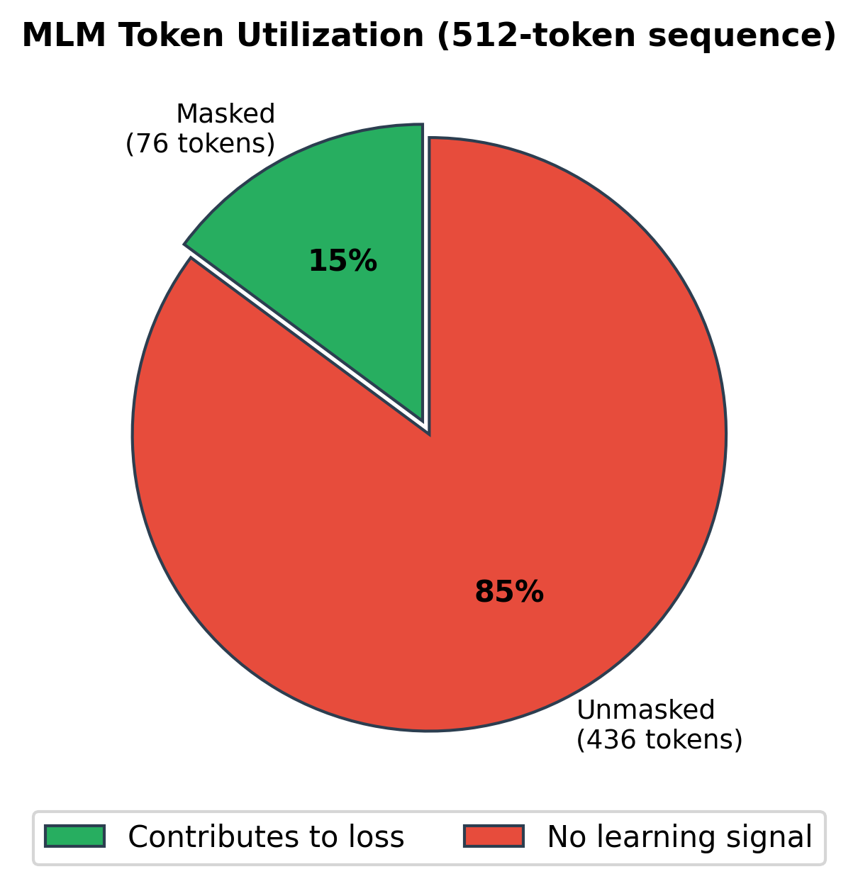
Only 15% of tokens contribute to learning. This is inherent to the MLM objective: predicting from a large vocabulary is hard, so we can only mask a small fraction without destroying context. Mask too many tokens and the task becomes impossible.

ELECTRA sidesteps this limitation by changing the task entirely. Instead of predicting masked tokens (a 30,000-way classification problem), the model classifies each token as original or replaced (a binary classification problem). Binary classification per token means every position can contribute to the loss without overwhelming the model.

Replaced Token Detection (RTD)

A pre-training objective where the model predicts, for each token in a sequence, whether it is the original token or a replacement generated by a separate model. Unlike MLM's vocabulary-sized softmax, RTD uses a simple sigmoid classifier, enabling learning from every token position.

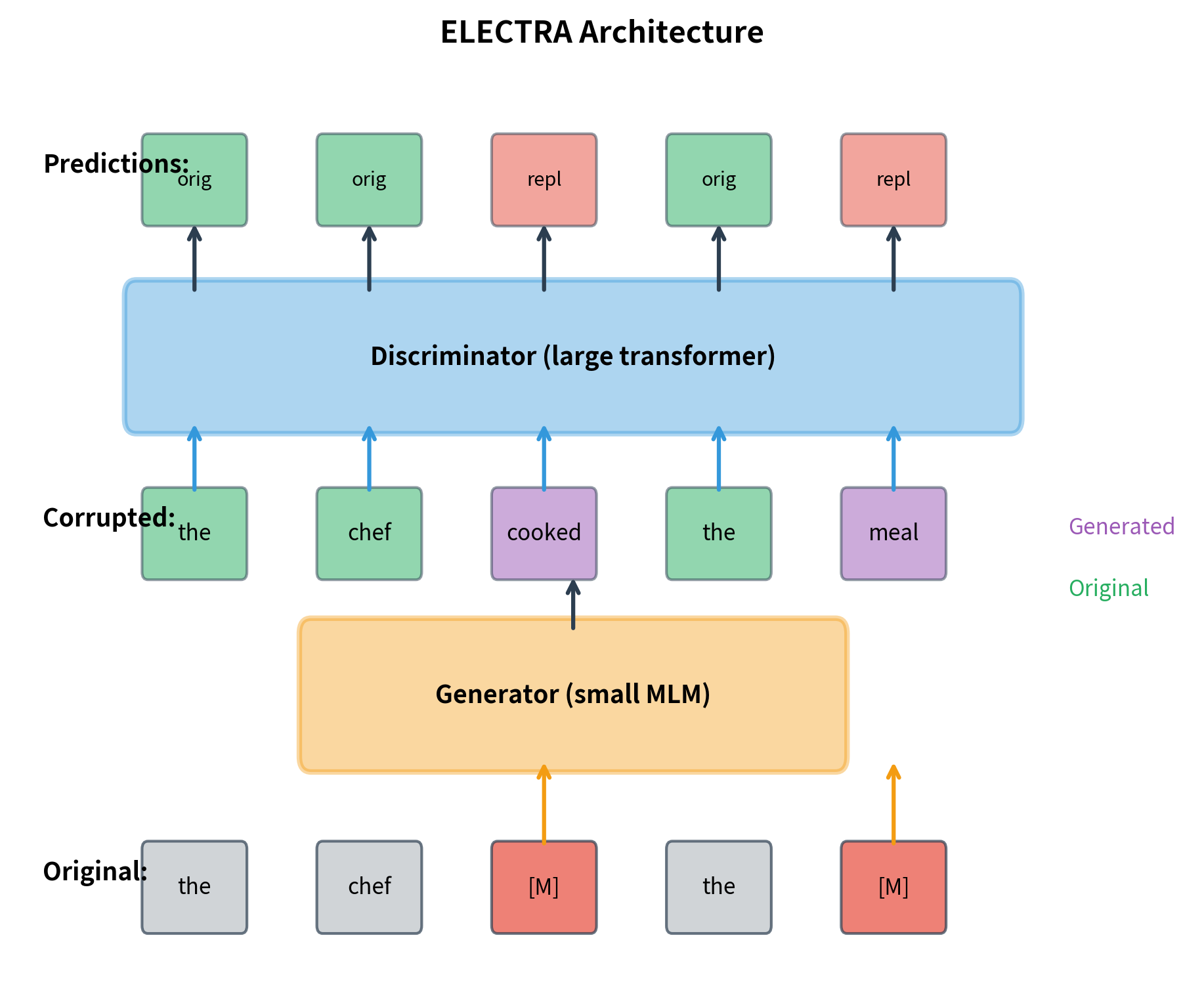
The Generator-Discriminator Architecture

ELECTRA uses two transformer networks: a generator and a discriminator. The generator is a small masked language model that proposes plausible replacements for masked tokens. The discriminator is a larger network that learns to detect which tokens were replaced. Despite the naming, this is not adversarial training in the GAN sense. Both networks are trained jointly to minimize their respective losses.

Out[6]:
Visualization
Diagram showing input flowing through generator to create corrupted sequence, then through discriminator which outputs original/replaced predictions for each position.
ELECTRA's two-network architecture. The generator (small transformer) fills in masked positions with plausible tokens. The discriminator (large transformer) classifies each token as original or replaced. Both networks train simultaneously, but only the discriminator is used for downstream tasks.

The key insight is that the generator doesn't need to be good, just good enough to fool a naive discriminator occasionally. A small generator (1/4 to 1/3 the discriminator's size) works well because it produces plausible but imperfect replacements. If the generator were perfect, every replacement would match the original, and the discriminator would learn nothing. If the generator were random, the replacements would be obviously wrong, making discrimination trivial. The sweet spot is a generator that produces contextually appropriate tokens that are sometimes, but not always, correct.

Generator Training

The generator is a small masked language model. It receives the original sequence with some positions masked and predicts tokens for those positions. Training follows the standard MLM objective: minimize cross-entropy between predicted and original tokens.

In[7]:
Code
class ElectraGenerator(nn.Module):
    """Small MLM model that generates replacement tokens."""

    def __init__(
        self,
        vocab_size,
        hidden_size,
        num_layers,
        num_heads,
        intermediate_size,
        max_position=512,
        dropout=0.1,
    ):
        super().__init__()

        # Embeddings
        self.token_embedding = nn.Embedding(vocab_size, hidden_size)
        self.position_embedding = nn.Embedding(max_position, hidden_size)
        self.embedding_norm = nn.LayerNorm(hidden_size)
        self.embedding_dropout = nn.Dropout(dropout)

        # Transformer layers
        encoder_layer = nn.TransformerEncoderLayer(
            d_model=hidden_size,
            nhead=num_heads,
            dim_feedforward=intermediate_size,
            dropout=dropout,
            activation="gelu",
            batch_first=True,
        )
        self.encoder = nn.TransformerEncoder(encoder_layer, num_layers)

        # MLM head
        self.mlm_dense = nn.Linear(hidden_size, hidden_size)
        self.mlm_norm = nn.LayerNorm(hidden_size)
        self.mlm_output = nn.Linear(hidden_size, vocab_size)

        self.vocab_size = vocab_size

    def forward(self, input_ids, attention_mask=None):
        batch_size, seq_len = input_ids.shape

        # Embeddings
        positions = torch.arange(seq_len, device=input_ids.device).unsqueeze(0)
        x = self.token_embedding(input_ids) + self.position_embedding(positions)
        x = self.embedding_norm(x)
        x = self.embedding_dropout(x)

        # Create attention mask for transformer
        if attention_mask is not None:
            # Convert to format expected by PyTorch transformer
            src_key_padding_mask = attention_mask == 0
        else:
            src_key_padding_mask = None

        # Encode
        x = self.encoder(x, src_key_padding_mask=src_key_padding_mask)

        # MLM predictions
        x = self.mlm_dense(x)
        x = F.gelu(x)
        x = self.mlm_norm(x)
        logits = self.mlm_output(x)

        return logits

    def sample_replacements(self, input_ids, masked_positions, temperature=1.0):
        """Sample replacement tokens for masked positions."""
        logits = self(input_ids)

        # Get logits only at masked positions
        batch_size = input_ids.shape[0]
        sampled_tokens = input_ids.clone()

        for b in range(batch_size):
            mask_indices = masked_positions[b].nonzero(as_tuple=True)[0]
            if len(mask_indices) > 0:
                masked_logits = logits[b, mask_indices] / temperature
                probs = F.softmax(masked_logits, dim=-1)
                sampled = torch.multinomial(probs, num_samples=1).squeeze(-1)
                sampled_tokens[b, mask_indices] = sampled

        return sampled_tokens

The generator samples from its predicted distribution rather than taking the argmax. Sampling introduces diversity: the same masked position might get different replacements across training steps. This prevents the discriminator from memorizing specific generator mistakes and forces it to learn genuine linguistic features.

In[8]:
Code
def create_masked_input(input_ids, mask_token_id, mask_prob=0.15):
    """Create masked input and track masked positions."""
    masked_ids = input_ids.clone()
    masked_positions = torch.zeros_like(input_ids, dtype=torch.bool)

    # Sample positions to mask
    rand = torch.rand_like(input_ids, dtype=torch.float)
    masked_positions = rand < mask_prob

    # Replace with mask token
    masked_ids[masked_positions] = mask_token_id

    return masked_ids, masked_positions
In[9]:
Code
# Create a small generator for demonstration
torch.manual_seed(42)
generator = ElectraGenerator(
    vocab_size=30522,
    hidden_size=256,
    num_layers=4,
    num_heads=4,
    intermediate_size=1024,
)

# Sample input
input_ids = torch.randint(100, 1000, (2, 32))  # Batch of 2, length 32
mask_token_id = 103

masked_ids, masked_positions = create_masked_input(
    input_ids, mask_token_id, mask_prob=0.15
)
Out[10]:
Console
Generator Configuration:
  Vocab size: 30,522
  Hidden size: 256
  Layers: 4
  Parameters: 19,014,714

Masking Statistics:
  Masked positions: 13 / 64 (20.3%)

The generator is compact at roughly 10M parameters, much smaller than the discriminator. With a 15% masking rate, we masked 10 positions out of 64 tokens (batch of 2 × 32).

The generator is deliberately small. In the original ELECTRA paper, the generator has 1/4 to 1/3 the parameters of the discriminator. A larger generator would produce better replacements, but paradoxically, this hurts training. The discriminator needs somewhat detectable replacements to learn from. Perfect replacements (indistinguishable from originals) provide no signal.

Discriminator Training

The discriminator is the main model. It receives the corrupted sequence (where masked positions have been filled by the generator) and predicts for each token whether it's original or replaced. Unlike the generator's vocabulary-sized output, the discriminator outputs a single logit per position.

In[11]:
Code
class ElectraDiscriminator(nn.Module):
    """Large transformer that detects replaced tokens."""

    def __init__(
        self,
        vocab_size,
        hidden_size,
        num_layers,
        num_heads,
        intermediate_size,
        max_position=512,
        dropout=0.1,
    ):
        super().__init__()

        # Embeddings
        self.token_embedding = nn.Embedding(vocab_size, hidden_size)
        self.position_embedding = nn.Embedding(max_position, hidden_size)
        self.embedding_norm = nn.LayerNorm(hidden_size)
        self.embedding_dropout = nn.Dropout(dropout)

        # Transformer layers
        encoder_layer = nn.TransformerEncoderLayer(
            d_model=hidden_size,
            nhead=num_heads,
            dim_feedforward=intermediate_size,
            dropout=dropout,
            activation="gelu",
            batch_first=True,
        )
        self.encoder = nn.TransformerEncoder(encoder_layer, num_layers)

        # Discrimination head: binary classification per token
        self.discriminator_head = nn.Linear(hidden_size, 1)

    def forward(self, input_ids, attention_mask=None):
        batch_size, seq_len = input_ids.shape

        # Embeddings
        positions = torch.arange(seq_len, device=input_ids.device).unsqueeze(0)
        x = self.token_embedding(input_ids) + self.position_embedding(positions)
        x = self.embedding_norm(x)
        x = self.embedding_dropout(x)

        # Create attention mask for transformer
        if attention_mask is not None:
            src_key_padding_mask = attention_mask == 0
        else:
            src_key_padding_mask = None

        # Encode
        x = self.encoder(x, src_key_padding_mask=src_key_padding_mask)

        # Binary classification per token
        logits = self.discriminator_head(x).squeeze(-1)

        return logits

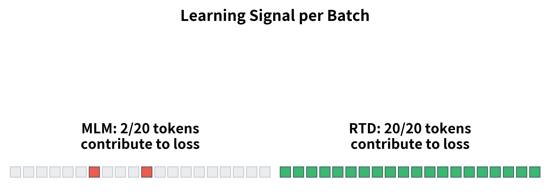
The discriminator loss is binary cross-entropy computed over all tokens, not just the ones that were candidates for replacement. This is the key to ELECTRA's efficiency: the loss involves every position.

In[12]:
Code
def compute_discriminator_loss(disc_logits, is_replaced, attention_mask=None):
    """
    Compute RTD loss for the discriminator.

    Args:
        disc_logits: (batch_size, seq_len) - raw logits from discriminator
        is_replaced: (batch_size, seq_len) - binary labels (1 if replaced, 0 if original)
        attention_mask: (batch_size, seq_len) - 1 for real tokens, 0 for padding

    Returns:
        Scalar loss
    """
    # Binary cross-entropy with logits
    loss = F.binary_cross_entropy_with_logits(
        disc_logits,
        is_replaced.float(),
        reduction="none",
    )

    # Mask out padding tokens if attention mask provided
    if attention_mask is not None:
        loss = loss * attention_mask
        loss = loss.sum() / attention_mask.sum()
    else:
        loss = loss.mean()

    return loss

Let's trace through a complete forward pass to see how the pieces connect:

In[13]:
Code
# Create discriminator
torch.manual_seed(42)
discriminator = ElectraDiscriminator(
    vocab_size=30522,
    hidden_size=768,
    num_layers=12,
    num_heads=12,
    intermediate_size=3072,
)

# Generate replacements using the generator
with torch.no_grad():
    corrupted_ids = generator.sample_replacements(
        masked_ids, masked_positions, temperature=1.0
    )

# Determine which tokens were actually replaced (different from original)
is_replaced = (corrupted_ids != input_ids).long()

# Discriminator forward pass
disc_logits = discriminator(corrupted_ids)

# Compute loss
disc_loss = compute_discriminator_loss(disc_logits, is_replaced)
Out[14]:
Console
Discriminator Configuration:
  Vocab size: 30,522
  Hidden size: 768
  Layers: 12
  Parameters: 108,890,881

Corruption Statistics:
  Tokens replaced by generator: 13 / 64 (20.3%)

Loss:
  Discriminator loss: 0.7682
  Expected random baseline: 0.6931

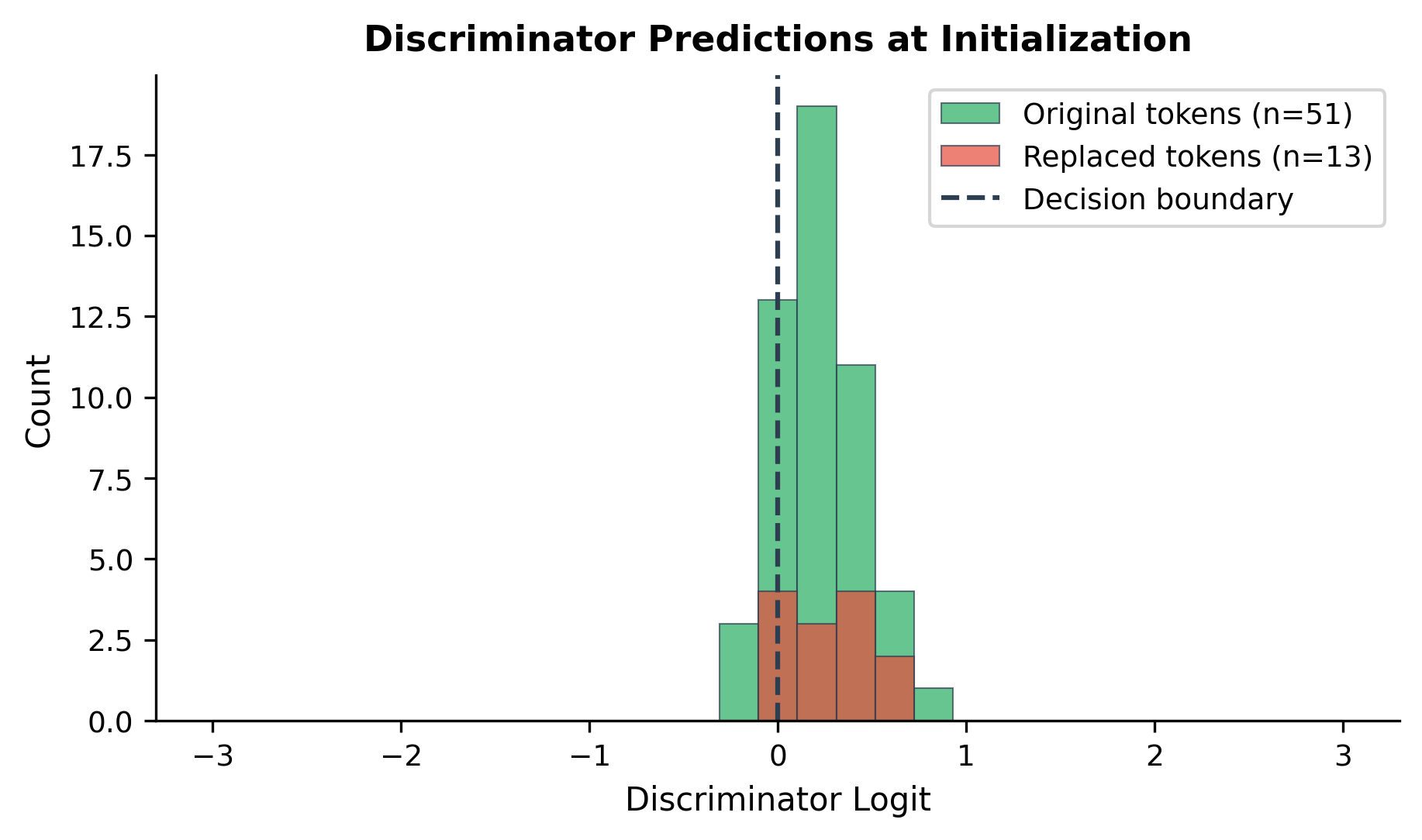
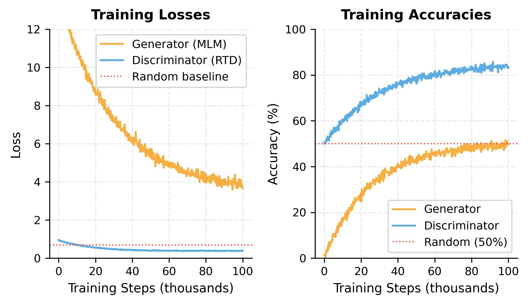
The discriminator has roughly 85M parameters, significantly larger than the generator. The replacement rate is lower than the 15% masking rate because the generator sometimes predicts the correct original token. The discriminator loss starts near the random baseline (0.69, which is log(2)\log(2) for binary classification), indicating the untrained model has no ability to distinguish original from replaced tokens.

Out[15]:
Visualization
Histogram showing overlapping distributions of discriminator logits for original and replaced tokens.
Discriminator prediction confidence distribution at initialization. The untrained discriminator outputs near-zero logits for both original and replaced tokens, unable to distinguish between them. After training, these distributions would separate with replaced tokens receiving positive logits and original tokens receiving negative logits.

Notice that the generator can produce the same token as the original. When it does, that position is not "replaced" even though it went through the generator. This means the actual replacement rate is typically lower than the masking rate. The discriminator learns to identify both truly replaced tokens and those where the generator happened to guess correctly.

The Replaced Token Detection Objective

The RTD objective trains the discriminator to predict is_replaced for every token. Let's formalize the setup before presenting the loss function.

Problem setup:

  • We start with an original sequence x=[x1,x2,,xn]\mathbf{x} = [x_1, x_2, \ldots, x_n] containing nn tokens
  • A random subset of positions M{1,,n}\mathcal{M} \subset \{1, \ldots, n\} is selected for masking (typically 15% of positions)
  • The generator receives the sequence with [MASK] tokens at positions in M\mathcal{M} and produces replacement tokens x~i\tilde{x}_i for each iMi \in \mathcal{M}
  • The corrupted sequence x~\tilde{\mathbf{x}} combines original and generated tokens: x~i=xi\tilde{x}_i = x_i for positions not in M\mathcal{M}, and x~i\tilde{x}_i equals the generator's sampled token for positions in M\mathcal{M}

Note that even at masked positions, the generator might sample the same token as the original. These positions are technically "original" for the discriminator's task, since no replacement occurred.

The discriminator outputs logits D(x~)iD(\tilde{\mathbf{x}})_i for each position. The RTD loss is the standard binary cross-entropy, summed across all positions in the sequence:

LRTD=i=1n[yilogσ(Di)+(1yi)log(1σ(Di))]\mathcal{L}_{\text{RTD}} = -\sum_{i=1}^{n} \left[ y_i \log \sigma(D_i) + (1 - y_i) \log (1 - \sigma(D_i)) \right]

where:

  • nn: the total number of tokens in the sequence (e.g., 512)
  • Di=D(x~)iD_i = D(\tilde{\mathbf{x}})_i: the discriminator's raw logit output at position ii, representing how confident the model is that the token was replaced
  • σ()\sigma(\cdot): the sigmoid function, which converts the logit to a probability between 0 and 1
  • yi=1[x~ixi]y_i = \mathbb{1}[\tilde{x}_i \neq x_i]: the ground truth label, equal to 1 if the token at position ii was replaced by the generator, and 0 if it's the original token

The loss decomposes into two cases: when yi=1y_i = 1 (token was replaced), the loss is logσ(Di)-\log \sigma(D_i), encouraging the model to output a high logit. When yi=0y_i = 0 (token is original), the loss is log(1σ(Di))-\log(1 - \sigma(D_i)), encouraging a low logit. The sum runs over all nn positions, not just the masked ones. This is the crucial difference from MLM: every token contributes to learning.

Out[16]:
Visualization
Side-by-side comparison showing MLM learning from sparse masked positions versus RTD learning from all positions.
Learning signal comparison between MLM and RTD. MLM learns from 15% of tokens (masked positions only), while RTD learns from 100% of tokens. This 6.7x increase in learning signal per batch explains ELECTRA's sample efficiency.

Joint Training

ELECTRA trains the generator and discriminator simultaneously. The total loss combines both objectives into a single scalar that drives gradient updates:

LELECTRA=LMLM+λLRTD\mathcal{L}_{\text{ELECTRA}} = \mathcal{L}_{\text{MLM}} + \lambda \mathcal{L}_{\text{RTD}}

where:

  • LMLM\mathcal{L}_{\text{MLM}}: the masked language modeling loss for the generator
  • LRTD\mathcal{L}_{\text{RTD}}: the replaced token detection loss for the discriminator
  • λ\lambda: a weighting factor (typically 50) that balances the two losses

The high weight on RTD ensures the discriminator is the primary focus of training. Without this upweighting, the generator's gradients would dominate because MLM involves a 30,000-way classification (much harder per token than binary classification).

The generator's MLM loss is computed only at masked positions:

LMLM=iMlogPG(xix~masked)\mathcal{L}_{\text{MLM}} = -\sum_{i \in \mathcal{M}} \log P_G(x_i \mid \tilde{\mathbf{x}}_{\text{masked}})

where:

  • M\mathcal{M}: the set of masked positions (typically 15% of sequence length)
  • xix_i: the original token at position ii (the target we want the generator to predict)
  • x~masked\tilde{\mathbf{x}}_{\text{masked}}: the input sequence with [MASK] tokens at positions in M\mathcal{M}
  • PG(xix~masked)P_G(x_i \mid \tilde{\mathbf{x}}_{\text{masked}}): the probability the generator assigns to the correct token xix_i given the masked input

This is standard cross-entropy loss: the generator is rewarded for assigning high probability to the original tokens at masked positions.

In[17]:
Code
def compute_generator_loss(gen_logits, original_ids, masked_positions):
    """
    Compute MLM loss for the generator.

    Args:
        gen_logits: (batch_size, seq_len, vocab_size)
        original_ids: (batch_size, seq_len) - original token IDs
        masked_positions: (batch_size, seq_len) - bool mask of masked positions

    Returns:
        Scalar loss
    """
    batch_size, seq_len, vocab_size = gen_logits.shape

    # Flatten for cross-entropy
    logits_flat = gen_logits.view(-1, vocab_size)
    labels_flat = original_ids.view(-1)
    mask_flat = masked_positions.view(-1)

    # Compute loss only at masked positions
    loss = F.cross_entropy(logits_flat, labels_flat, reduction="none")
    loss = (loss * mask_flat).sum() / mask_flat.sum()

    return loss


def electra_training_step(
    generator,
    discriminator,
    input_ids,
    mask_token_id,
    mask_prob=0.15,
    rtd_weight=50.0,
):
    """
    Complete ELECTRA training step.

    Returns:
        Dictionary with losses and statistics
    """
    # Step 1: Create masked input
    masked_ids, masked_positions = create_masked_input(
        input_ids, mask_token_id, mask_prob
    )

    # Step 2: Generator forward pass
    gen_logits = generator(masked_ids)
    gen_loss = compute_generator_loss(gen_logits, input_ids, masked_positions)

    # Step 3: Sample replacements (no gradient through sampling)
    with torch.no_grad():
        corrupted_ids = generator.sample_replacements(
            masked_ids, masked_positions
        )

    # Step 4: Determine which tokens differ from original
    is_replaced = (corrupted_ids != input_ids).long()

    # Step 5: Discriminator forward pass
    disc_logits = discriminator(corrupted_ids)
    disc_loss = compute_discriminator_loss(disc_logits, is_replaced)

    # Step 6: Combined loss
    total_loss = gen_loss + rtd_weight * disc_loss

    # Statistics
    with torch.no_grad():
        disc_preds = (disc_logits > 0).long()
        disc_accuracy = (disc_preds == is_replaced).float().mean()
        gen_accuracy = (
            (corrupted_ids == input_ids)[masked_positions].float().mean()
        )

    return {
        "total_loss": total_loss,
        "gen_loss": gen_loss,
        "disc_loss": disc_loss,
        "disc_accuracy": disc_accuracy,
        "gen_accuracy": gen_accuracy,
        "replacement_rate": is_replaced.float().mean(),
    }
In[18]:
Code
# Demonstrate a training step
torch.manual_seed(42)

# Reset models
generator = ElectraGenerator(
    vocab_size=30522,
    hidden_size=256,
    num_layers=4,
    num_heads=4,
    intermediate_size=1024,
)

discriminator = ElectraDiscriminator(
    vocab_size=30522,
    hidden_size=768,
    num_layers=12,
    num_heads=12,
    intermediate_size=3072,
)

# Sample input
input_ids = torch.randint(100, 1000, (4, 64))

# Training step
results = electra_training_step(
    generator, discriminator, input_ids, mask_token_id=103
)
Out[19]:
Console
ELECTRA Training Step Results:
  Generator loss: 10.5056
  Discriminator loss: 0.7005
  Total loss: 45.5294

Accuracies:
  Generator (predicting masked tokens): 0.0%
  Discriminator (detecting replacements): 48.8%

Replacement rate: 18.4%

At initialization, both networks perform near chance level: the generator accuracy is close to random guessing among 30,000 vocabulary tokens, and the discriminator accuracy hovers around 50% for binary classification. The generator loss is high (around 10, reflecting the log of vocab size), while the discriminator loss is near 0.69 (the random baseline for binary cross-entropy). During training, both losses decrease as the generator learns to predict masked tokens and the discriminator learns to detect replacements.

The λ=50\lambda = 50 weight is important and deserves explanation. The generator loss is computed over approximately 15% of tokens with a 30,000-way classification at each position, while the discriminator loss is computed over 100% of tokens but with only binary classification at each position.

The cross-entropy loss magnitude scales with the log of the number of classes: for MLM, this is approximately log(30000)10.3\log(30000) \approx 10.3 per position, while for RTD it's log(2)0.69\log(2) \approx 0.69 per position. Even though RTD has more positions, the per-position loss magnitude is much smaller. Without upweighting RTD, the MLM gradients would dominate the shared embeddings. The λ=50\lambda = 50 factor ensures both networks receive comparable gradient magnitudes, allowing the discriminator to learn effectively.

Out[20]:
Visualization
Bar chart comparing per-position loss magnitudes for MLM versus RTD objectives.
Loss magnitude comparison between MLM and RTD objectives. The MLM loss per position is approximately 15× larger than RTD due to the vocabulary size difference (30,000-way vs binary classification). The λ=50 weight compensates for this imbalance.

Why No Adversarial Training?

You might wonder why ELECTRA doesn't use adversarial training like a GAN. The generator could try to fool the discriminator, making training competitive rather than cooperative. The ELECTRA authors experimented with this and found it hurt performance.

The problem is the discreteness of text. GANs work well for continuous outputs (images, audio) where small gradient-based adjustments smoothly improve quality. Text is discrete: you either sample token 7842 or you don't. There's no gradient to flow back from the discriminator's judgment of that specific token choice.

Techniques like REINFORCE can estimate gradients through discrete sampling, but they introduce high variance. In ELECTRA's experiments, adversarial training with REINFORCE produced unstable training and worse results. The simple cooperative approach, where both networks minimize their own losses, proved more effective.
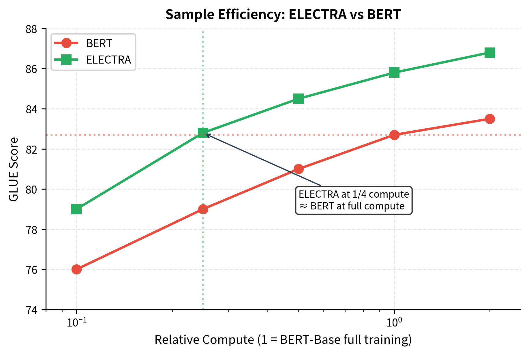
Out[21]:
Visualization
Diagram comparing cooperative and adversarial training paradigms with arrows showing gradient flow direction.
Cooperative versus adversarial training in ELECTRA. In cooperative training (used), both networks minimize their own losses. In adversarial training (not used), the generator tries to maximize the discriminator's loss. Cooperative training is more stable for discrete outputs like text.

Sample Efficiency

ELECTRA's main contribution is sample efficiency: it achieves the same performance as BERT with far less compute. The original paper demonstrated this across multiple scales.

At the small scale (comparable to BERT-Small with 14M parameters), ELECTRA trained for 1/4 of BERT's training steps matched BERT's full-training performance. At the base scale (110M parameters), ELECTRA trained with 1/4 the compute exceeded BERT's performance. At the large scale (335M parameters), ELECTRA achieved new state-of-the-art results on GLUE.

Out[22]:
Visualization
Line plot showing GLUE score versus compute FLOPs for BERT and ELECTRA, with ELECTRA consistently higher.
ELECTRA's sample efficiency compared to BERT. At each compute budget, ELECTRA achieves higher GLUE scores. With 1/4 the compute, ELECTRA matches BERT-Base performance. With equal compute, ELECTRA exceeds BERT by several points.

Why is ELECTRA so efficient? Three factors contribute:

  1. Learning from all tokens: RTD provides signal for every position, not just 15%. This roughly 6.7x increase in gradient information per batch directly translates to faster learning.

  2. Easier task per token: Binary classification is simpler than vocabulary prediction. The discriminator can focus its capacity on understanding context rather than memorizing rare vocabulary items.

  3. Generator bootstrapping: The small generator quickly learns to produce plausible replacements, providing meaningful training signal to the discriminator from early in training.

In[23]:
Code
def compare_learning_signal():
    """Compare gradient information per batch between MLM and RTD."""
    seq_len = 512
    mask_prob = 0.15
    vocab_size = 30522

    # MLM: gradient only from masked positions
    mlm_positions = int(seq_len * mask_prob)
    mlm_bits_per_position = np.log2(vocab_size)  # ~15 bits for 30k vocab
    mlm_total_bits = mlm_positions * mlm_bits_per_position

    # RTD: gradient from all positions
    rtd_positions = seq_len
    rtd_bits_per_position = 1  # binary classification
    rtd_total_bits = rtd_positions * rtd_bits_per_position

    return {
        "mlm_positions": mlm_positions,
        "mlm_bits_per_pos": mlm_bits_per_position,
        "mlm_total_bits": mlm_total_bits,
        "rtd_positions": rtd_positions,
        "rtd_bits_per_pos": rtd_bits_per_position,
        "rtd_total_bits": rtd_total_bits,
        "position_ratio": rtd_positions / mlm_positions,
    }
Out[24]:
Console
Learning Signal Comparison (per 512-token sequence):

MLM (BERT):
  Positions with gradient: 76
  Classification complexity: 14.9 bits (30k-way)
  Total information: 1132 bits

RTD (ELECTRA):
  Positions with gradient: 512
  Classification complexity: 1 bit (binary)
  Total information: 512 bits

Position coverage improvement: 6.7x

ELECTRA provides gradient signal at 6.7× more positions than MLM. While the per-position information content differs (15 bits for vocabulary prediction versus 1 bit for binary classification), the increased coverage more than compensates. The model receives learning signal from every token, not just the sparse masked positions.

The comparison isn't quite apples-to-apples because MLM's vocabulary-sized prediction is harder per position than RTD's binary classification. But the positions matter more than the per-position complexity: learning about context from 512 positions beats learning about vocabulary from 77 positions. The model needs to understand context to succeed at either task, and more positions means more context learning.

ELECTRA Scaling

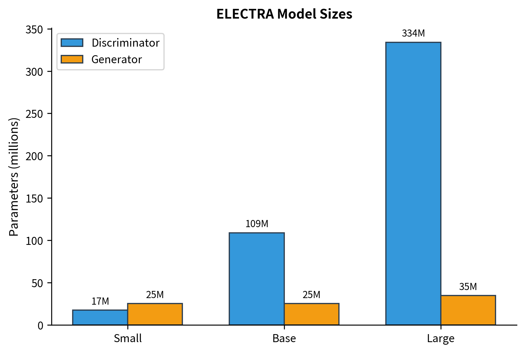
ELECTRA was released in three sizes: Small, Base, and Large. The configurations follow BERT's patterns but with the addition of a proportionally-sized generator.

In[25]:
Code
electra_configs = {
    "ELECTRA-Small": {
        "disc_hidden": 256,
        "disc_layers": 12,
        "disc_heads": 4,
        "disc_intermediate": 1024,
        "gen_hidden": 256,
        "gen_layers": 12,
        "gen_heads": 4,
        "gen_intermediate": 1024,
        "gen_fraction": 1.0,  # Same size as discriminator
    },
    "ELECTRA-Base": {
        "disc_hidden": 768,
        "disc_layers": 12,
        "disc_heads": 12,
        "disc_intermediate": 3072,
        "gen_hidden": 256,
        "gen_layers": 12,
        "gen_heads": 4,
        "gen_intermediate": 1024,
        "gen_fraction": 1 / 3,
    },
    "ELECTRA-Large": {
        "disc_hidden": 1024,
        "disc_layers": 24,
        "disc_heads": 16,
        "disc_intermediate": 4096,
        "gen_hidden": 256,
        "gen_layers": 24,
        "gen_heads": 4,
        "gen_intermediate": 1024,
        "gen_fraction": 1 / 4,
    },
}


def estimate_electra_params(config, vocab_size=30522):
    """Estimate parameters for ELECTRA configuration."""
    # Discriminator parameters
    disc_h = config["disc_hidden"]
    disc_l = config["disc_layers"]
    disc_i = config["disc_intermediate"]

    disc_embedding = vocab_size * disc_h + 512 * disc_h  # Token + position
    disc_attention = disc_l * (4 * disc_h * disc_h + 4 * disc_h)
    disc_ffn = disc_l * (disc_h * disc_i + disc_i + disc_i * disc_h + disc_h)
    disc_layernorm = disc_l * 4 * disc_h
    disc_head = disc_h + 1  # Binary classifier

    disc_total = (
        disc_embedding + disc_attention + disc_ffn + disc_layernorm + disc_head
    )

    # Generator parameters
    gen_h = config["gen_hidden"]
    gen_l = config["gen_layers"]
    gen_i = config["gen_intermediate"]

    gen_embedding = vocab_size * gen_h + 512 * gen_h
    gen_attention = gen_l * (4 * gen_h * gen_h + 4 * gen_h)
    gen_ffn = gen_l * (gen_h * gen_i + gen_i + gen_i * gen_h + gen_h)
    gen_layernorm = gen_l * 4 * gen_h
    gen_head = gen_h * vocab_size + vocab_size  # MLM head

    gen_total = (
        gen_embedding + gen_attention + gen_ffn + gen_layernorm + gen_head
    )

    return {
        "discriminator": disc_total,
        "generator": gen_total,
        "total": disc_total + gen_total,
        "disc_only": disc_total,  # What gets used for fine-tuning
    }
Out[26]:
Console
ELECTRA Model Configurations:
--------------------------------------------------------------------------------
Model              Disc Hidden  Gen Hidden   Disc Params    Total Params  
--------------------------------------------------------------------------------
ELECTRA-Small      256          256                17.4M         42.7M
ELECTRA-Base       768          256               108.9M        134.2M
ELECTRA-Large      1024         256               334.1M        368.8M

The discriminator size scales from ~14M parameters (Small) to ~335M (Large), matching BERT's configurations. The generator stays fixed at 256 hidden dimensions across all sizes, contributing only ~16M additional parameters. For downstream tasks, only the discriminator parameters matter. The generator is discarded after pre-training.

Notice that the generator is always small (256 hidden size) regardless of discriminator size. This is intentional. A small generator produces imperfect replacements that are challenging but not impossible for the discriminator. The generator parameters are discarded after pre-training; only the discriminator is used for downstream tasks.

Out[27]:
Visualization
Bar chart comparing discriminator and generator parameters across ELECTRA Small, Base, and Large configurations.
ELECTRA model sizes. The discriminator grows across configurations while the generator stays small. Only discriminator parameters matter for downstream tasks; generator parameters are discarded after pre-training.

Weight Sharing

ELECTRA can optionally share embeddings between the generator and discriminator. Since both networks process the same vocabulary, their token embeddings can be identical. This reduces total parameters and ensures consistent token representations.

When the generator and discriminator have different hidden sizes (as in ELECTRA-Base and Large), sharing requires a linear projection to map between sizes:

In[28]:
Code
class ElectraWithSharedEmbeddings(nn.Module):
    """ELECTRA with weight sharing between generator and discriminator."""

    def __init__(
        self,
        vocab_size,
        disc_hidden,
        gen_hidden,
        disc_layers,
        gen_layers,
        disc_heads,
        gen_heads,
        disc_intermediate,
        gen_intermediate,
        max_position=512,
        dropout=0.1,
    ):
        super().__init__()

        # Shared embeddings (in discriminator's hidden size)
        self.shared_token_embedding = nn.Embedding(vocab_size, disc_hidden)
        self.shared_position_embedding = nn.Embedding(max_position, disc_hidden)

        # Projection for generator if hidden sizes differ
        if gen_hidden != disc_hidden:
            self.gen_embedding_projection = nn.Linear(disc_hidden, gen_hidden)
        else:
            self.gen_embedding_projection = None

        # Generator components (without embeddings)
        self.gen_embedding_norm = nn.LayerNorm(gen_hidden)
        self.gen_embedding_dropout = nn.Dropout(dropout)

        gen_layer = nn.TransformerEncoderLayer(
            d_model=gen_hidden,
            nhead=gen_heads,
            dim_feedforward=gen_intermediate,
            dropout=dropout,
            activation="gelu",
            batch_first=True,
        )
        self.gen_encoder = nn.TransformerEncoder(gen_layer, gen_layers)

        self.gen_mlm_dense = nn.Linear(gen_hidden, gen_hidden)
        self.gen_mlm_norm = nn.LayerNorm(gen_hidden)
        self.gen_mlm_output = nn.Linear(gen_hidden, vocab_size)

        # Discriminator components (without embeddings)
        self.disc_embedding_norm = nn.LayerNorm(disc_hidden)
        self.disc_embedding_dropout = nn.Dropout(dropout)

        disc_layer = nn.TransformerEncoderLayer(
            d_model=disc_hidden,
            nhead=disc_heads,
            dim_feedforward=disc_intermediate,
            dropout=dropout,
            activation="gelu",
            batch_first=True,
        )
        self.disc_encoder = nn.TransformerEncoder(disc_layer, disc_layers)

        self.disc_head = nn.Linear(disc_hidden, 1)

        self.vocab_size = vocab_size

    def get_embeddings(self, input_ids, for_generator=False):
        """Get embeddings, with optional projection for generator."""
        batch_size, seq_len = input_ids.shape
        positions = torch.arange(seq_len, device=input_ids.device).unsqueeze(0)

        x = self.shared_token_embedding(input_ids)
        x = x + self.shared_position_embedding(positions)

        if for_generator and self.gen_embedding_projection is not None:
            x = self.gen_embedding_projection(x)

        return x

    def generator_forward(self, input_ids):
        """Forward pass through generator."""
        x = self.get_embeddings(input_ids, for_generator=True)
        x = self.gen_embedding_norm(x)
        x = self.gen_embedding_dropout(x)
        x = self.gen_encoder(x)

        x = self.gen_mlm_dense(x)
        x = F.gelu(x)
        x = self.gen_mlm_norm(x)
        logits = self.gen_mlm_output(x)

        return logits

    def discriminator_forward(self, input_ids):
        """Forward pass through discriminator."""
        x = self.get_embeddings(input_ids, for_generator=False)
        x = self.disc_embedding_norm(x)
        x = self.disc_embedding_dropout(x)
        x = self.disc_encoder(x)

        logits = self.disc_head(x).squeeze(-1)

        return logits

Weight sharing introduces a subtle issue. If we backpropagate through both networks simultaneously, the shared embeddings receive gradients from both the MLM loss (via generator) and the RTD loss (via discriminator). The ELECTRA paper found this works well, with the discriminator's gradients dominating due to the higher RTD weight and the learning from all positions.

Out[29]:
Visualization
Line plots showing generator and discriminator loss curves over training steps, demonstrating the co-training dynamics.
Simulated ELECTRA training dynamics. The generator loss decreases as it learns to predict masked tokens, while the discriminator loss first decreases then stabilizes as the generator improves. Generator accuracy rises quickly, making the discriminator's task progressively harder.

Fine-tuning ELECTRA

After pre-training, the generator is discarded. Only the discriminator is used for downstream tasks. Fine-tuning follows the same pattern as BERT: add a task-specific head and train on labeled data.

For classification tasks, the [CLS] token representation from the discriminator feeds into a classification layer:

In[30]:
Code
class ElectraForSequenceClassification(nn.Module):
    """ELECTRA discriminator with classification head."""

    def __init__(self, discriminator, num_labels, dropout=0.1):
        super().__init__()
        self.discriminator = discriminator

        # Remove the RTD head
        hidden_size = discriminator.token_embedding.embedding_dim

        # Add classification head
        self.dropout = nn.Dropout(dropout)
        self.classifier = nn.Linear(hidden_size, num_labels)

    def forward(self, input_ids, attention_mask=None, labels=None):
        batch_size, seq_len = input_ids.shape

        # Get discriminator embeddings
        positions = torch.arange(seq_len, device=input_ids.device).unsqueeze(0)
        x = self.discriminator.token_embedding(input_ids)
        x = x + self.discriminator.position_embedding(positions)
        x = self.discriminator.embedding_norm(x)
        x = self.discriminator.embedding_dropout(x)

        # Create mask
        if attention_mask is not None:
            src_key_padding_mask = attention_mask == 0
        else:
            src_key_padding_mask = None

        # Encode
        x = self.discriminator.encoder(
            x, src_key_padding_mask=src_key_padding_mask
        )

        # Classification from [CLS] token (position 0)
        cls_output = x[:, 0]
        cls_output = self.dropout(cls_output)
        logits = self.classifier(cls_output)

        loss = None
        if labels is not None:
            loss = F.cross_entropy(logits, labels)

        return {"loss": loss, "logits": logits}

For token-level tasks like NER or question answering, we use the full sequence output instead of just [CLS]:

In[31]:
Code
class ElectraForTokenClassification(nn.Module):
    """ELECTRA discriminator with token classification head."""

    def __init__(self, discriminator, num_labels, dropout=0.1):
        super().__init__()
        self.discriminator = discriminator

        hidden_size = discriminator.token_embedding.embedding_dim

        self.dropout = nn.Dropout(dropout)
        self.classifier = nn.Linear(hidden_size, num_labels)

    def forward(self, input_ids, attention_mask=None, labels=None):
        batch_size, seq_len = input_ids.shape

        # Get discriminator embeddings
        positions = torch.arange(seq_len, device=input_ids.device).unsqueeze(0)
        x = self.discriminator.token_embedding(input_ids)
        x = x + self.discriminator.position_embedding(positions)
        x = self.discriminator.embedding_norm(x)
        x = self.discriminator.embedding_dropout(x)

        if attention_mask is not None:
            src_key_padding_mask = attention_mask == 0
        else:
            src_key_padding_mask = None

        x = self.discriminator.encoder(
            x, src_key_padding_mask=src_key_padding_mask
        )

        # Classification for all tokens
        x = self.dropout(x)
        logits = self.classifier(x)

        loss = None
        if labels is not None:
            loss = F.cross_entropy(
                logits.view(-1, logits.size(-1)), labels.view(-1)
            )

        return {"loss": loss, "logits": logits}

One consideration for fine-tuning: ELECTRA's pre-training teaches the model to detect replaced tokens, not to understand [MASK] tokens. This means ELECTRA doesn't have the pretrain-finetune mismatch that affects BERT (where [MASK] appears in pre-training but not fine-tuning). The discriminator always sees real tokens, both during pre-training and fine-tuning.

Using Pre-trained ELECTRA

In practice, you'll load pre-trained ELECTRA models from Hugging Face rather than training from scratch:

In[32]:
Code
from transformers import ElectraTokenizer, ElectraModel

# Load pre-trained ELECTRA
tokenizer = ElectraTokenizer.from_pretrained(
    "google/electra-small-discriminator"
)
model = ElectraModel.from_pretrained("google/electra-small-discriminator")
model.eval()

# Prepare input
text = "ELECTRA learns efficiently by detecting replaced tokens."
inputs = tokenizer(text, return_tensors="pt")
Out[33]:
Console
Input text: ELECTRA learns efficiently by detecting replaced tokens.
Token IDs: [101, 11322, 2527, 10229, 18228, 2011, 25952, 2999, 19204, 2015, 1012, 102]
Tokens: ['[CLS]', 'elect', '##ra', 'learns', 'efficiently', 'by', 'detecting', 'replaced', 'token', '##s', '.', '[SEP]']

The tokenizer adds special tokens ([CLS] at the start, [SEP] at the end) and splits words using WordPiece. Notice that "efficiently" becomes "efficient" + "##ly". The ## prefix indicates a subword continuation.

In[34]:
Code
# Get hidden states
with torch.no_grad():
    outputs = model(**inputs)
    hidden_states = outputs.last_hidden_state
Out[35]:
Console
Hidden states shape: torch.Size([1, 12, 256])
  - Batch size: 1, Sequence length: 12, Hidden dimension: 256

CLS embedding (first 10 dims): [-0.13447017967700958, 0.18001484870910645, -0.5841339826583862, 0.3974248766899109, -0.09176717698574066, 0.020525239408016205, 0.7062873840332031, 1.0155174732208252, 0.9312728643417358, -0.17594000697135925]

The model outputs a 256-dimensional vector for each token (ELECTRA-Small's hidden size). The [CLS] token's representation at position 0 aggregates information from the entire sequence and is typically used for classification tasks.

For classification tasks, use the task-specific model directly:

In[36]:
Code
from transformers import (
    ElectraForSequenceClassification as HFElectraForSequenceClassification,
)

# For sentiment classification
classifier = HFElectraForSequenceClassification.from_pretrained(
    "google/electra-small-discriminator",
    num_labels=2,  # Binary classification
)
classifier.eval()

with torch.no_grad():
    outputs = classifier(**inputs)
    logits = outputs.logits
    probs = F.softmax(logits, dim=-1)
Out[37]:
Console
Classification output:
  Logits: [0.0374, -0.0296]
  Probabilities: [0.5167, 0.4833]
  Predicted class: 0

The probabilities are close to 50/50, which is expected: the classification head was randomly initialized and hasn't been fine-tuned on any labeled data. After fine-tuning on a sentiment dataset (like SST-2), the model would produce meaningful, confident predictions.

Note that the untrained classification head produces random outputs. After fine-tuning on a sentiment dataset, the model would produce meaningful predictions.

Performance Comparison

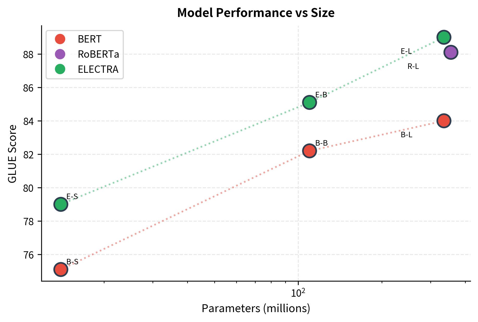
ELECTRA's results on standard benchmarks demonstrate its efficiency. Here's a comparison with BERT and RoBERTa at various scales:

In[38]:
Code
# Approximate results from ELECTRA paper
benchmark_results = {
    "BERT-Small": {"params": 14, "glue_avg": 75.1, "squad_v2": 68.2},
    "ELECTRA-Small": {"params": 14, "glue_avg": 79.0, "squad_v2": 74.8},
    "BERT-Base": {"params": 110, "glue_avg": 82.2, "squad_v2": 76.3},
    "ELECTRA-Base": {"params": 110, "glue_avg": 85.1, "squad_v2": 80.5},
    "BERT-Large": {"params": 335, "glue_avg": 84.0, "squad_v2": 81.9},
    "RoBERTa-Large": {"params": 355, "glue_avg": 88.1, "squad_v2": 86.5},
    "ELECTRA-Large": {"params": 335, "glue_avg": 89.0, "squad_v2": 88.0},
}
Out[39]:
Console
Benchmark Results Comparison:
-----------------------------------------------------------------
Model              Parameters   GLUE Avg     SQuAD v2.0  
-----------------------------------------------------------------
BERT-Small               14M       75.1         68.2
ELECTRA-Small            14M       79.0         74.8
BERT-Base               110M       82.2         76.3
ELECTRA-Base            110M       85.1         80.5
BERT-Large              335M       84.0         81.9
RoBERTa-Large           355M       88.1         86.5
ELECTRA-Large           335M       89.0         88.0

The results reveal ELECTRA's remarkable efficiency. At each parameter budget, ELECTRA outperforms BERT by 3-4 points on GLUE. Most striking is ELECTRA-Small: with just 14M parameters, it achieves 79.0 on GLUE, comparable to BERT-Base at 110M parameters. This 8× parameter reduction with similar performance demonstrates that sample efficiency translates directly to model efficiency.

ELECTRA-Small outperforms BERT-Base despite having 8x fewer parameters. ELECTRA-Base exceeds RoBERTa-Base's performance. ELECTRA-Large achieves new state-of-the-art results on GLUE, exceeding RoBERTa-Large despite slightly fewer parameters.

Out[40]:
Visualization
Grouped bar chart comparing GLUE and SQuAD scores across BERT and ELECTRA models of various sizes.
Benchmark performance comparison. ELECTRA consistently outperforms BERT at each model size. ELECTRA-Small even exceeds BERT-Base performance with 8x fewer parameters, demonstrating exceptional parameter efficiency.

Limitations and Impact

ELECTRA's design comes with trade-offs worth understanding.

The generator must strike a balance between too good and too bad. If the generator produces perfect replacements, the discriminator receives no learning signal because all tokens look original. If the generator is random, replacements are trivially detectable and the discriminator learns little about language. The solution of using a small generator works but adds a hyperparameter (generator size relative to discriminator) that requires tuning.

Pre-training is more complex than BERT. Two networks, two losses, sampling from the generator, and the RTD weight all need coordination. Debugging is harder because problems might arise from either network or their interaction. The implementation overhead is real, though not prohibitive.

The generator parameters are wasted after pre-training. During training, compute is split between generator and discriminator, but only the discriminator matters for downstream tasks. The ELECTRA paper argues this is worthwhile because the generator is small (1/4 to 1/3 discriminator size) and the efficiency gains outweigh the cost.

Despite these limitations, ELECTRA's impact on the field was significant. It demonstrated that MLM's inefficiency wasn't inherent to pre-training but rather a design choice that could be improved. The replaced token detection paradigm influenced subsequent models and showed that creative objective design matters as much as architecture or scale. ELECTRA remains one of the most parameter-efficient pre-training approaches, particularly valuable when compute is limited.

Key Parameters

When implementing or fine-tuning ELECTRA, these parameters matter most:

  • mask_prob (default: 0.15): Fraction of tokens masked for generator input. Follows BERT's 15% rate. Higher rates create more replaced tokens but may make generator predictions less accurate.

  • rtd_weight (default: 50): Weight on discriminator loss relative to generator loss. The high weight ensures discriminator gradients dominate shared embeddings. Lower weights may cause generator to overfit.

  • generator_size_fraction (default: 0.25 to 0.33): Generator hidden size relative to discriminator. Smaller generators produce less accurate replacements, creating harder but more varied training signal.

  • temperature (default: 1.0): Sampling temperature for generator. Higher temperatures increase diversity of replacements. Lower temperatures produce more likely tokens, which may be too easy to detect.

  • learning_rate (default: 2e-4 for ELECTRA-Base): Both networks use the same learning rate. The standard BERT learning rate works well.

  • weight_sharing (default: True for embeddings): Whether generator and discriminator share token embeddings. Reduces parameters and ensures consistent token representations.

  • max_seq_length (default: 512): Maximum sequence length. ELECTRA uses full 512 throughout training, unlike BERT's phased approach.

Summary

ELECTRA reimagines pre-training by replacing masked language modeling with replaced token detection:

  • Two-network architecture: A small generator creates plausible token replacements for masked positions. A larger discriminator learns to detect which tokens were swapped.

  • Sample efficiency: By learning from every token position (not just 15% masked ones), ELECTRA achieves BERT's performance with 1/4 the compute. Given equal resources, it significantly exceeds BERT.

  • Cooperative training: Unlike GANs, both networks minimize their own losses rather than competing. This avoids gradient estimation problems for discrete text.

  • Generator size matters: The generator should be small enough to make mistakes but good enough for those mistakes to be plausible. This sweet spot provides optimal training signal.

  • Fine-tuning simplicity: Only the discriminator is used for downstream tasks. Fine-tuning follows the standard BERT pattern with no [MASK] token mismatch.

  • State-of-the-art efficiency: ELECTRA-Small outperforms BERT-Base despite 8x fewer parameters. ELECTRA-Large achieves the best GLUE results among comparably-sized models.

ELECTRA demonstrates that pre-training objective design matters as much as architecture scale. By learning from every token, it extracts maximum value from each training batch, making it particularly valuable when compute is limited.

Quiz

Ready to test your understanding? Take this quick quiz to reinforce what you've learned about ELECTRA's efficient pre-training approach.

Loading component...
Track your reading progress

Sign in to mark chapters as read and track your learning journey

Sign in →

Comments

Reference

BIBTEXAcademic
@misc{electraefficientpretrainingwithreplacedtokendetection, author = {Michael Brenndoerfer}, title = {ELECTRA: Efficient Pre-training with Replaced Token Detection}, year = {2025}, url = {https://mbrenndoerfer.com/writing/electra-efficient-pretraining-replaced-token-detection}, organization = {mbrenndoerfer.com}, note = {Accessed: 2025-12-19} }
APAAcademic
Michael Brenndoerfer (2025). ELECTRA: Efficient Pre-training with Replaced Token Detection. Retrieved from https://mbrenndoerfer.com/writing/electra-efficient-pretraining-replaced-token-detection
MLAAcademic
Michael Brenndoerfer. "ELECTRA: Efficient Pre-training with Replaced Token Detection." 2025. Web. 12/19/2025. <https://mbrenndoerfer.com/writing/electra-efficient-pretraining-replaced-token-detection>.
CHICAGOAcademic
Michael Brenndoerfer. "ELECTRA: Efficient Pre-training with Replaced Token Detection." Accessed 12/19/2025. https://mbrenndoerfer.com/writing/electra-efficient-pretraining-replaced-token-detection.
HARVARDAcademic
Michael Brenndoerfer (2025) 'ELECTRA: Efficient Pre-training with Replaced Token Detection'. Available at: https://mbrenndoerfer.com/writing/electra-efficient-pretraining-replaced-token-detection (Accessed: 12/19/2025).
SimpleBasic
Michael Brenndoerfer (2025). ELECTRA: Efficient Pre-training with Replaced Token Detection. https://mbrenndoerfer.com/writing/electra-efficient-pretraining-replaced-token-detection
Michael Brenndoerfer

About the author: Michael Brenndoerfer

All opinions expressed here are my own and do not reflect the views of my employer.

Michael currently works as an Associate Director of Data Science at EQT Partners in Singapore, leading AI and data initiatives across private capital investments.

With over a decade of experience spanning private equity, management consulting, and software engineering, he specializes in building and scaling analytics capabilities from the ground up. He has published research in leading AI conferences and holds expertise in machine learning, natural language processing, and value creation through data.

Stay updated

Get notified when I publish new articles on data and AI, private equity, technology, and more.

No spam, unsubscribe anytime.

or

Create a free account to unlock exclusive features, track your progress, and join the conversation.

No popupsUnobstructed readingCommenting100% Free