

Explore the BERT architecture in detail covering model sizes (Base vs Large), three-layer embedding system, bidirectional attention patterns, and output representations for downstream tasks.

This article is part of the free-to-read Language AI Handbook
Choose your expertise level to adjust how many terms are explained. Beginners see more tooltips, experts see fewer to maintain reading flow. Hover over underlined terms for instant definitions.
BERT Architecture
In October 2018, Google released a paper titled "BERT: Pre-training of Deep Bidirectional Transformers for Language Understanding." Within months, BERT had shattered performance records on eleven NLP benchmarks and fundamentally changed how the field approached language understanding tasks. The architecture that made this possible wasn't revolutionary in its components: it stacked transformer encoder blocks with multi-head self-attention and feed-forward networks. The revolution lay in how these familiar pieces were configured, trained, and applied.
This chapter examines the BERT architecture in detail. We'll explore the two model sizes (Base and Large) and their layer configurations, understand how BERT's three embedding types combine to represent input, examine the bidirectional attention patterns that distinguish BERT from autoregressive models, and analyze the output representations that downstream tasks use. By the end, you'll understand not just what BERT's architecture looks like, but why each design choice matters.
Model Sizes: Base vs Large
BERT comes in two standard configurations: BERT-Base and BERT-Large. These sizes were chosen deliberately to balance capability against practical deployment constraints. BERT-Base matches the hidden dimension of OpenAI's GPT (768), enabling direct comparisons, while BERT-Large pushes scale to demonstrate that larger models capture more nuanced language patterns.
BERT-Base contains 12 transformer encoder layers with 12 attention heads and a hidden dimension of 768, totaling approximately 110 million parameters. BERT-Large doubles the layers to 24, increases heads to 16, and expands the hidden dimension to 1024, reaching approximately 340 million parameters.
The architectural specifications for each variant are:
| Parameter | BERT-Base | BERT-Large |
|---|---|---|
| Layers () | 12 | 24 |
| Hidden size () | 768 | 1024 |
| Attention heads () | 12 | 16 |
| Head dimension () | 64 | 64 |
| Feed-forward size | 3072 | 4096 |
| Vocabulary size | 30,522 | 30,522 |
| Max sequence length | 512 | 512 |
| Parameters | ~110M | ~340M |
Notice that the head dimension remains constant at 64 across both variants. This means BERT-Large achieves more capacity by having more heads (16 vs 12) and more layers (24 vs 12), not by making each head larger. The feed-forward dimension follows the standard 4x multiplier relative to hidden size (768 × 4 = 3072 for Base, 1024 × 4 = 4096 for Large).
Let's compute the exact parameter counts to understand where capacity resides:
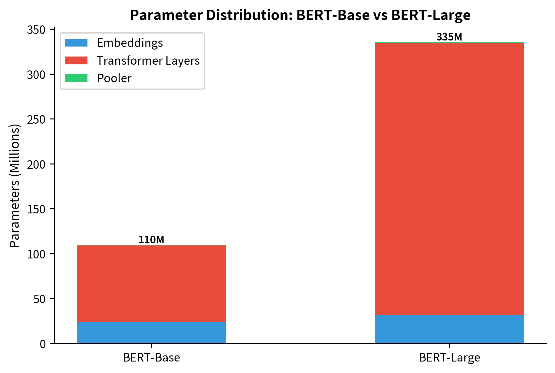
The vast majority of parameters reside in the transformer layers, particularly in the feed-forward networks. Token embeddings represent a significant portion due to the large vocabulary, but their contribution decreases proportionally as model depth increases. This distribution matters for understanding where BERT stores knowledge: factual information tends to concentrate in feed-forward weights, while attention patterns encode syntactic and semantic relationships.
The Input Representation
BERT's input representation is one of its most distinctive features. Unlike simpler models that use only token embeddings, BERT combines three embedding types to capture different aspects of the input. This design enables BERT to process sentence pairs for tasks like question answering and natural language inference.
Three Embedding Layers
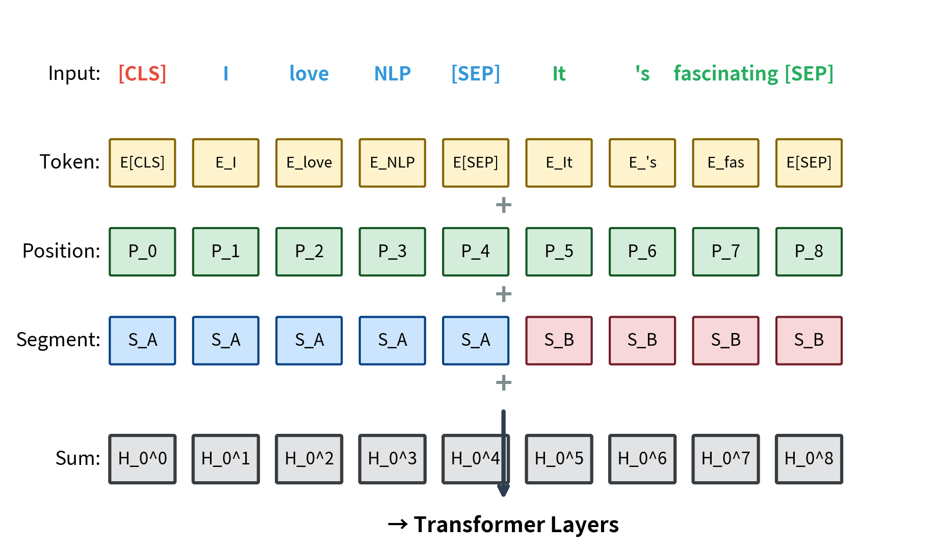
Every input token receives three embeddings that are summed together:
- Token embeddings: Standard learned embeddings that map each vocabulary token to a dense vector
- Position embeddings: Learned embeddings for each position (0 to 511) encoding sequential order
- Segment embeddings: Two learned embeddings (A and B) indicating which sentence a token belongs to
The segment embeddings deserve special attention. BERT was designed for tasks involving sentence pairs: given two sentences, determine if the second follows the first (next sentence prediction), if the first entails the second (natural language inference), or find the answer span (question answering). The segment embeddings allow the model to distinguish which tokens belong to which sentence even after they're concatenated.
Special Tokens
BERT uses several special tokens to structure its input:
- [CLS]: Prepended to every input. Its final representation is used for classification tasks
- [SEP]: Inserted between sentences and at the end of the input to mark boundaries
- [MASK]: Used during pretraining to indicate positions the model should predict
- [PAD]: Fills sequences shorter than the batch maximum length
- [UNK]: Represents tokens not in the vocabulary
Let's implement the embedding layer to see how these components combine:
The embedding layer transforms our 8-token input into a tensor of shape (1, 8, 768), where each token now has a 768-dimensional representation combining its identity, position, and segment information. This dense representation is what flows through the subsequent transformer layers.
The element-wise addition of three embedding types may seem unusual. Why not concatenate them? The answer lies in parameter efficiency and training dynamics. Addition keeps the hidden dimension fixed at 768, while concatenation would triple it. More subtly, addition forces the model to learn representations where token meaning, positional information, and segment identity can coexist in the same vector space. The layer normalization after addition rescales these combined representations to have consistent statistics.
Learned vs Sinusoidal Positions
BERT uses learned position embeddings rather than the sinusoidal encodings from the original transformer. Each of the 512 possible positions gets its own learned vector. This choice trades generalization for expressiveness: learned embeddings cannot extrapolate to positions beyond 512, but they can capture position-specific patterns that sinusoidal encodings cannot.
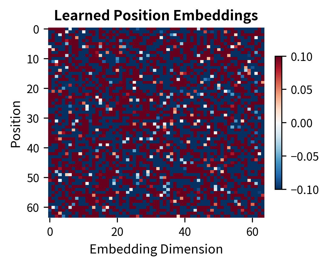
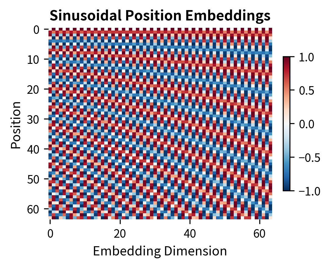
The learned embeddings appear less regular because they capture whatever positional patterns help with the pretraining objectives. The sinusoidal pattern's mathematical regularity means positions can be expressed as linear combinations of other positions, enabling some length generalization. BERT prioritized expressiveness over extrapolation since most downstream tasks don't require sequences longer than 512 tokens.
Transformer Encoder Layers
The core of BERT consists of stacked transformer encoder blocks. Each block applies multi-head self-attention followed by a position-wise feed-forward network, with residual connections and layer normalization around each sub-layer.
Layer Structure
Each transformer layer follows a consistent pattern:
- Multi-head self-attention with residual connection
- Layer normalization
- Feed-forward network with residual connection
- Layer normalization
BERT uses "post-norm" architecture, where layer normalization follows each sub-layer rather than preceding it. This differs from the "pre-norm" variant used in some later models like GPT-2.
The attention computation follows the standard scaled dot-product formula. Given query, key, and value matrices, attention computes a weighted combination of values where the weights depend on query-key similarity:
where:
- : the query matrix with shape (sequence length, head dimension), representing what each position is "looking for"
- : the key matrix with shape (sequence length, head dimension), representing what each position "offers" for matching
- : the value matrix with shape (sequence length, head dimension), containing the information to aggregate
- : the transpose of , enabling the matrix multiplication that produces similarity scores
- : the head dimension (64 in BERT), used for scaling
- : the scaling factor that prevents dot products from growing too large
- : normalizes scores to a probability distribution over positions
The scaling by is crucial for training stability. Without it, the dot products grow in magnitude with the dimension, pushing the softmax into regions where gradients vanish. With 64-dimensional heads, dot products could easily reach values of 8-10, making the softmax output nearly one-hot and preventing gradient flow.
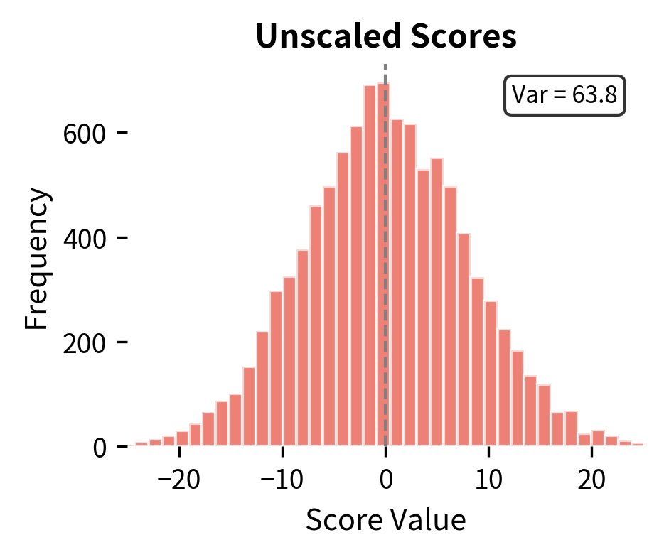
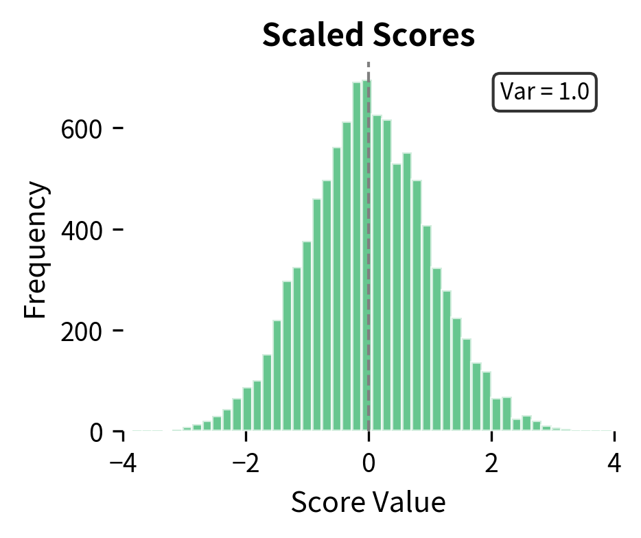
The histograms above demonstrate this effect. Raw dot products of 64-dimensional vectors have variance around 64, producing scores that span a wide range. After dividing by , the variance drops to approximately 1, keeping scores in a range where softmax produces meaningful probability distributions rather than near-deterministic outputs.
Feed-Forward Network
Each layer's feed-forward network expands the representation to 4x the hidden dimension, applies a non-linearity, then projects back:
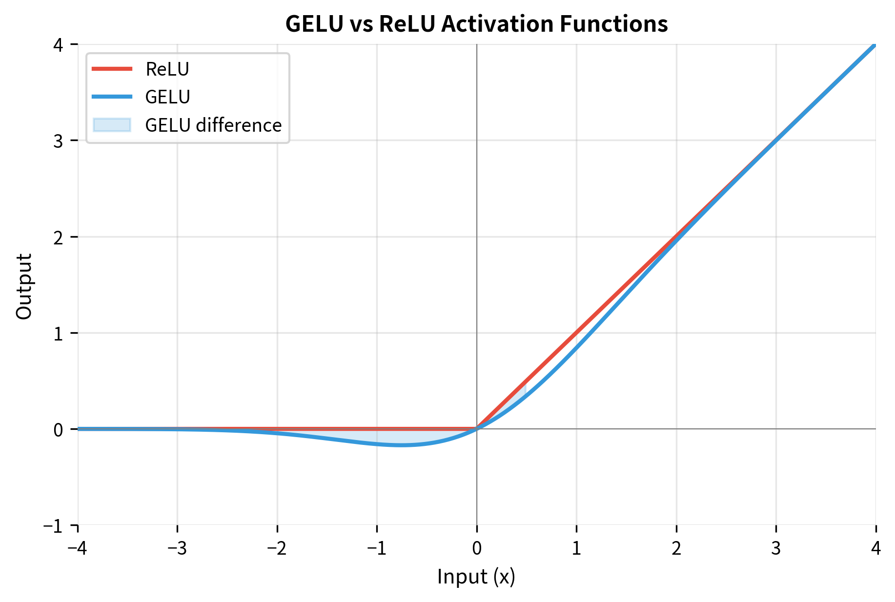
BERT uses GELU (Gaussian Error Linear Unit) activation rather than ReLU. GELU provides a smooth approximation to the gating mechanism, allowing small negative values to pass through while still providing non-linearity. The function can be understood as multiplying each input by the probability that a standard normal random variable would be less than that input:
where:
- : the input value to the activation function
- : the cumulative distribution function (CDF) of the standard normal distribution, giving the probability that a standard normal random variable is less than
- : the error function, a mathematical function related to the normal distribution's CDF
- : a scaling constant that converts from the standard error function to the normal CDF
Unlike ReLU, which abruptly zeroes out all negative inputs, GELU provides a smooth transition. For large positive , , so GELU. For large negative , , so GELU. The smooth transition around zero means small negative values can still contribute, which empirically improves training dynamics in transformer models.
Complete Encoder Layer
Combining attention and feed-forward with residual connections and layer normalization:
The layer maintains the same tensor shape between input and output, which is essential for stacking layers and enabling residual connections. The attention probabilities tensor shows dimensions for batch, heads, and both query and key positions, confirming that each of the 12 heads computes its own attention pattern over the sequence.
The residual connections are crucial for training deep networks. They allow gradients to flow directly backward through the network, mitigating the vanishing gradient problem. Without residuals, training a 12 or 24-layer network would be extremely difficult.
Bidirectional Attention Patterns
BERT's attention is bidirectional: every token can attend to every other token in the sequence. This contrasts sharply with the causal (left-to-right) attention used in GPT and other autoregressive models. The difference has profound implications for what patterns BERT can learn.
Visualizing Attention
Let's examine what attention patterns look like in practice. We'll create sample attention weights and visualize how different heads might specialize:
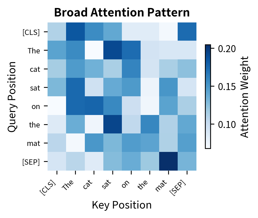
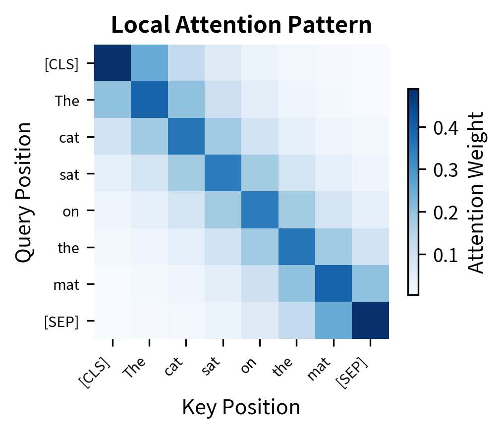
Research on BERT's attention patterns reveals consistent specialization:
- Early layers tend to attend broadly, with some heads focusing on the [CLS] token
- Middle layers develop syntactic patterns, with heads tracking subject-verb relationships, dependency arcs, and constituent boundaries
- Later layers show more semantic attention, with heads focusing on semantically related tokens
Attention Mask for Padding
When processing batches of variable-length sequences, BERT uses attention masks to prevent attending to padding tokens. The mask is applied as a large negative value before softmax, effectively zeroing out attention to padded positions:
The large negative value (-10000) becomes approximately zero after softmax, ensuring padded positions receive no attention weight.
Output Representations
BERT produces contextualized representations at every position. Different downstream tasks use these representations in different ways.
The [CLS] Token
The [CLS] token's final hidden state is designed to aggregate sequence-level information. During pretraining with the Next Sentence Prediction task, the [CLS] representation must contain enough information to determine whether two sentences are consecutive. This encourages [CLS] to capture global semantic content.
For classification tasks, you typically pass the [CLS] representation through a task-specific linear layer:
Token-Level Representations
For sequence labeling tasks like named entity recognition or part-of-speech tagging, you use the representation at each token position:
Span Representations
For extractive question answering, BERT predicts start and end positions of the answer span. Two linear layers project each token's representation to start and end logits:
Each head produces output with the appropriate shape for its task. The classification head reduces the sequence to a single prediction per sample. The token classification head produces a label prediction for each position. The QA head generates start and end scores for every token, allowing span extraction by finding the highest-scoring start-end pair.
The flexibility of BERT's output representations is key to its success. The same pretrained model can power classification, sequence labeling, question answering, and many other tasks by simply changing the task-specific head.
The Complete BERT Model
Let's assemble all components into a complete BERT implementation:
Our implementation produces approximately 85 million parameters, which is lower than the full 110M of BERT-Base because we omit the masked language modeling head and some auxiliary components. The model processes a batch of 2 sequences with 32 tokens each, producing contextualized representations at every position plus a pooled representation for sequence-level tasks.
Practical Considerations
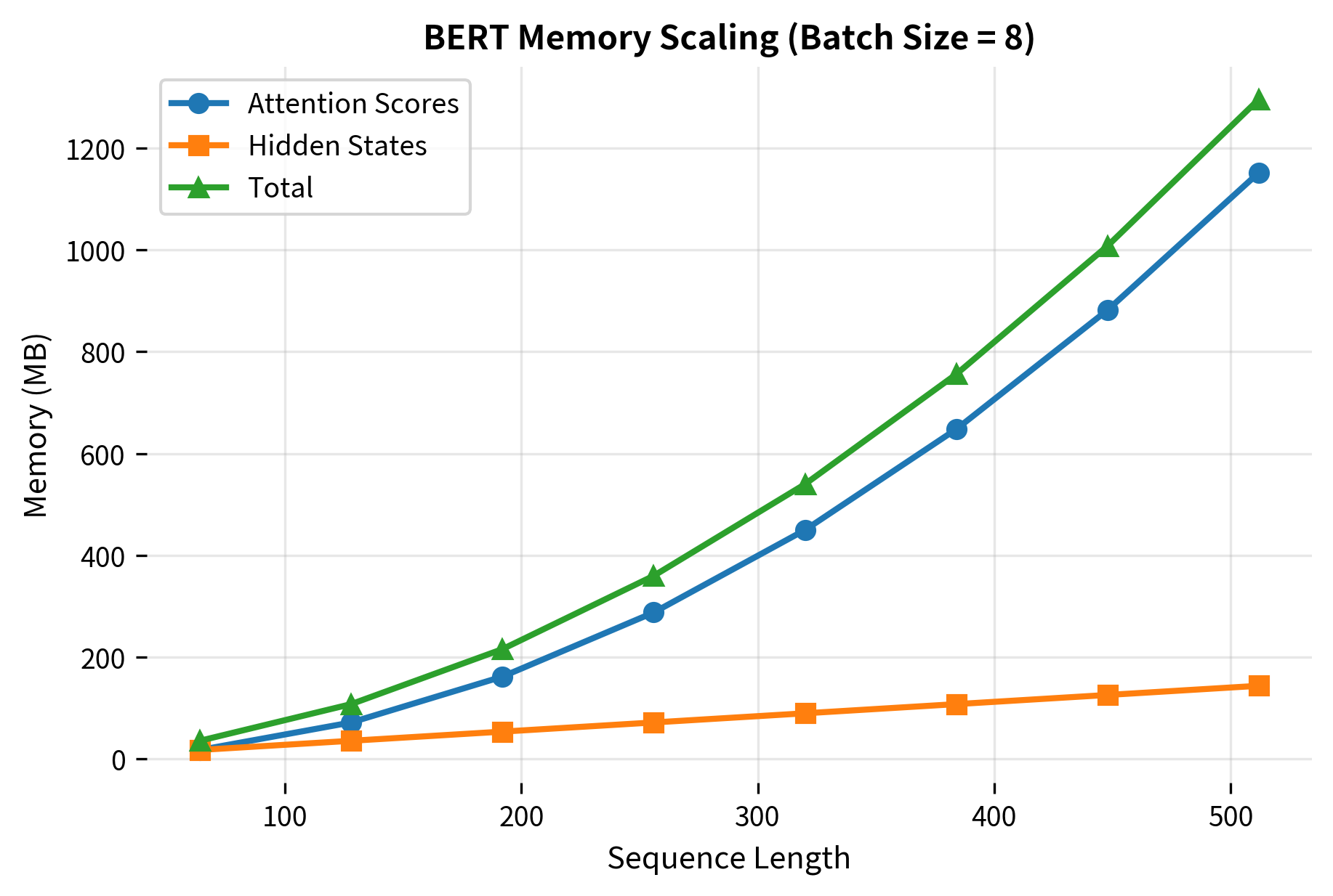
When deploying BERT, two factors dominate resource requirements: memory consumption and computational cost. Both scale with sequence length, making long documents particularly expensive to process.
Memory Requirements
BERT's memory usage during inference scales with sequence length squared due to the attention mechanism. For a batch of sequences, the dominant terms are:
- Embeddings:
- Attention scores:
- Intermediate activations:
For BERT-Base with a sequence length of 512 and batch size of 1, the attention scores alone require approximately 12 × 512 × 512 × 4 bytes (float32) = 12.6 MB per layer, or about 150 MB for all 12 layers.
Computational Complexity
The computational complexity of BERT is dominated by three operations:
- Attention: for sequence length and dimension
- Feed-forward: with the 4x expansion
- Embeddings:
For typical sequence lengths (128-512), attention and feed-forward costs are comparable. The quadratic attention cost becomes prohibitive only for very long sequences, motivating efficient attention variants like Longformer and BigBird.
Limitations and Impact
BERT's architecture introduced several constraints that its successors have worked to address. The fixed sequence length of 512 tokens limits document-level understanding; longer documents must be chunked and processed separately, losing cross-chunk context. The quadratic attention complexity makes extending this limit computationally expensive. Later models like Longformer use sparse attention patterns to handle 4,096+ tokens efficiently.
The pretrain-then-finetune paradigm, while successful, requires task-specific training data and separate models for each task. This limitation motivated research into prompt-based methods where a single model handles multiple tasks through careful input formatting. BERT also cannot generate text autoregressively, restricting it to discriminative tasks. The [CLS] token aggregation assumes that a single vector can capture document-level meaning, which may oversimplify for long or complex texts.
Despite these limitations, BERT's architectural choices proved remarkably effective. The bidirectional attention mechanism captures context that autoregressive models miss. The three-embedding input representation elegantly handles sentence pairs. The standardized output format enables easy adaptation to diverse tasks. These design decisions established patterns that influenced nearly every subsequent language model.
BERT's release in late 2018 catalyzed a transformation in NLP. Within months, BERT or BERT-derived models topped leaderboards for question answering (SQuAD), natural language inference (MNLI), sentiment analysis (SST-2), and many other benchmarks. The pretrain-finetune paradigm became standard practice, and "BERT" became shorthand for transformer-based language understanding. The architecture we've examined in this chapter, while not the final word in language model design, remains a foundational reference point for understanding modern NLP.
Key Parameters
The BERT architecture is defined by a small set of core hyperparameters that determine model capacity, memory usage, and computational cost:
-
hidden_size (768 for Base, 1024 for Large): The dimensionality of token representations throughout the model. Larger values increase capacity but quadratically increase attention computation costs.
-
num_layers (12 for Base, 24 for Large): The number of stacked transformer encoder blocks. More layers enable more complex feature hierarchies but increase memory and compute linearly.
-
num_heads (12 for Base, 16 for Large): The number of parallel attention heads. More heads allow the model to attend to different aspects of the input simultaneously. The head dimension is typically hidden_size / num_heads.
-
intermediate_size (3072 for Base, 4096 for Large): The hidden dimension of the feed-forward network, typically 4× hidden_size. This expansion allows the FFN to learn complex transformations.
-
max_position (512): The maximum sequence length the model can process. Longer sequences require more memory due to quadratic attention complexity.
-
vocab_size (30,522 for BERT): The number of unique tokens in the vocabulary. Larger vocabularies reduce out-of-vocabulary issues but increase embedding parameter count.
-
dropout (0.1): Applied to attention weights, feed-forward outputs, and embeddings during training to prevent overfitting. Set to 0 during inference.
When adapting BERT for specific applications, the most impactful parameters are max_position (for document length requirements) and dropout (for controlling overfitting on small datasets).
Summary
BERT's architecture combines familiar transformer components in a configuration optimized for language understanding. The key architectural elements include:
- Two model sizes: BERT-Base (110M parameters, 12 layers) and BERT-Large (340M parameters, 24 layers) balancing capability against deployment constraints
- Three embedding types: Token, position, and segment embeddings summed together enable rich input representation including sentence pairs
- Bidirectional attention: Unlike autoregressive models, every token attends to every other token, capturing full context for understanding tasks
- Flexible outputs: The [CLS] token representation supports classification, token representations enable sequence labeling, and span predictions handle extractive QA
The architecture's success established the pretrain-finetune paradigm that dominated NLP through the early 2020s. While subsequent models have extended and improved upon BERT's design, understanding this architecture provides essential foundation for comprehending the evolution of language models.
Quiz
Ready to test your understanding? Take this quick quiz to reinforce what you've learned about BERT architecture.

Comments