

Learn how masked language modeling enables bidirectional context understanding. Covers the MLM objective, 15% masking rate, 80-10-10 strategy, training dynamics, and the pretrain-finetune paradigm.

This article is part of the free-to-read Language AI Handbook
Choose your expertise level to adjust how many terms are explained. Beginners see more tooltips, experts see fewer to maintain reading flow. Hover over underlined terms for instant definitions.
Masked Language Modeling
What if a model could see the future? Causal language modeling enforces a strict left-to-right constraint: each prediction depends only on preceding tokens. But natural language understanding often requires context from both directions. The word "bank" in "I deposited money at the bank" means something different than in "I sat by the river bank." Resolving such ambiguities requires seeing the full sentence.
Masked Language Modeling (MLM) removes the unidirectional constraint by hiding random tokens and asking the model to reconstruct them from surrounding context. This bidirectional approach, introduced with BERT in 2018, produces representations that capture meaning more effectively than left-to-right models for many understanding tasks. The trade-off is that MLM models cannot generate text autoregressively, making them specialists in comprehension rather than production.
In this chapter, we'll explore the MLM objective, understand the masking strategies that make it work, implement the training procedure, and examine when bidirectional context matters most.
The Bidirectional Advantage
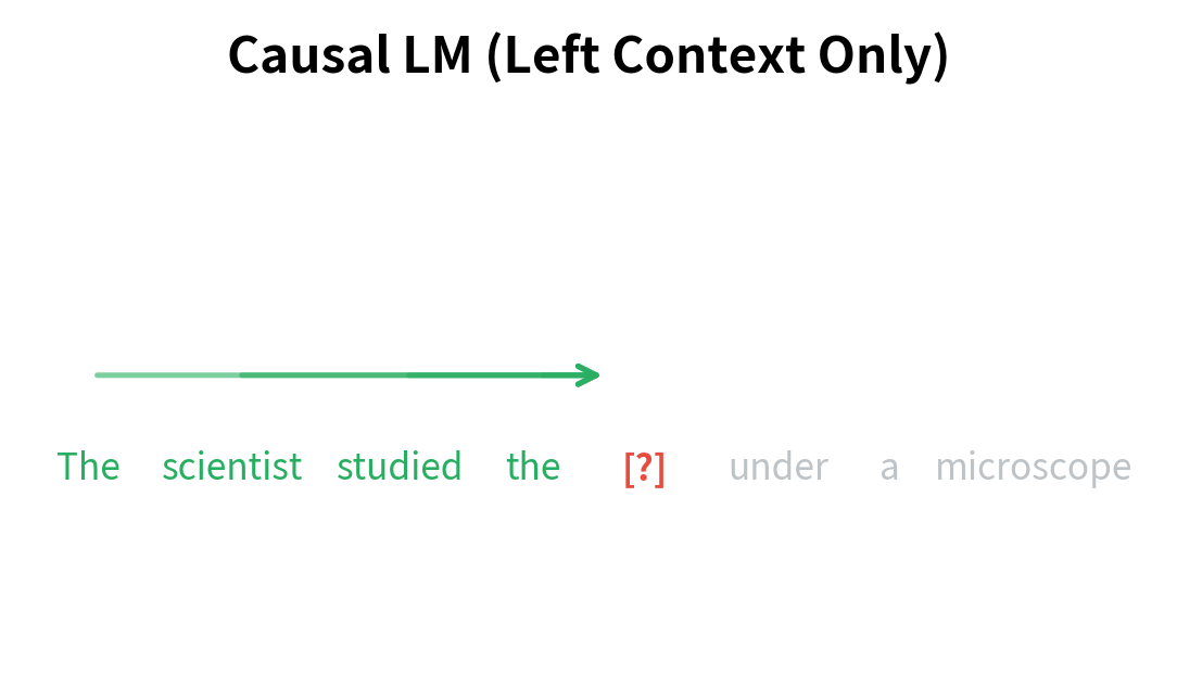
The core insight behind MLM is that understanding a word often requires seeing what comes after it, not just what came before. Consider the sentence:
The scientist studied the cell under a microscope.
When predicting "cell," a left-to-right model sees only "The scientist studied the." This provides some signal, but "cell" could still mean a prison cell, a biological cell, or a spreadsheet cell. The word "microscope" appearing later disambiguates completely, pointing to the biological meaning.
MLM allows the model to use this future context. By masking "cell" and asking the model to predict it, we force the model to integrate information from both "scientist studied" and "under a microscope" to make the prediction. The result is representations that encode richer semantic relationships.
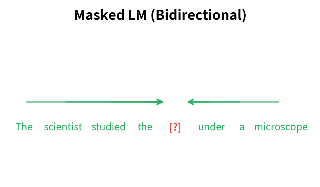
This bidirectional context is the key advantage of MLM. For classification, entailment, question answering, and other understanding tasks, seeing the full context produces better representations than the partial view available to autoregressive models.
The MLM Objective
How do we translate the intuition of "hide and predict" into a training objective? The answer involves three connected ideas: selecting which tokens to hide, defining what the model should predict, and measuring how well it succeeds. Let's build up the formalism step by step.
A pretraining objective where a fraction of input tokens are replaced with a special [MASK] token, and the model learns to predict the original tokens from the surrounding bidirectional context. Unlike causal LM, the model sees both left and right context when making predictions.
From Intuition to Formalism
Consider a sentence like "The cat sat on the mat." We want to train a model that can recover hidden words from context. The training procedure works as follows:
- Start with a complete sequence: We have , a sequence of tokens
- Select positions to mask: We randomly choose a subset of positions
- Corrupt the input: We create by replacing tokens at masked positions with
[MASK] - Predict the originals: The model must recover the original tokens at masked positions using the remaining context
The key insight is that step 4 requires the model to understand language deeply. To predict a masked word, the model must integrate syntactic constraints (what part of speech fits here?), semantic relationships (what meaning makes sense?), and world knowledge (what's plausible in this context?).
The Loss Function
We formalize "predict the originals" as maximizing the probability the model assigns to the correct tokens. Given the corrupted sequence , for each masked position , we want:
where is the probability the model with parameters assigns to the original token , conditioned on seeing the entire corrupted sequence . Note the conditioning: the model sees all of , including tokens both before and after position . This is the bidirectional context that distinguishes MLM from causal LM.
To combine predictions across all masked positions into a single training signal, we sum their log-probabilities:
where:
- : the masked language modeling loss we want to minimize
- : the set of masked position indices (typically , about 15% of positions)
- : the original token at position that we want to recover
- : the corrupted input sequence where tokens at positions in have been replaced
- : the probability the model assigns to the correct token, given bidirectional context
- : the log-probability, which is negative since probabilities lie in
Why Logarithms? Why Negative?
The formula uses logarithms for two reasons. First, products of probabilities become sums of log-probabilities, which are more numerically stable. Second, the logarithm creates a useful asymmetry in the loss signal.
When the model is confident and correct (), we have , contributing zero loss. When the model is uncertain (), we have , contributing moderate loss. When the model is wrong (), we have , contributing large loss.
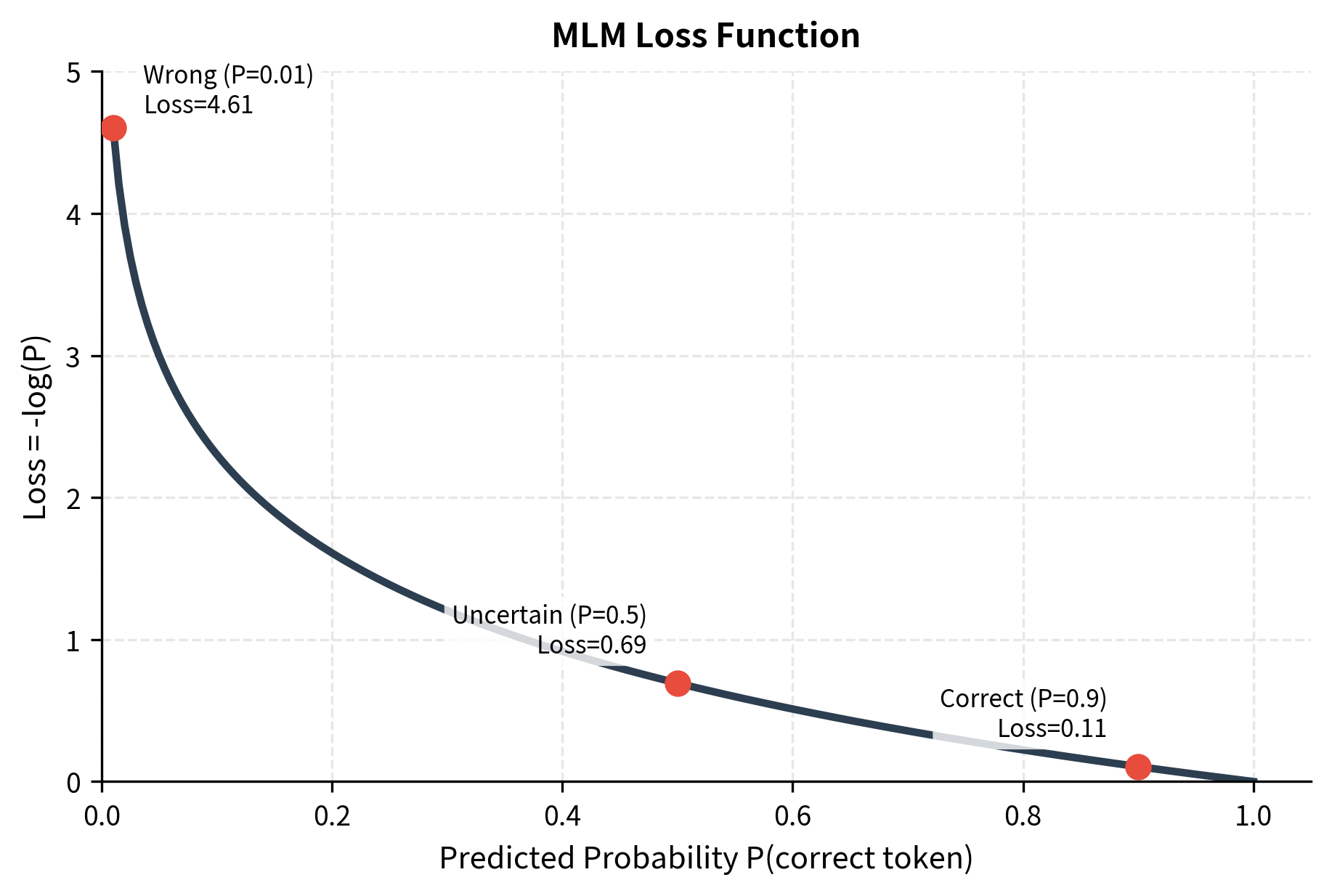
The negative sign in front of the sum flips these negative log-probabilities into positive loss values. Minimizing this loss pushes the model toward assigning high probability to the correct tokens.
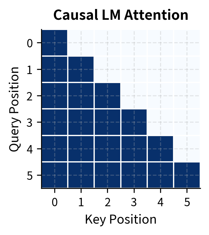
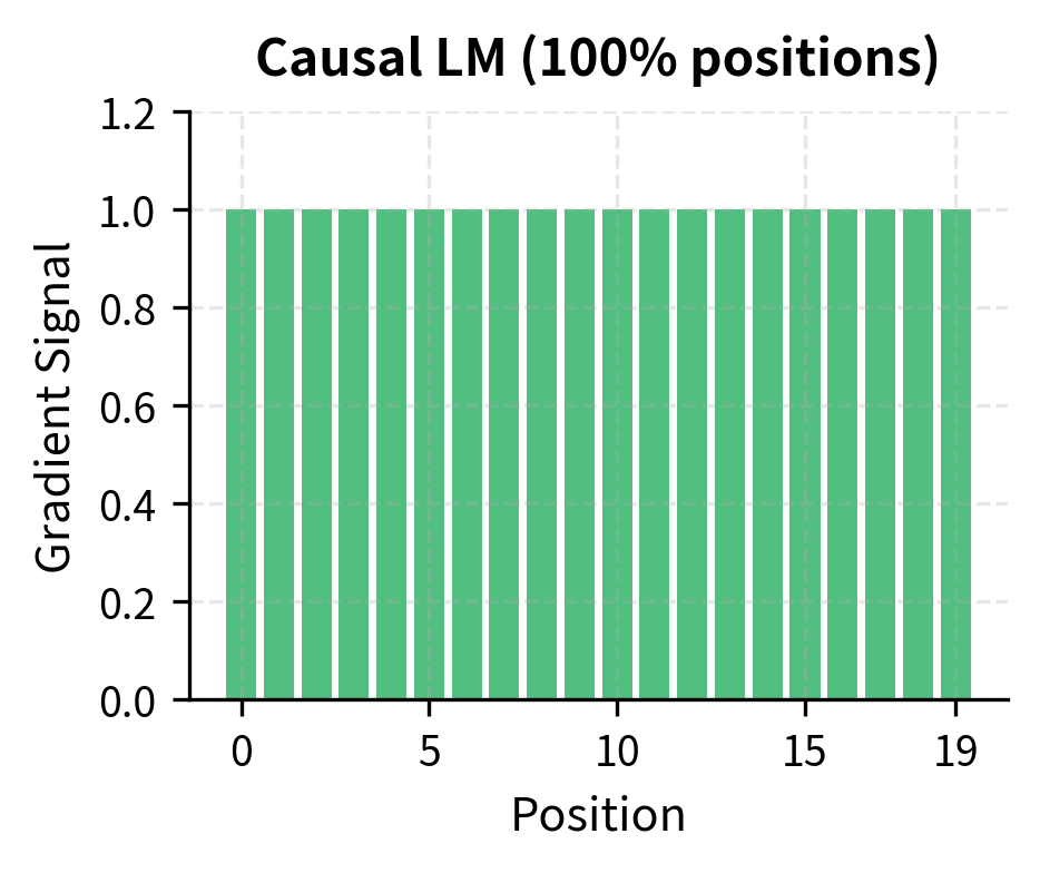
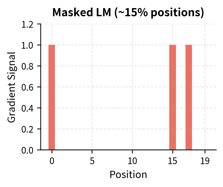
What Makes MLM Different from CLM
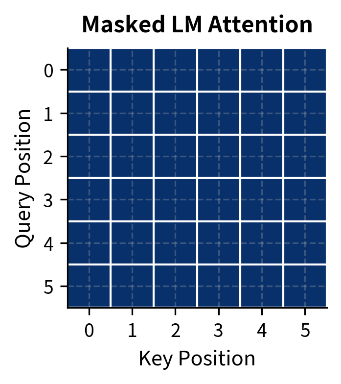
The summation in the MLM loss iterates only over masked positions , not all positions. This is fundamentally different from causal LM, where every position contributes to the loss. In CLM, predicting position 5 uses only positions 1-4. In MLM, predicting position 5 uses positions 1-4 and positions 6 onward, but only if position 5 is masked.
This trade-off has practical consequences: MLM is less sample-efficient per token (only 15% of positions contribute gradients), but each prediction benefits from richer context. The bidirectional signal compensates for the sparsity, producing representations that excel at understanding tasks.
The 15% Masking Rate
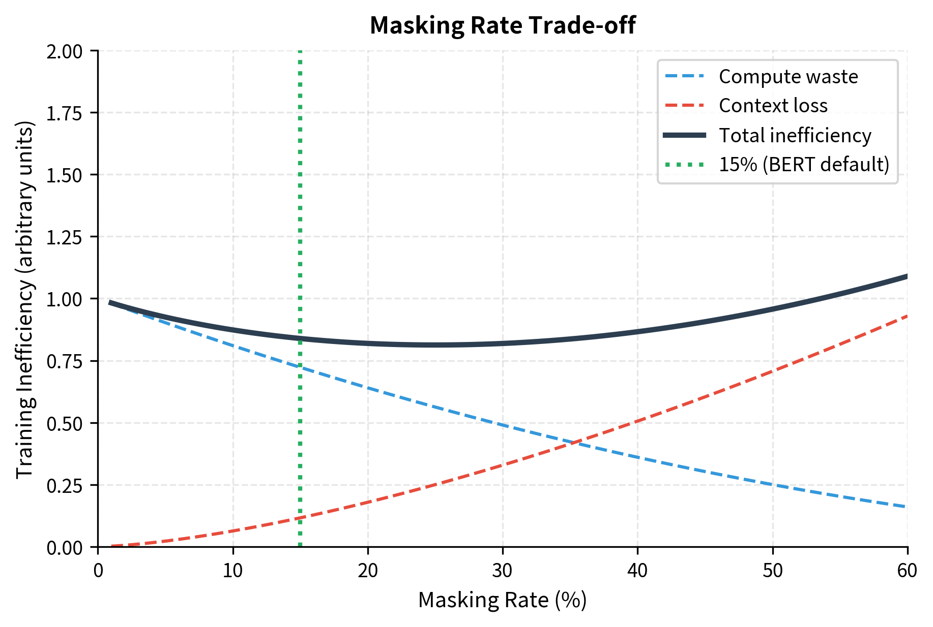
The original BERT paper established 15% as the masking rate: for each training example, approximately 15% of tokens are selected for prediction. This choice balances two competing concerns.
Masking too few tokens wastes compute. If only 1% of tokens are masked, 99% of the forward pass contributes nothing to the loss. The model processes the full sequence but learns from almost none of it.
Masking too many tokens destroys context. If 50% of tokens are masked, the model must predict half the sequence from the other half. With so much information missing, predictions become guesses rather than informed inferences.
The 15% rate emerged from empirical tuning. It provides enough masked tokens to learn efficiently while preserving enough context for accurate predictions. Later work has explored dynamic masking rates, but 15% remains the default for most MLM training.
The 80-10-10 Masking Strategy
Simply replacing all selected tokens with [MASK] creates a mismatch between training and inference. During training, the model sees [MASK] tokens everywhere. During fine-tuning and inference, it never sees them. This discrepancy can hurt transfer performance.
BERT addresses this with the 80-10-10 rule. For tokens selected for prediction:
- 80% are replaced with
[MASK] - 10% are replaced with a random token
- 10% are kept unchanged
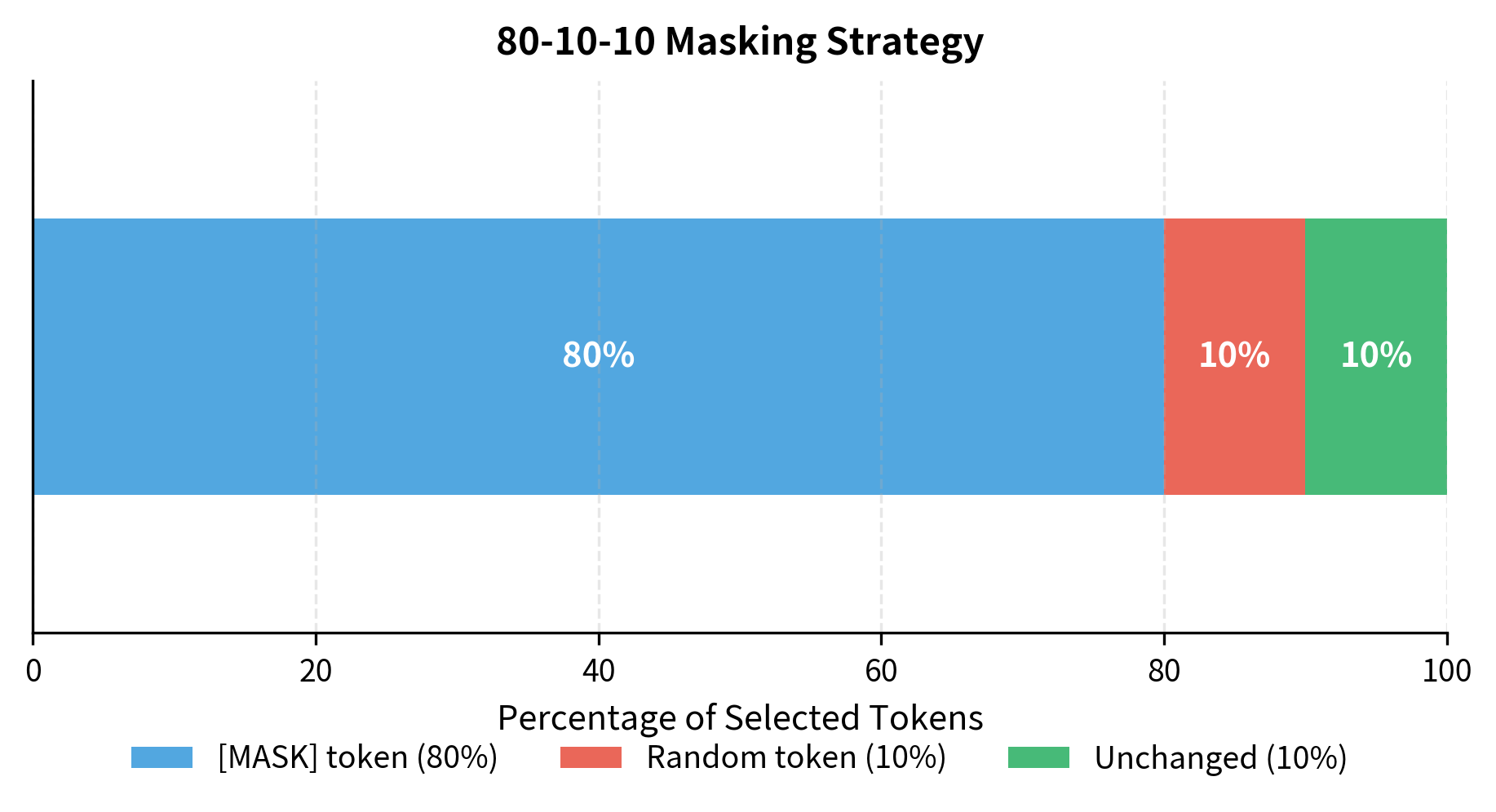
All three cases contribute to the loss: the model must predict the original token regardless of what replacement strategy was applied.
Let's see this masking function in action with a sample sequence:
The output shows how masking transforms the input. Positions where labels equals -100 are not masked and won't contribute to the loss. Positions with non-negative labels are masked positions where the model must predict the original token. Notice that some masked positions show the [MASK] token ID (103), while others show random tokens or remain unchanged, reflecting the 80-10-10 strategy.
The 80-10-10 strategy forces the model to:
- Learn to use context to recover masked tokens (the 80% case)
- Learn robust representations even when input contains noise (the 10% random case)
- Learn that unchanged tokens might still need prediction (the 10% unchanged case)
This last point is subtle but important. By sometimes requiring predictions on unchanged tokens, the model cannot simply "copy" visible tokens to the output. It must genuinely understand context, even for tokens that appear unmodified.
Understanding vs. Generation
MLM and CLM produce fundamentally different models suited for different tasks. The choice between them defines the model's capabilities.
Causal LM excels at generation because it models the natural process of producing text token by token. Each prediction extends the sequence, and the model can generate indefinitely by sampling from its predictions. GPT, LLaMA, and most chatbots use CLM.
Masked LM excels at understanding because it captures relationships in both directions. For classification, the model can integrate information from the entire input before making a decision. For question answering, it can match question words with answer words regardless of their positions. BERT, RoBERTa, and most embedding models use MLM.
Table mlm-vs-clm summarizes the key differences:
| Aspect | Causal LM | Masked LM |
|---|---|---|
| Context | Left only | Bidirectional |
| Primary use | Generation | Understanding |
| Loss positions | All positions | Masked only (~15%) |
| Inference | Autoregressive | Single pass |
| Example models | GPT, LLaMA | BERT, RoBERTa |
Neither approach is universally better. They're different tools optimized for different jobs. In practice, many systems combine both: an MLM encoder for understanding input, and a CLM decoder for generating output.
Implementing MLM Training
Let's implement a complete MLM training loop. We'll use a small transformer and train on sample text to see the dynamics in action.
With roughly 270,000 parameters, this is a tiny model by modern standards. BERT-base has 110 million parameters, and BERT-large has 340 million. Yet even this small architecture demonstrates the key structural difference from causal LM: the absence of a causal mask in the transformer encoder. Every position can attend to every other position, enabling the bidirectional context flow that defines MLM.
Now let's train on a simple corpus:
Our corpus contains 28 unique characters (26 letters plus space and newline), giving us a vocabulary of 29 after adding the [MASK] token. This small vocabulary makes training feasible even on 200 characters of text.
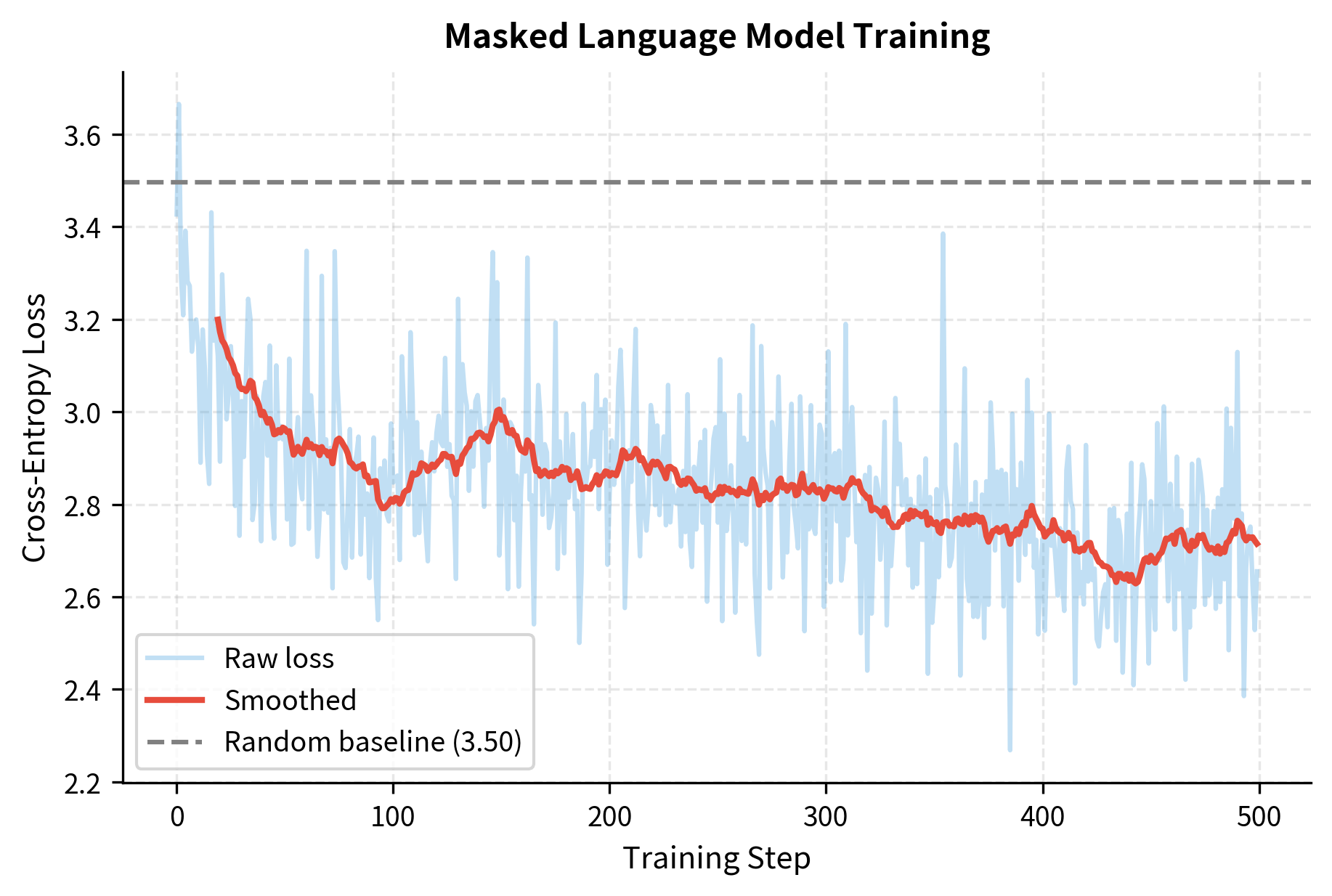
The loss dropped significantly from near the random baseline. A random model would assign equal probability to each token, yielding loss . Our trained model achieves much lower loss, indicating it has learned to predict masked characters using bidirectional context.
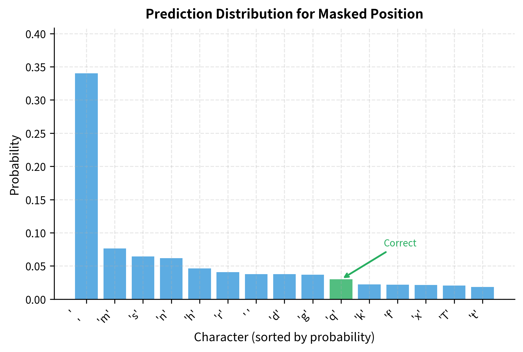
Let's see what the model predicts for masked tokens:
The model uses bidirectional context to inform its predictions. At position 4, it sees "The " before and "uick brown fox" after. At position 10, it sees "The quick " before and "rown fox" after. Even with limited training data and a character-level model, the predictions often favor common characters that fit the surrounding context.
MLM Training Dynamics
MLM training differs from CLM in several important ways that affect how models learn.
Sparse Gradients
Because only 15% of tokens are masked, only 15% of the output positions contribute to the gradient. This is less sample-efficient than CLM, where every position provides signal. To compensate, MLM models typically train for more steps or on more data.
No Exposure Bias
CLM suffers from "exposure bias": during training, the model always sees ground truth previous tokens, but during generation, it sees its own predictions. This mismatch can cause errors to compound.
MLM doesn't have this problem because it doesn't generate autoregressively. The model always conditions on the full (corrupted) input, both during training and inference. This makes MLM representations more robust for understanding tasks.
Independent Predictions
In MLM, predictions at different masked positions are made independently, in parallel. The model predicts all masked tokens simultaneously, not sequentially. This is efficient for training but means the model doesn't capture dependencies between masked tokens.
Consider masking both "New" and "York" in "I visited New York." CLM would predict "York" conditional on having already predicted "New." MLM predicts both independently, potentially outputting "New Orleans" and "Los Angeles" as individual predictions.
Dynamic Masking
The original BERT used static masking: each training example had the same tokens masked throughout training. RoBERTa introduced dynamic masking, where masking is applied fresh for each epoch.
With static masking, the same tokens are masked every time the model sees this sequence. With dynamic masking, different tokens are masked on each pass, exposing the model to more varied training signal from the same data. Dynamic masking provides more variety during training. The model sees the same underlying sequences but with different tokens masked, effectively multiplying the diversity of training signal. RoBERTa showed this simple change improves downstream performance, especially with longer training.
MLM for Representation Learning
The primary use of MLM is learning representations that transfer to downstream tasks. After pretraining, the model's hidden states capture rich semantic information that can be fine-tuned for classification, question answering, named entity recognition, and other tasks.
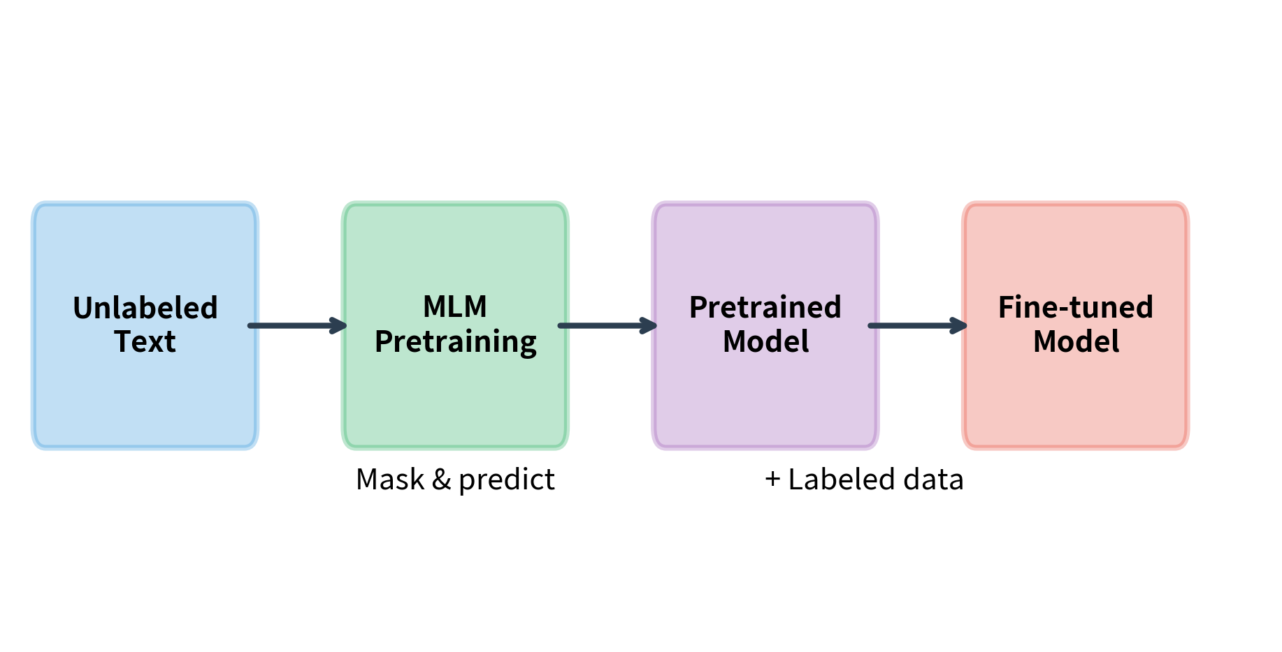
The typical workflow is:
- Pretrain on large unlabeled corpus with MLM objective
- Fine-tune on labeled data for specific task
- Infer using the fine-tuned model
During fine-tuning, the [MASK] token is never used. The model processes normal text and uses its pretrained representations as a starting point. Fine-tuning updates all weights to adapt to the specific task.
Limitations and Impact
Masked language modeling has transformed NLP, but it comes with fundamental limitations that shape its applications.
The inability to generate text is the most significant constraint. MLM models cannot produce coherent sequences token by token. They can fill in blanks and score existing text, but they cannot write. This limitation means MLM is unsuitable for chatbots, story generation, code completion, and other generative applications. The distinction between understanding and generation has driven the field toward hybrid architectures that combine MLM-style encoders with CLM-style decoders, as seen in T5 and BART.
The masking mismatch between pretraining and fine-tuning creates subtle issues. During pretraining, 15% of tokens are corrupted. During fine-tuning, no tokens are masked. The 80-10-10 strategy mitigates this by keeping some tokens unchanged, but the model still never sees the [MASK] token after pretraining. Research on continuous masking and better pretraining objectives continues to address this gap.
Sample efficiency is another concern. With only 15% of tokens contributing to the loss, MLM requires more compute than CLM to see the same amount of training signal. RoBERTa compensated by training longer and on more data, but this increases cost. Recent work on efficient pretraining explores higher masking rates and alternative objectives.
Despite these limitations, MLM unlocked capabilities that seemed impossible before. BERT's bidirectional representations set new state-of-the-art results on eleven NLP benchmarks when released. The pretrain-then-fine-tune paradigm it established remains the dominant approach for understanding tasks. Sentence embeddings from MLM models power semantic search, document clustering, and similarity computations across the industry. The insight that bidirectional context improves understanding has influenced the design of virtually every model since.
Key Parameters
When training MLM models, several parameters significantly impact performance:
- mask_prob (default: 0.15): Fraction of tokens to mask per sequence. Higher values provide more training signal but destroy more context. The 15% rate from BERT remains standard, though some work explores 40% or higher with adjusted strategies.
- d_model: Hidden dimension of the transformer. BERT-base uses 768, BERT-large uses 1024. Larger values increase model capacity but require proportionally more compute and memory.
- n_heads: Number of attention heads. Should divide d_model evenly. BERT-base uses 12 heads (64 dimensions each), BERT-large uses 16 heads.
- n_layers: Number of transformer layers. BERT-base uses 12, BERT-large uses 24. Deeper models capture more complex patterns but are slower to train and infer.
- max_len: Maximum sequence length the model can process. BERT uses 512 tokens. Longer contexts require quadratically more memory for attention but capture more context.
- learning_rate: Typically 1e-4 to 5e-4 for MLM pretraining. BERT used 1e-4 with warmup. Higher rates speed training but risk instability.
- batch_size: Larger batches provide more stable gradients. BERT used effective batch sizes of 256 sequences. MLM benefits from large batches since only 15% of tokens contribute to each gradient.
Summary
Masked language modeling trains models to predict randomly masked tokens from bidirectional context. This chapter covered the key concepts:
- Bidirectional context allows MLM models to use information from both before and after each position, producing richer representations than unidirectional models
- The 15% masking rate balances sample efficiency against context preservation, providing enough training signal while keeping most context visible
- The 80-10-10 strategy (80%
[MASK], 10% random, 10% unchanged) reduces the mismatch between pretraining and fine-tuning - MLM vs. CLM represents a fundamental trade-off: MLM excels at understanding tasks while CLM excels at generation
- Dynamic masking applies fresh masks each epoch, increasing training signal diversity
- Sparse gradients from masking only 15% of positions make MLM less sample-efficient than CLM
The next chapter explores whole word masking, a refinement that improves MLM by masking entire words rather than individual subword tokens.
Quiz
Ready to test your understanding? Take this quick quiz to reinforce what you've learned about masked language modeling.

Comments