

Learn how ALiBi encodes position through linear attention biases instead of embeddings. Master head-specific slopes, extrapolation properties, and when to choose ALiBi over RoPE for length generalization.

This article is part of the free-to-read Language AI Handbook
Choose your expertise level to adjust how many terms are explained. Beginners see more tooltips, experts see fewer to maintain reading flow. Hover over underlined terms for instant definitions.
ALiBi: Attention with Linear Biases
In the previous chapters, we explored various approaches to encoding position information: sinusoidal encodings that add fixed patterns to embeddings, learned position embeddings that train position vectors from scratch, relative position encodings that capture pairwise distances, and RoPE that rotates embeddings based on position. Each method has trade-offs involving complexity, performance, and the ability to handle sequences longer than those seen during training.
ALiBi (Attention with Linear Biases) takes a radically different approach. Instead of modifying embeddings or inventing clever rotation schemes, ALiBi simply subtracts a value from attention scores based on the distance between tokens. The farther apart two tokens are, the larger the penalty. This remarkably simple idea, introduced by Press et al. in 2022, achieves strong performance while enabling something the other methods struggle with: extrapolation to sequences far longer than anything seen during training.
The Extrapolation Problem
Before understanding ALiBi's solution, we need to appreciate the problem it solves. Transformers trained on sequences of length often fail dramatically when given sequences of length or beyond. The sinusoidal encodings produce positions the model has never seen. Learned position embeddings simply don't exist for positions beyond the training range. Even RoPE, despite its theoretical elegance, can struggle with extreme extrapolation.
Length extrapolation refers to a model's ability to process sequences longer than those encountered during training while maintaining reasonable performance. Many position encoding schemes fail this test because they produce position representations the model has never learned to interpret.
Why does this matter? Training on very long sequences is computationally expensive due to attention's quadratic complexity. If we could train on shorter sequences and deploy on longer ones, we'd save enormous resources. More practically, real-world applications often encounter documents, conversations, or code files that exceed training lengths. A model that degrades gracefully on longer inputs is far more useful than one that fails catastrophically.
The Core Idea: Penalizing Distance
ALiBi's insight is elegant in its simplicity: don't encode position in the embeddings at all. Instead, modify the attention mechanism itself to prefer nearby tokens over distant ones.
Consider what attention scores represent: they measure compatibility between a query and a key. After softmax, these scores determine how much each position contributes to the output. ALiBi introduces a simple bias that subtracts from the score based on distance:
where:
- : the modified attention score between positions and
- : the original dot product between query and key
- : a slope parameter that controls how aggressively to penalize distance
- : the absolute distance between the two positions
The subtraction means distant tokens receive lower scores. A token 10 positions away gets penalized by , while an adjacent token gets penalized by just . After softmax normalization, this translates to nearby tokens receiving higher attention weights.
ALiBi adds a linear bias to attention scores based on the distance between query and key positions. The bias is always negative, penalizing distant positions. The penalty grows linearly with distance, controlled by a slope parameter .
This is position encoding without position embeddings. The model learns nothing about position during pretraining of the embeddings themselves. Position information enters only through the attention bias, and only at the moment of computing attention scores.
The Mathematical Formulation
Now that we understand ALiBi's core insight, let's develop the complete mathematical framework. We'll build from standard attention to ALiBi-augmented attention, showing exactly where and how the position bias enters the computation.
Starting Point: Standard Scaled Dot-Product Attention
Recall that standard self-attention operates on three matrices derived from the input sequence. For a sequence of tokens:
where:
- : the query matrix containing query vectors for all positions
- : the key matrix containing key vectors for all positions
- : the value matrix containing value vectors for all positions
- : the dimension of queries and keys
- : the raw attention score matrix where entry is the dot product between query and key
- : scaling factor that prevents dot products from growing too large in high dimensions
The matrix captures content-based similarity: how much each query "wants" to attend to each key based purely on their learned representations. But this matrix is blind to position. Token 1 attending to token 2 produces the same score whether they're adjacent or separated by 500 tokens. This is where ALiBi intervenes.
Injecting Position: The Bias Matrix
ALiBi's modification is surgical. Rather than changing how queries, keys, or values are computed, it adds a single term to the attention scores:
The bias matrix is added directly to the scaled scores before softmax. This is the only change to standard attention. The matrix encodes position information through a remarkably simple rule:
where:
- : the bias added to the attention score between query position and key position
- : the slope parameter for this attention head (controls penalty strength)
- : the absolute distance between positions and
Let's unpack why this formula works. The absolute distance measures how far apart two positions are in the sequence. Adjacent tokens have distance 1, tokens separated by 10 positions have distance 10. Multiplying by a positive slope and negating creates a penalty that grows linearly with distance.
Consider what happens for a query at position 5 attending to various keys:
- Attending to position 5 (itself): (no penalty)
- Attending to position 4 (adjacent): (small penalty)
- Attending to position 0 (distant): (large penalty)
The negative bias reduces the attention score, and larger distances produce more negative biases. After softmax normalization, this translates to lower attention weights for distant tokens. The content-based similarity in still matters, but now it competes against a distance penalty.
The Causal Case: Masking the Future
For decoder-style models that generate text left-to-right, we need causal masking: position can only attend to positions . The combined bias matrix looks like:
The structure reveals two distinct components:
-
Lower triangle (including diagonal): Contains the ALiBi distance penalties. The diagonal is 0 (self-attention has no penalty), and values increase as you move left (farther from the query position).
-
Upper triangle: Contains values from the causal mask. These become 0 after softmax, preventing any attention to future positions.
The entries ensure that after , future positions contribute nothing to the weighted sum. The linear penalties in the lower triangle shape how attention flows among the allowed past positions.
Building the Bias Matrix: Step-by-Step Implementation
Let's translate this mathematics into code, building up the bias matrix piece by piece.
The key insight is using NumPy broadcasting to compute all pairwise distances at once. By reshaping the position array into a column vector positions[:, None] and a row vector positions[None, :], subtraction produces an matrix where entry is . Taking the absolute value gives us the distance matrix.
Let's see what this produces for a small sequence:
Reading this matrix: the diagonal is zero because a token attending to itself has distance zero. Moving away from the diagonal in either direction, penalties grow linearly. Position 5 (row 5) attending to position 0 (column 0) shows , exactly as expected. The matrix is symmetric because distance is symmetric: .
For decoder models, we overlay the causal mask:
The np.triu function creates an upper triangular matrix of ones, which we use to identify positions that should be masked. The k=1 argument excludes the diagonal, since a token should be able to attend to itself.
Now the upper triangle shows inf (NumPy's display for ), while the lower triangle retains the distance penalties. Row 5 can attend to all previous positions with penalties for positions 0 through 5 respectively. Row 0 can only attend to itself with penalty 0.
Let's visualize both the distance matrix and the resulting causal ALiBi bias matrix side by side:
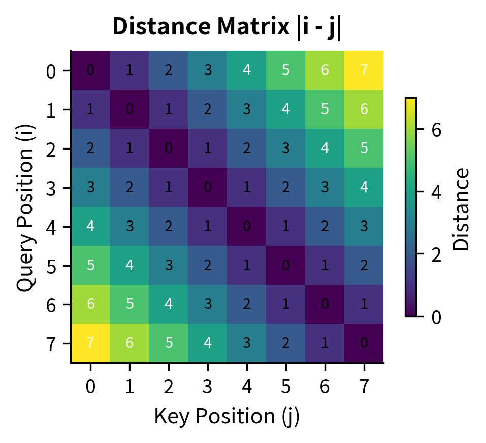
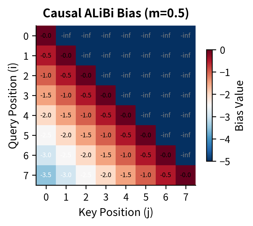
The left matrix shows raw distances: the diagonal is 0 (same position), adjacent cells are 1, and values grow as positions diverge. The right matrix shows what happens after applying ALiBi: distances become negative penalties (scaled by the slope), and the upper triangle is masked to enforce causality.
Head-Specific Slopes
ALiBi uses different slope values for different attention heads. This is crucial: a single slope would force all heads to have the same locality preference, but different heads benefit from different perspectives. Some heads might focus on very local context (steep slope, harsh penalties for distance), while others maintain broader receptive fields (gentle slope, mild penalties).
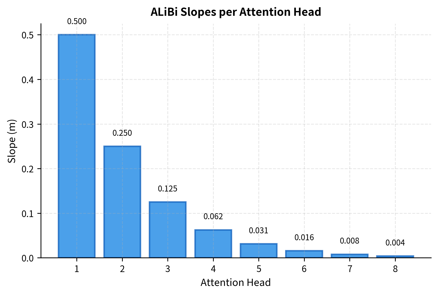
The slopes are not learned but fixed according to a geometric sequence. For a model with attention heads, the slope for head is:
where:
- : the slope parameter for attention head
- : the total number of attention heads in the model
- : the head index, ranging from 1 to
- : a scaling factor that ensures slopes span a consistent range regardless of head count
- : the denominator that grows exponentially with head index
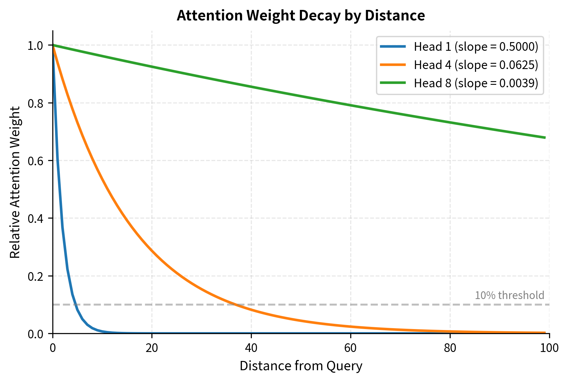
The base of 8 in the exponent was chosen empirically by the ALiBi authors. It ensures that slopes span roughly 8 orders of magnitude when divided across the heads. With 8 heads, the exponent simplifies to just , giving slopes of , which equals .
The geometric progression ensures that slopes span several orders of magnitude. With 8 heads, the steepest slope (0.5) penalizes a distance of 10 by 5 logits, effectively eliminating distant tokens from consideration. The gentlest slope (roughly 0.004) penalizes the same distance by only 0.04 logits, allowing the head to attend broadly.
Visualizing the Attention Bias
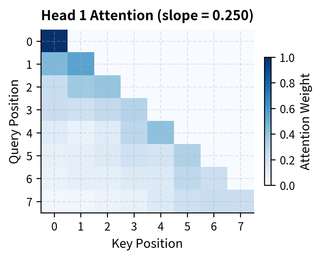
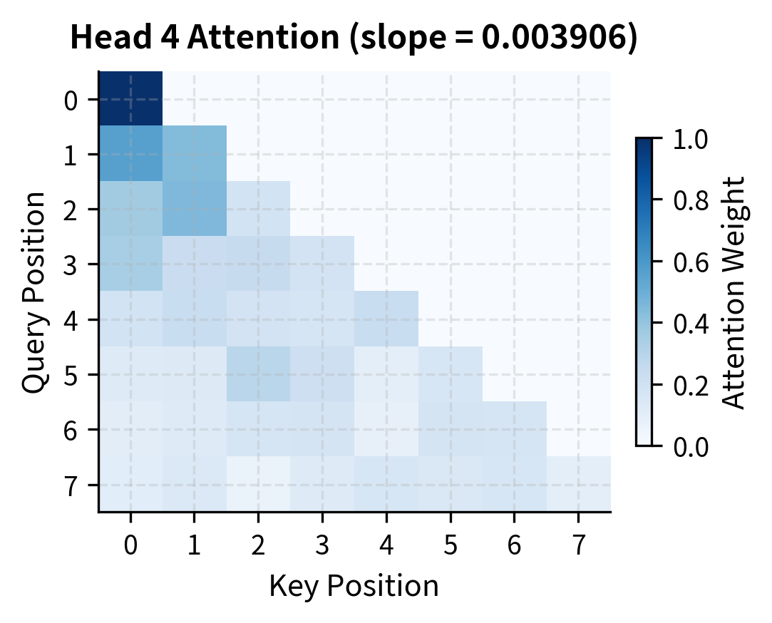
Let's visualize how ALiBi biases affect attention patterns for different heads:
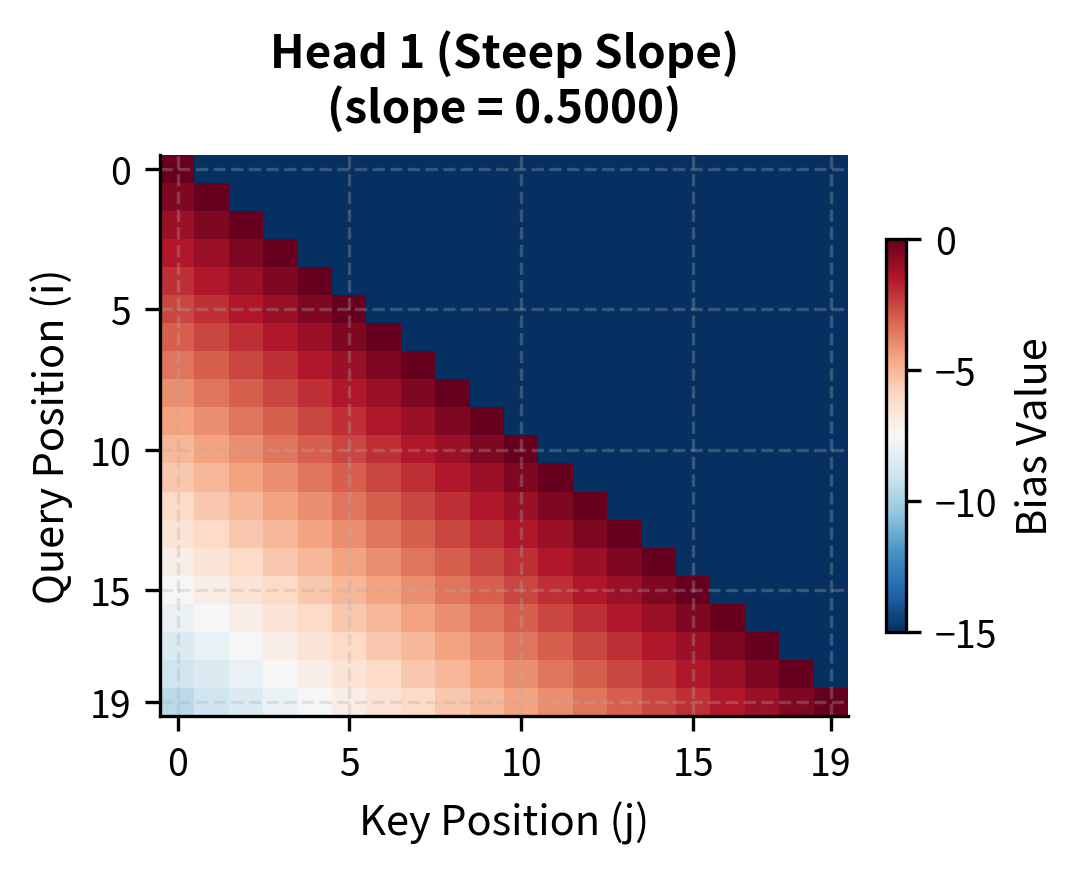
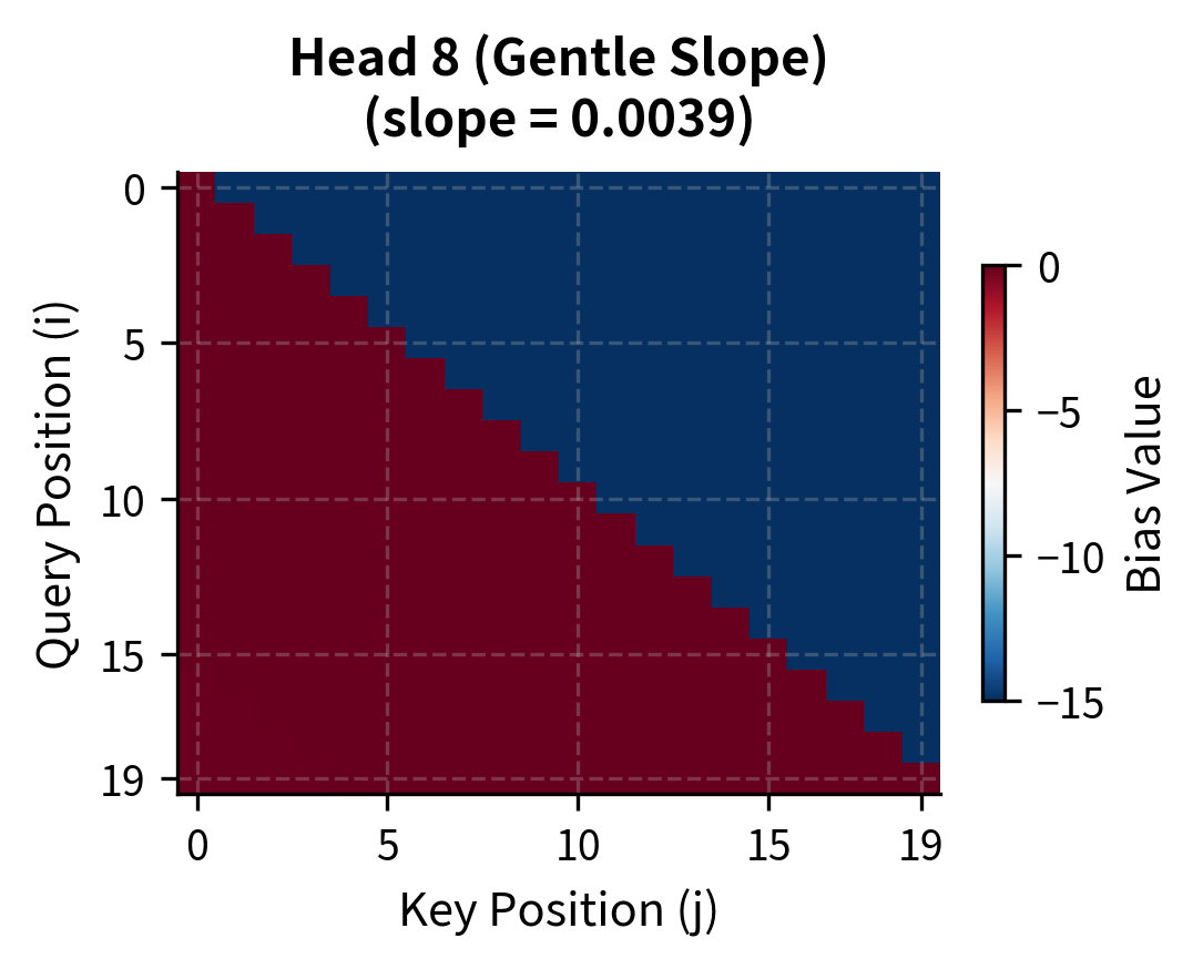
The contrast is stark. Head 1's bias matrix shows deep blue (strongly negative) values just a few positions from the diagonal. By position 10, the penalty exceeds -5 logits, making those tokens nearly invisible after softmax. Head 8, in contrast, shows mild penalties throughout. Even at distance 19, the penalty is less than 0.1 logits, allowing meaningful attention to distant tokens.
This division of labor is intentional. Linguistic phenomena operate at different scales: adjacent tokens matter for syntax and local coherence, while distant tokens matter for coreference, topic consistency, and long-range dependencies. By giving different heads different locality preferences, ALiBi enables the model to capture phenomena at multiple scales simultaneously.
ALiBi in Attention: Complete Implementation
Now let's implement ALiBi-augmented attention from scratch:
Let's test this implementation with a simple example:
Compare the attention patterns between heads. Head 1 with its steep slope concentrates attention heavily on recent positions, with weights dropping rapidly as distance increases. Head 4 with its gentle slope distributes attention more evenly across the available context.
To understand the impact of ALiBi more directly, let's compare attention patterns with and without the position bias. We'll compute attention for the same queries and keys, once with standard attention (no position encoding) and once with ALiBi:
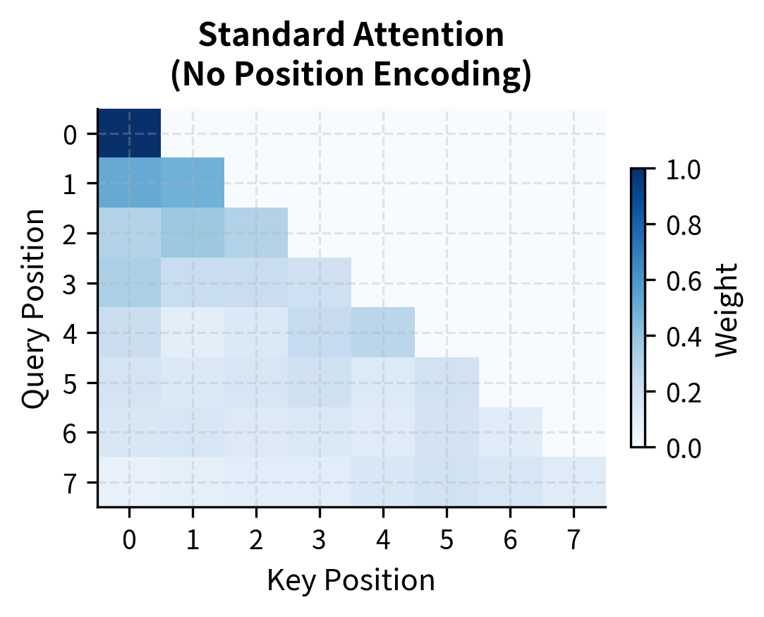
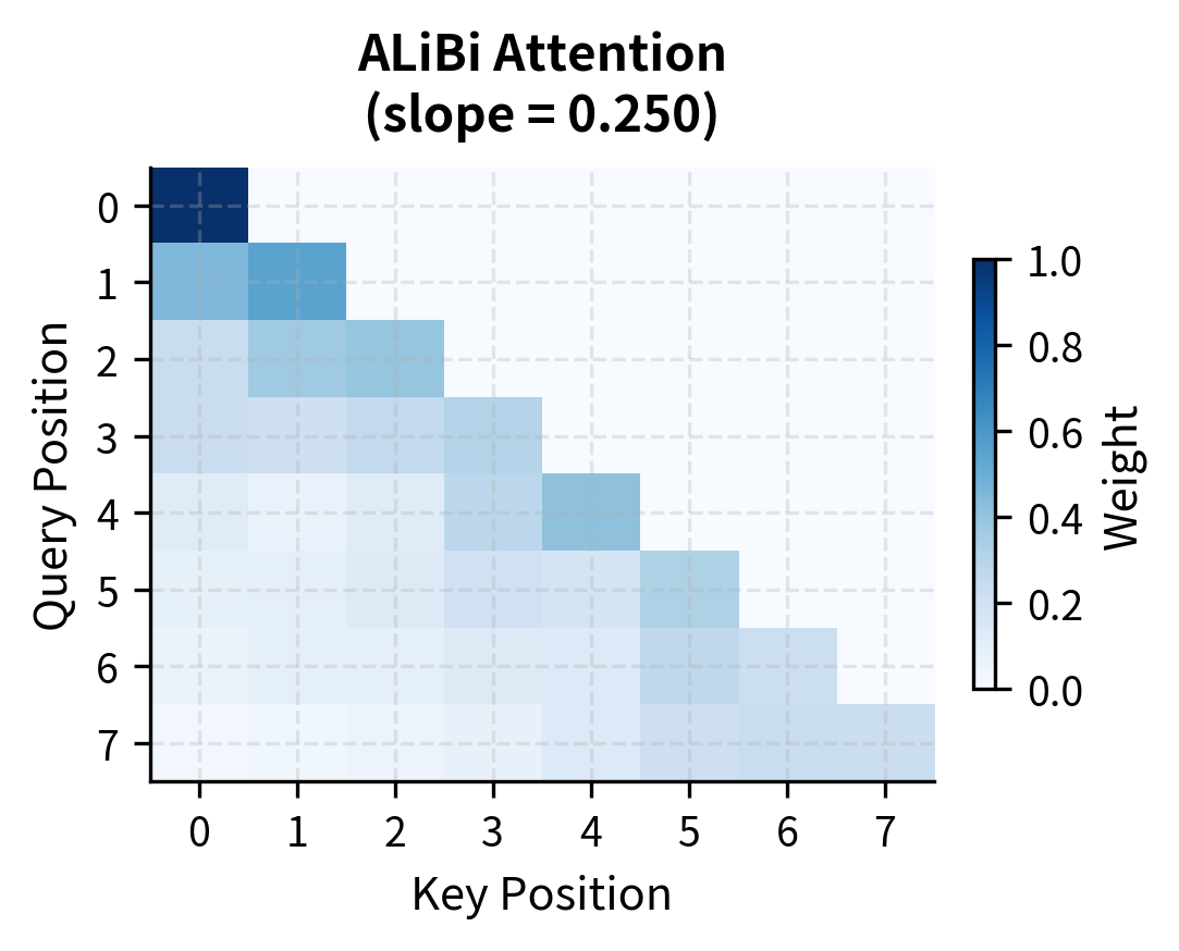
The difference is striking. Standard attention distributes weight based purely on content similarity, sometimes attending strongly to distant positions. ALiBi reshapes this pattern, pulling attention toward recent tokens while still allowing content to influence the final distribution. This locality bias emerges from a single matrix addition, requiring no learned position embeddings.
Why ALiBi Extrapolates
The key to ALiBi's extrapolation ability lies in what the model learns during training. With other position encoding schemes, the model learns to interpret specific position representations. A sinusoidal encoding for position 512 produces a particular pattern that the model has seen and learned to use. A learned position embedding for position 512 is a specific trained vector. When you encounter position 513 or 1024, these are novel representations the model hasn't seen.
ALiBi sidesteps this problem entirely. The model never learns position representations because there are none. Instead, it learns to work with relative attention patterns shaped by the linear bias. During training on sequences of length 1024, the model sees attention patterns where nearby tokens are favored and distant tokens are penalized. This is true at position 10, position 500, and position 1000.
When inference extends to position 2048, the same principle applies. The local neighborhood still receives favorable bias. Tokens 10 positions away still get penalized by the same amount. The absolute positions are larger, but the relative structure is unchanged. The model has learned to extract information from attention patterns that favor locality, and those patterns remain consistent regardless of sequence length.
ALiBi extrapolates because it encodes relative distance, not absolute position. The linear penalty for distance 10 is the same whether you're at position 50 or position 5000. The model learns to work with distance-biased attention patterns, which remain consistent across sequence lengths.
Let's visualize this consistency:
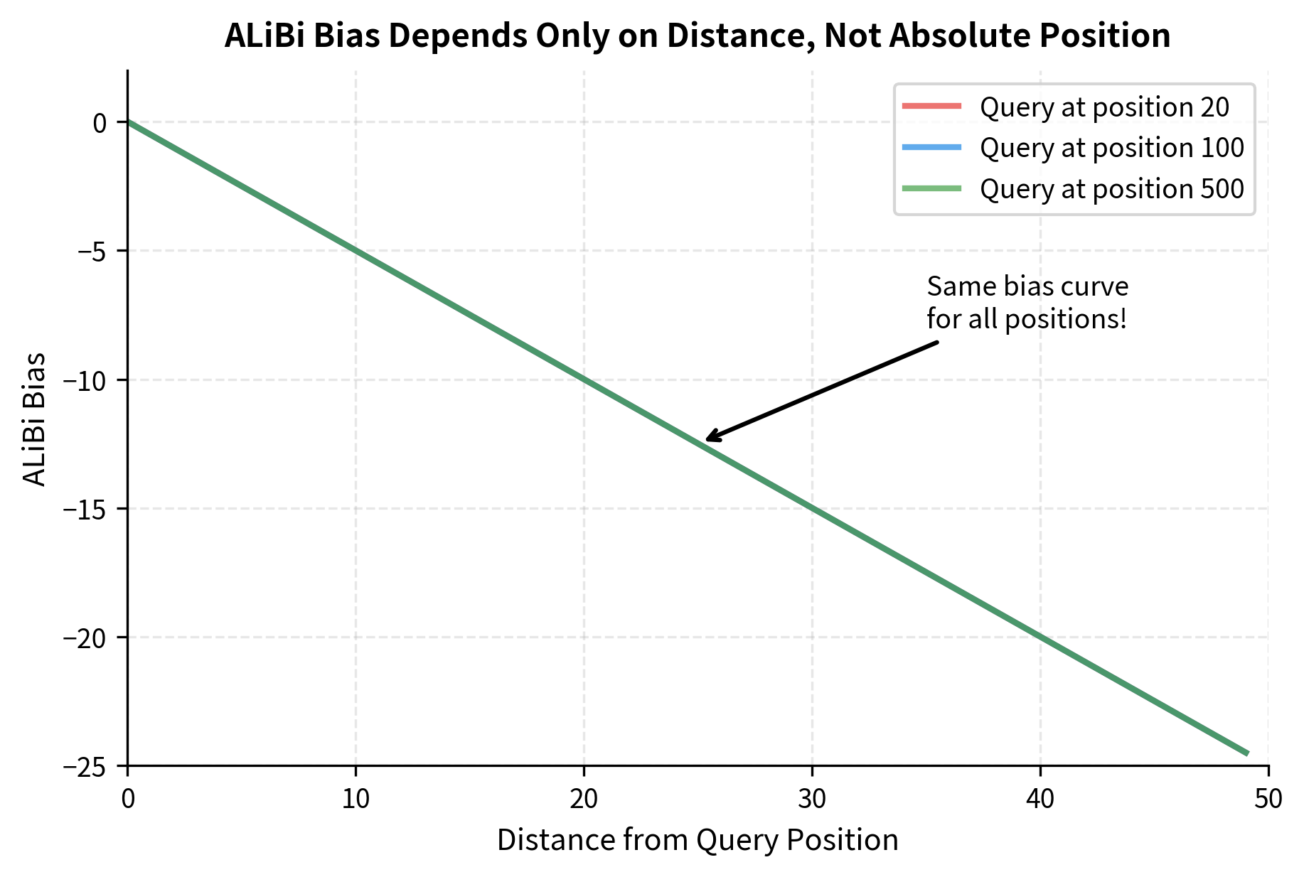
The curves overlap perfectly because ALiBi's bias depends only on distance, never on absolute position. This is the mathematical basis for length extrapolation.
ALiBi vs RoPE: A Comparison
Both ALiBi and RoPE are widely used in modern language models, and both handle relative position. But they take fundamentally different approaches:
| Aspect | ALiBi | RoPE |
|---|---|---|
| Position encoding location | Attention bias | Query/key embeddings |
| Mechanism | Subtracts linear penalty from scores | Rotates Q and K vectors |
| Parameters | Fixed slopes (no training) | No additional parameters |
| Computation | Simple matrix addition | Complex number arithmetic or rotation matrices |
| Extrapolation | Strong out-of-the-box | Requires additional techniques (e.g., scaling) |
| Relative position | Implicit through distance penalty | Explicit through rotation angle differences |
RoPE encodes position by rotating query and key vectors. When computing dot products, the rotation angles combine such that the result depends on relative position. This is elegant and theoretically motivated, but the rotation patterns at unseen positions can behave unexpectedly.
ALiBi's approach is more brutalist: just penalize distance. There's no rotation, no complex number interpretation, no interplay between embedding dimensions. The simplicity has practical benefits. ALiBi requires no changes to the embedding pipeline and adds minimal computational overhead.
Let's compare implementation complexity:
The ALiBi bias is a single line of code added to standard attention. RoPE requires restructuring how queries and keys are computed. Both work, but ALiBi's simplicity is a genuine advantage for implementation and debugging.
Practical Considerations
When should you choose ALiBi? Consider these factors:
Training efficiency. ALiBi adds minimal overhead. The bias computation is a simple matrix operation that's negligible compared to the attention computation itself. There are no additional parameters to train.
Length flexibility. If your deployment might encounter sequences longer than training, ALiBi provides a safety net. Models like BLOOM and MPT use ALiBi partly for this reason.
Simplicity. ALiBi is easy to implement correctly. The fixed slopes mean no hyperparameter tuning for the position encoding itself. Debugging attention patterns is straightforward because the bias is directly interpretable.
Limitations. ALiBi's linear penalty may not capture all positional relationships. Some tasks might benefit from RoPE's more nuanced encoding. Extremely local heads (with steep slopes) can struggle if a task genuinely requires attending to distant tokens with equal strength.
In practice, many production models use either ALiBi or RoPE, with the choice often depending on the team's preferences and empirical results on target tasks. Both represent significant advances over sinusoidal encodings and learned position embeddings.
Limitations and Impact
ALiBi's simplicity is both its strength and its limitation. The linear penalty assumes that relevance decreases monotonically with distance, which is generally true for language but not universally. Some linguistic phenomena, like matching parentheses in code or tracking long-distance agreement in legal documents, might benefit from attention patterns that don't decay linearly.
The fixed slopes, while eliminating hyperparameters, also remove flexibility. A model cannot learn task-specific locality preferences through the position encoding itself. If a particular downstream task requires unusual attention patterns, the model must learn to overcome the ALiBi bias through the content-based attention scores.
Despite these limitations, ALiBi has proven remarkably effective. The BLOOM family of models, including the 176-billion parameter BLOOM-176B, uses ALiBi. So does MPT (MosaicML Pretrained Transformer). These models demonstrate that ALiBi scales to the largest models and handles diverse tasks well.
The impact of ALiBi extends beyond its direct use. It demonstrated that position encoding can be far simpler than previously thought. The original Transformer's sinusoidal encodings were ingenious but perhaps overengineered for the task. ALiBi showed that a linear penalty on distance, applied at attention time, is sufficient for strong performance. This insight has influenced subsequent work on efficient transformers and position encoding schemes.
Key Parameters
When implementing ALiBi in your own models, these parameters determine behavior:
-
num_heads: The number of attention heads in your model. ALiBi automatically computes slopes for each head using the geometric sequence formula. More heads create finer granularity in locality preferences. -
slope(m): The penalty strength for each head. Steeper slopes (larger values like 0.5) create strong locality bias where attention concentrates on nearby tokens. Gentler slopes (smaller values like 0.004) allow broader attention across the sequence. These are fixed by the formula, not tuned. -
causal: Whether to apply causal masking. Set toTruefor decoder-style autoregressive models where tokens can only attend to previous positions. Set toFalsefor encoder-style bidirectional attention. -
Base value (8): The constant in the slope formula that controls the range of slopes. The original ALiBi paper uses 8, which ensures slopes span several orders of magnitude. This value is typically not modified.
Summary
ALiBi offers a refreshingly simple approach to position encoding:
-
No position embeddings. Position enters only through attention biases, not through modifications to token representations.
-
Linear distance penalty. Attention scores are reduced by , where is a head-specific slope and is the distance between query position and key position . Nearby tokens are favored, distant tokens are penalized.
-
Geometric slopes. Different attention heads use different slopes, creating multi-scale attention. Some heads focus locally, others attend broadly.
-
Strong extrapolation. Because only relative distance matters (not absolute position), models trained on short sequences can process longer sequences at inference time.
-
Minimal overhead. ALiBi adds one matrix addition to attention computation. No additional parameters, no complex rotation arithmetic.
The next chapter will compare all position encoding methods we've covered: sinusoidal, learned, relative, RoPE, and ALiBi. You'll see how each handles key challenges like extrapolation, computational cost, and representational power.
Quiz
Ready to test your understanding? Take this quick quiz to reinforce what you've learned about ALiBi (Attention with Linear Biases).

Comments