

Master decoder-only transformers powering GPT, Llama, and modern LLMs. Learn causal masking, autoregressive generation, KV caching, and GPT-style architecture from scratch.

This article is part of the free-to-read Language AI Handbook
Choose your expertise level to adjust how many terms are explained. Beginners see more tooltips, experts see fewer to maintain reading flow. Hover over underlined terms for instant definitions.
Decoder Architecture
The transformer decoder is the engine behind text generation. While encoders excel at understanding input sequences, decoders specialize in producing sequences, one token at a time. Every time you interact with ChatGPT, Claude, or Llama, you're witnessing a decoder at work: taking your prompt and generating a coherent response by predicting one token after another.
What makes the decoder special is its causal nature. Unlike encoders that can look at the entire input simultaneously, decoders must respect temporal order. When generating the fourth word, the model can only consider words one through three. It cannot peek ahead at words five or six because those don't exist yet. This constraint, enforced through causal masking, defines the decoder's fundamental architecture.
In this chapter, we'll explore the decoder-only design that powers modern language models like GPT, the mechanism of causal masking that enforces left-to-right generation, and how multiple decoder layers stack to create increasingly sophisticated language understanding.
The Decoder-Only Design
The original transformer from "Attention Is All You Need" (2017) used both an encoder and a decoder for machine translation. But a pivotal discovery emerged: for language modeling, you don't need the encoder at all. A stack of decoder blocks, trained to predict the next token, learns rich representations of language without any encoder component.
A decoder-only model consists of a stack of transformer blocks that process tokens autoregressively. Each block uses causal (masked) self-attention to ensure that predictions at position depend only on positions .
The decoder-only approach offers several advantages:
- Simplicity: One stack of layers instead of two (no encoder-decoder attention needed)
- Unified architecture: The same model handles both understanding and generation
- Scalability: Easier to scale parameters when you have a single stack
- Pretraining efficiency: Next-token prediction provides dense supervision at every position
GPT-1, GPT-2, GPT-3, and their successors all use this decoder-only design. So do Llama, Mistral, and most open-source language models. The architecture has become the default choice for generative language AI.
Understanding Autoregressive Generation
Before diving into the architecture, let's clarify what autoregressive generation means in practice. The decoder generates text one token at a time, where each new token is conditioned on all previously generated tokens.
Given a prompt "The cat sat on the", generation proceeds as follows:
- Process the prompt through the decoder to get a representation for each position
- Use the representation at the final position to predict the next token: "mat"
- Append "mat" to the sequence and process again
- Use the new final position to predict the next token: "and"
- Continue until generating a stop token or reaching a length limit
Mathematically, we're factorizing the joint probability of a sequence into a product of conditional probabilities. This is known as the chain rule of probability, and it expresses the idea that generating a sequence is equivalent to making a series of next-token predictions:
where:
- : the joint probability of the entire sequence of tokens
- : the token at position in the sequence
- : the total sequence length
- : the product over all positions from 1 to
- : the conditional probability of token given all previous tokens
Each factor in this product represents one prediction step. The factor predicts the first token with no context. The factor predicts the second token given the first. By the time we reach , we're predicting the final token given the entire preceding context.
The decoder computes each of these conditional probabilities. It takes the sequence so far, applies its transformer blocks to build contextual representations, and outputs a probability distribution over the vocabulary for the next token.
The Causal Masking Requirement
To understand why causal masking is essential, consider what happens without it. In standard self-attention, every position can attend to every other position. When processing the word "cat" in "The cat sat on the mat," the model can look at "sat," "on," "the," and "mat" to help represent "cat." This bidirectional view is powerful for understanding, but it creates a fundamental problem for generation.
During generation, when we're about to predict "sat," the words "on," "the," and "mat" don't exist yet. If the model learned to rely on future context during training, it would fail at inference time. Even worse, during training on complete sequences, the model could "cheat" by peeking at the answer. Position 3 could look at position 4 to see what word should come next, trivially solving the prediction task without learning meaningful patterns.
Causal masking restricts each position to attend only to itself and previous positions. This enforces a left-to-right information flow that matches the autoregressive generation process, where tokens are produced one at a time and future tokens don't exist.
The solution is to enforce a strict temporal ordering: position can only attend to positions . This constraint, called causal masking or autoregressive masking, ensures the model learns to predict using only past context.
From Intuition to Formulation
How do we mathematically enforce "only attend to the past"? We need to modify the attention mechanism so that certain query-key pairs produce zero attention weight. The key insight is that attention weights come from a softmax over scores. If we can make certain scores extremely negative before the softmax, they'll become negligible in the final weights.
Standard scaled dot-product attention computes:
The term produces an matrix of scores, where entry measures how much query should attend to key . To block future positions, we add a mask matrix to these scores before the softmax:
where:
- : query matrix containing query vectors, each of dimension
- : key matrix containing key vectors, each of dimension
- : value matrix containing value vectors, each of dimension
- : the raw attention score matrix, where entry measures similarity between query and key
- : scaling factor that prevents dot products from growing too large as dimension increases
- : the causal mask matrix that blocks future positions
Designing the Mask
The mask must satisfy a simple requirement: add 0 to scores we want to keep, and add a very large negative number to scores we want to block. Formally:
where:
- : the query position (row index), representing the token doing the attending
- : the key position (column index), representing the token being attended to
- : the mask value added to the attention score at position
The condition captures "key is at or before query," which means the token at position is in the past (or present) relative to position . When this holds, we add 0, leaving the score unchanged. When , the key is in the future, so we add to block that attention path.
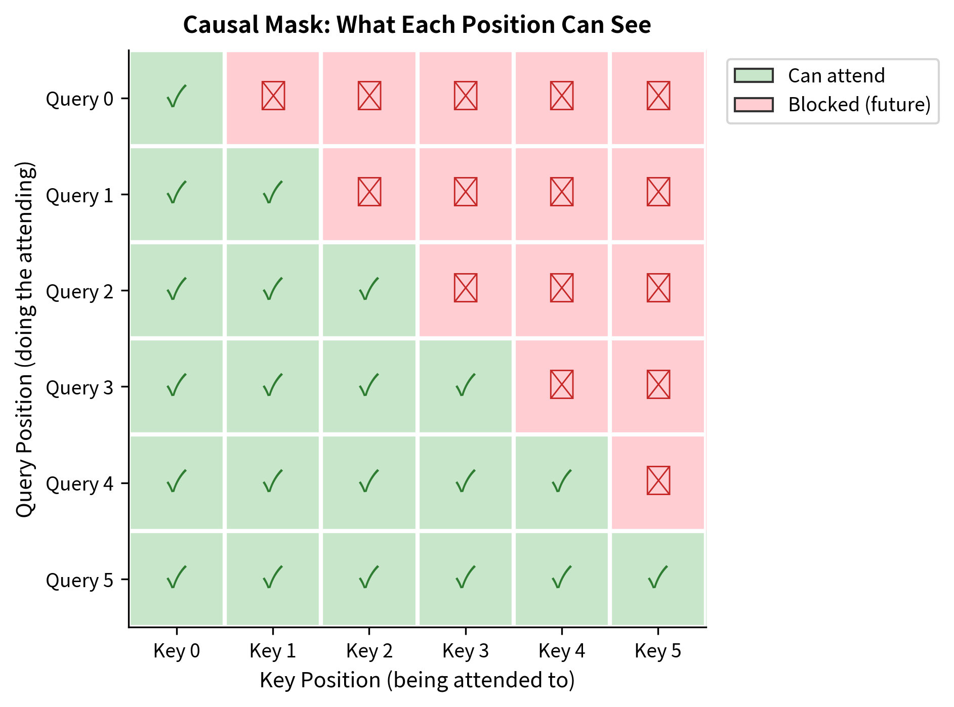
This creates a characteristic triangular pattern:
- Row 0 (first token): only column 0 is allowed (the token can only see itself)
- Row 1 (second token): columns 0 and 1 are allowed (can see itself and the first token)
- Row (last token): all columns 0 through are allowed (can see the entire sequence)
Why Creates Zero Attention
The mathematical trick is elegant. After adding the mask, we apply softmax to convert scores to attention weights. For a masked position:
As the mask value approaches , the numerator approaches 0. The denominator remains positive because unmasked positions contribute finite, positive exponentials. The result:
Those positions receive exactly zero attention weight. The token at position effectively cannot see any token at positions . In practice, we use a large finite value like instead of true infinity, which achieves the same effect with standard floating-point arithmetic.
Implementation
Let's implement causal masking and visualize the resulting attention pattern. The mask is simply an upper triangular matrix of negative infinities:
Position 0 can only attend to itself. Position 1 can attend to positions 0 and 1. Position 4 can attend to all five positions. The triangular structure ensures strictly left-to-right information flow.
Anatomy of a Decoder Block
Now that we understand causal masking, let's see how it fits into a complete decoder block. A decoder block is structurally similar to an encoder block, with one critical difference: its self-attention layer applies causal masking. But the block is more than just masked attention; it's a carefully designed composition of components that work together to transform token representations.
The Two-Sublayer Structure
Each decoder block consists of two sublayers that serve complementary purposes:
-
Causal Multi-Head Self-Attention: This sublayer enables cross-position communication. Each token gathers information from previous tokens (and itself), building a representation that incorporates relevant context. The causal mask ensures this communication respects temporal order.
-
Feed-Forward Network (FFN): This sublayer provides position-wise transformation. The same two-layer MLP is applied independently to each position, adding non-linear representational capacity. Unlike attention, the FFN doesn't mix information across positions; it processes each token's representation in isolation.
These sublayers address different aspects of representation learning. Attention handles where to look in the sequence. The FFN handles how to transform what was gathered. Together, they enable the block to both aggregate context and compute complex functions of that context.
Supporting Components
Two additional components wrap each sublayer to enable deep networks:
-
Residual Connections: Skip connections around each sublayer create additive shortcuts. Instead of computing , the block computes . This means the sublayer only needs to learn the delta, or refinement, to add to the representation. Residuals also provide direct gradient paths that bypass potentially problematic nonlinearities.
-
Layer Normalization: Normalizes activations to stabilize training. Modern decoders use Pre-LN architecture, applying normalization before each sublayer rather than after. Pre-LN produces more stable gradients at initialization and enables training without careful learning rate warmup.
The data flow through a Pre-LN decoder block follows this pattern:
- Normalize → Attention → Add residual
- Normalize → FFN → Add residual
Let's implement each component and assemble them into a complete decoder block.
Utility Functions
First, we need a few utility functions. The softmax function converts raw scores to probabilities. RMS normalization scales activations to have unit root-mean-square. GELU provides a smooth nonlinearity for the feed-forward network:
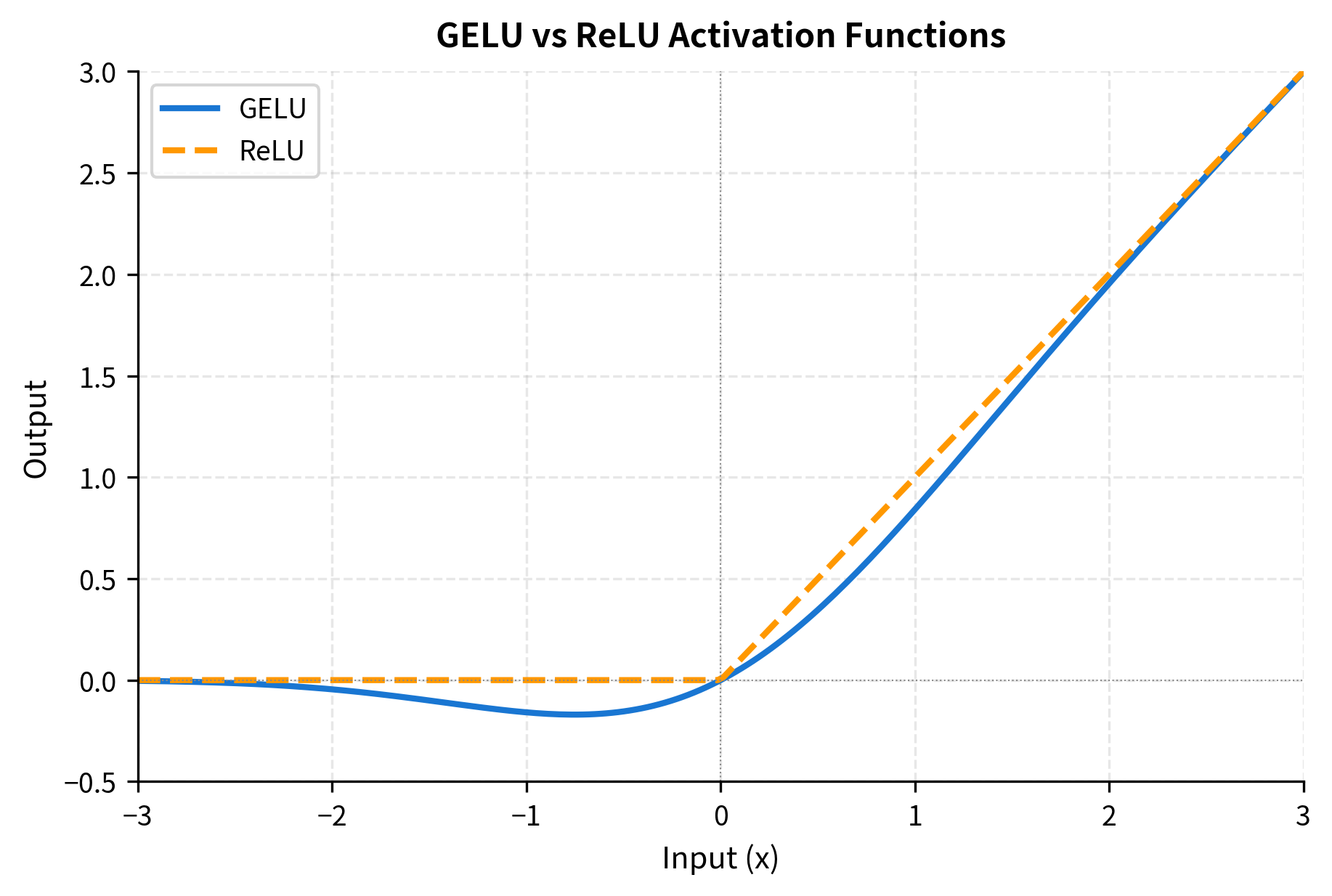
The smooth transition of GELU can improve gradient flow during training compared to ReLU's sharp corner at zero.
Causal Multi-Head Attention
The attention layer is the heart of the decoder block. It projects input tokens into queries, keys, and values, then computes attention with causal masking. Multiple heads allow the model to attend to different aspects of the context simultaneously:
The attention layer computes the same scaled dot-product attention as an encoder, but the causal mask ensures the upper triangle of attention weights becomes zero. Each position's output is a weighted sum of value vectors from itself and all previous positions.
Position-Wise Feed-Forward Network
After attention aggregates context, the FFN transforms each position independently. It expands the representation to a larger hidden dimension, applies a nonlinearity, then projects back to the model dimension. This expansion-contraction pattern adds significant representational capacity:
Assembling the Decoder Block
Now we combine attention, FFN, normalization, and residual connections into a complete decoder block. The Pre-LN architecture applies normalization before each sublayer, which produces more stable gradients and enables training without warmup:
Testing the Decoder Block
Let's instantiate a decoder block and verify it works correctly. We'll use typical hyperparameters: 256-dimensional model, 8 attention heads (32 dimensions each), and a 4x FFN expansion:
The block contains roughly 790K parameters, dominated by the feed-forward network (which uses a 4x expansion ratio: ). The input and output shapes match, allowing blocks to be stacked without dimension changes. This "residual-friendly" design is what enables deep networks: each block can refine the representation without fundamentally altering its structure.
The decoder block transforms each position independently while allowing controlled information flow from past positions through causal attention. The FFN adds non-linear transformation capacity without any cross-position interaction.
GPT-Style Decoder Architecture
GPT (Generative Pre-trained Transformer) established the dominant decoder-only paradigm. The full GPT architecture consists of:
- Token Embedding: Maps input token IDs to dense vectors
- Position Embedding: Adds positional information (learned or sinusoidal)
- Decoder Stack: Multiple decoder blocks in sequence
- Final Layer Norm: Normalizes the output of the last block
- Language Model Head: Projects to vocabulary size for next-token prediction
Let's build a complete GPT-style decoder.
The parameter count breaks down into three main components: embeddings (token + position), the decoder stack, and the language model head. With a 10K vocabulary and 256-dimensional embeddings, the token embedding alone accounts for 2.56M parameters. The 6 decoder blocks contribute about 4.7M parameters (roughly 790K each), and the LM head adds another 2.56M for projecting back to vocabulary size.
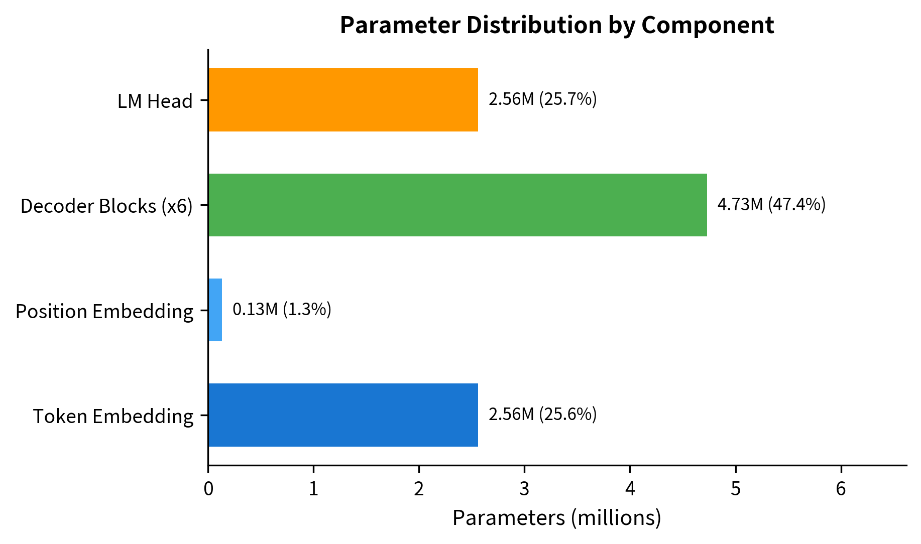
This 6.9M parameter model is tiny by modern standards. GPT-2 Small has 117M parameters, GPT-3 has 175B, and GPT-4 is estimated at over a trillion. But the architectural pattern is identical: stack more layers, increase dimensions, and scale up the training data.
Layer Stacking and Information Flow
Decoder blocks are stacked sequentially. The output of block becomes the input to block . Each layer refines the representations, building increasingly abstract features.
The representation norms reveal how the network transforms token embeddings. Starting from the embedding layer with relatively small norms (around 0.3), the representations grow as they pass through successive blocks. This growth reflects the accumulation of information via residual connections: each block adds its contribution to the running representation. The final layer norm rescales the output, ensuring consistent magnitudes before the language model head computes logits.
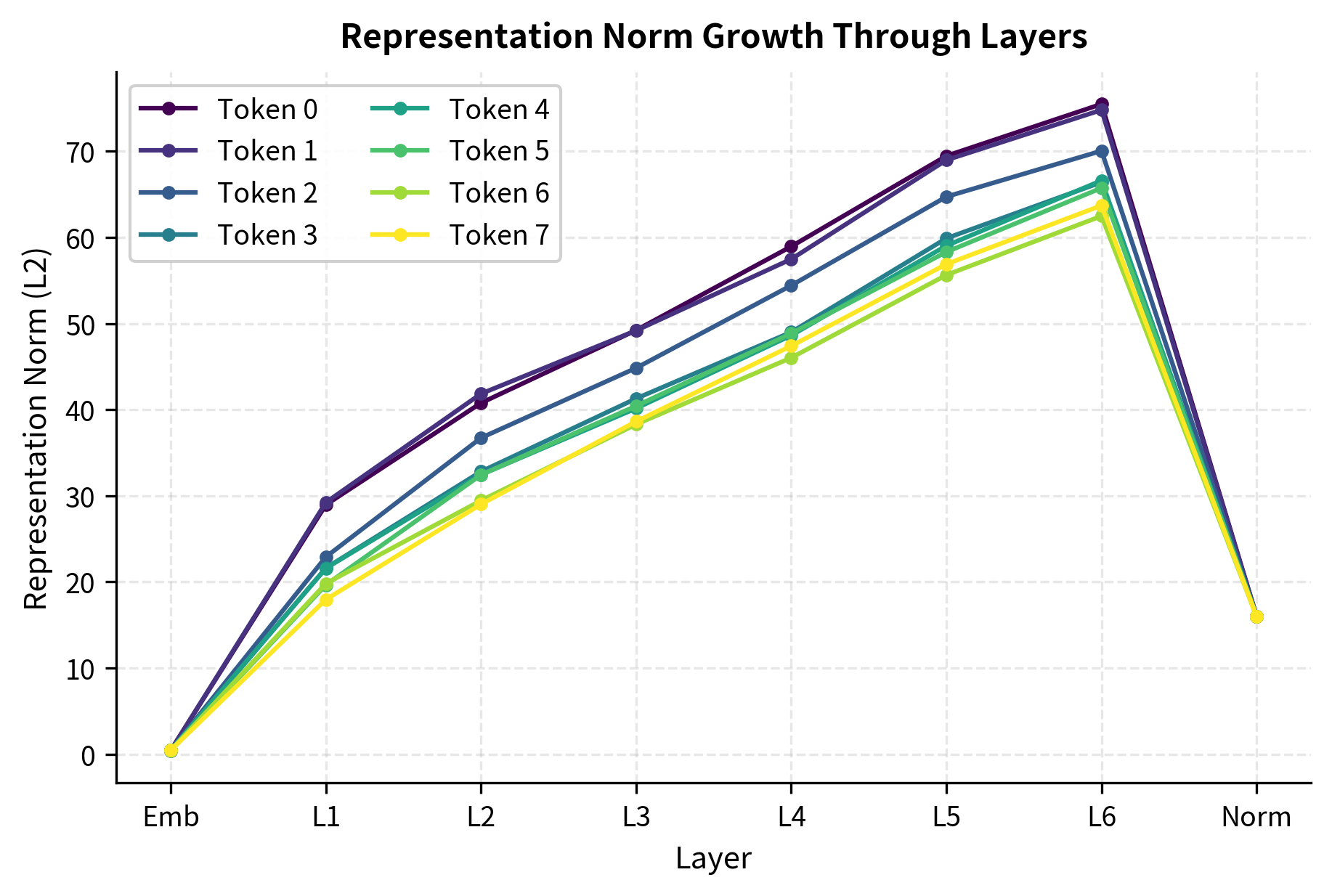
As we go deeper, representation norms tend to grow or stabilize depending on initialization and normalization. The final layer norm ensures consistent scale before the language model head.
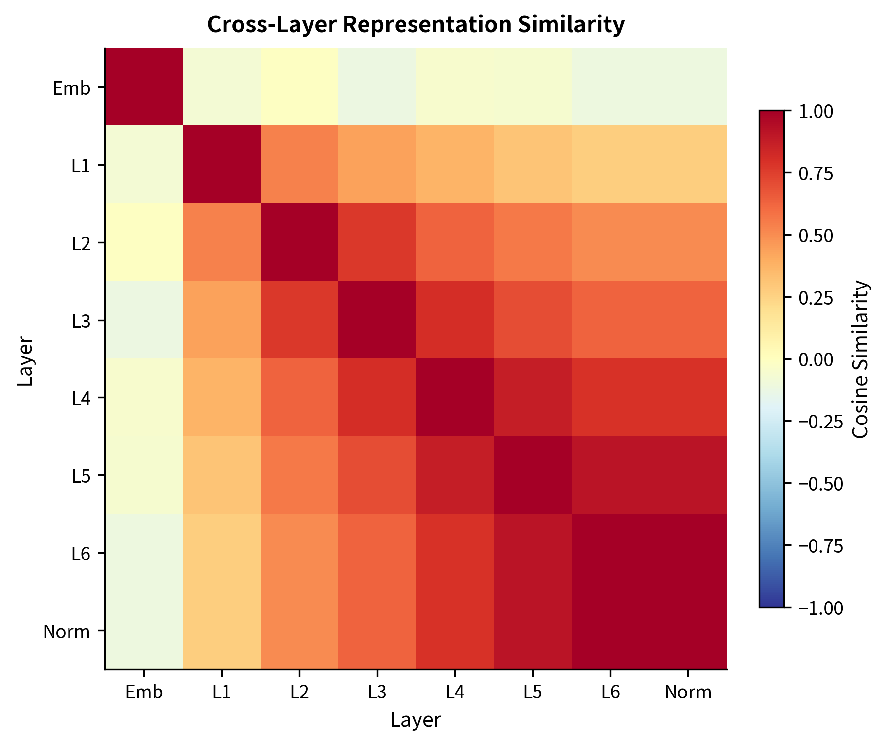
The similarity matrix reveals how representations evolve. Adjacent layers tend to be more similar (the residual connections preserve information), while distant layers may diverge significantly as the model builds higher-level abstractions.
Visualizing Causal Attention Patterns
Each attention head in a decoder develops specialized patterns. Some heads attend strongly to the previous token (local context). Others attend to the beginning of the sequence. Still others develop positional patterns or semantic groupings.
Let's examine attention patterns in a decoder block.
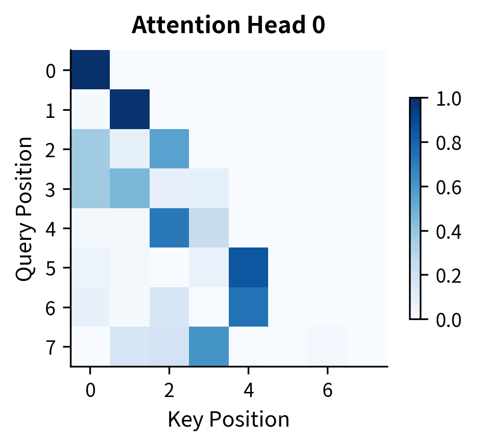
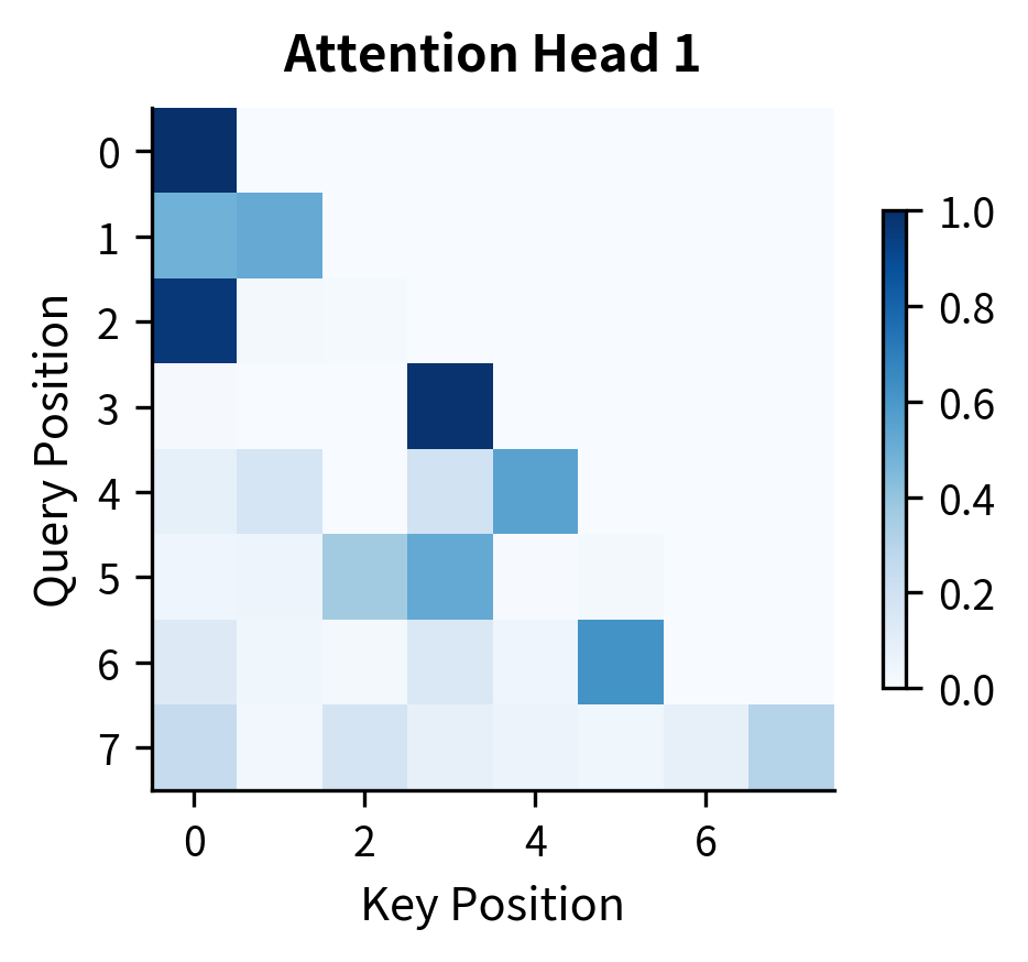
Both heads exhibit the causal structure with zeros in the upper triangle. The intensity patterns within the lower triangle vary between heads, showing how different heads attend to different parts of the available context. With random initialization, these patterns are not yet meaningful, but training shapes them into useful attention strategies.
The Generation Loop
At inference time, the decoder generates text autoregressively. Each iteration:
- Processes the current sequence through all decoder blocks
- Takes the logits at the final position
- Samples or greedily selects the next token
- Appends that token to the sequence
- Repeats until a stopping condition
The model generated 10 new tokens from the 3-token prompt. Since this is a randomly initialized model (not trained on any text), the generated token IDs are essentially random samples from the vocabulary. A trained model would produce coherent continuations. The temperature of 0.8 makes the distribution slightly sharper than pure random sampling, biasing toward higher-probability tokens.
Let's visualize how temperature affects the sampling distribution. Lower temperatures concentrate probability mass on the highest-scoring tokens, while higher temperatures flatten the distribution:
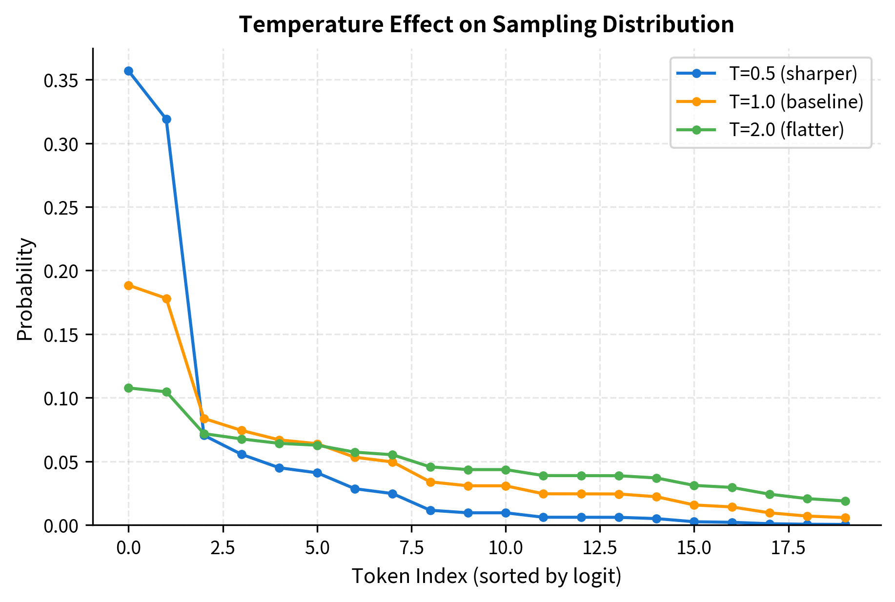
At temperature 0.5, the top tokens dominate the distribution, making generation more deterministic. At temperature 2.0, even low-scoring tokens have non-negligible probability, introducing more randomness and diversity. The choice of temperature trades off between coherence (low temperature) and creativity (high temperature).
In practice, generation involves beam search, top-k sampling, nucleus sampling, and other decoding strategies to balance quality and diversity. The decoder architecture itself doesn't change; only the sampling logic varies.
Key-Value Caching for Efficient Generation
A naive implementation recomputes attention for all positions at every generation step. This is wasteful: the representations for tokens 0 through don't change when we add token . KV caching stores the key and value vectors from previous positions, avoiding redundant computation.
The cache grows from shape (4, 5, 16) to (4, 6, 16) after adding one token. Here, 4 is the number of heads, the middle dimension is sequence length (growing from 5 to 6), and 16 is the head dimension (64 / 4 heads). When processing the new token, we only compute queries for that single position, but the keys and values span all 6 positions. This asymmetry is what makes caching efficient: the expensive key-value computation for old tokens is reused.
With KV caching, generating new tokens requires compute instead of , where:
- : the number of new tokens to generate
- : the total sequence length (prompt plus generated tokens)
- : linear scaling because each new token only computes attention against the cached keys/values
- : quadratic scaling without caching, since we recompute all positions at each step
This optimization is critical for efficient inference in production systems. For a 1000-token prompt with 100 generated tokens, caching reduces attention computation by roughly 50x.
Decoder Architecture Comparison
Different models use slightly different decoder designs. The core pattern is consistent, but details vary:
| Model | Layers | Heads | FFN Ratio | Norm | Notable Features | |
|---|---|---|---|---|---|---|
| GPT-2 Small | 12 | 12 | 768 | 4x | Layer Norm | Learned position embeddings |
| GPT-2 Medium | 24 | 16 | 1024 | 4x | Layer Norm | Pre-LN architecture |
| GPT-3 | 96 | 96 | 12288 | 4x | Layer Norm | Sparse attention in some heads |
| Llama 2 7B | 32 | 32 | 4096 | 2.7x | RMSNorm | RoPE, SwiGLU FFN |
| Llama 3 8B | 32 | 32 | 4096 | 3.5x | RMSNorm | Grouped-query attention |
| Mistral 7B | 32 | 32 | 4096 | 3.5x | RMSNorm | Sliding window attention |
Modern decoders favor RMSNorm over LayerNorm for efficiency, SwiGLU or GeGLU activations in the FFN for better performance, and positional encodings like RoPE that generalize to longer sequences. Grouped-query attention reduces the KV cache size by sharing key-value projections across groups of heads.
When to Use Decoder-Only Models
Decoder-only architectures excel at:
- Text generation: Stories, code, conversations, completions
- Language modeling: Predicting the next token given context
- In-context learning: Few-shot learning through prompting
- General-purpose AI assistants: Handling diverse tasks through natural language
They are less naturally suited for:
- Bidirectional understanding: Tasks like named entity recognition or question answering over a document, where seeing the full context helps
- Sequence-to-sequence with misaligned lengths: Machine translation where the source and target have different structures
- Fixed-length encoding: Producing a single vector representation of a document
For these tasks, encoder-only (like BERT) or encoder-decoder models (like T5) may be more appropriate. However, large decoder-only models trained with instruction tuning have proven surprisingly capable across task types, blurring these traditional boundaries.
Limitations and Impact
The decoder-only architecture has transformed language AI, but it comes with inherent constraints that shape both its capabilities and its failure modes.
The autoregressive nature means generation is inherently sequential at inference time. Each new token depends on all previous tokens, preventing parallel generation. While KV caching mitigates redundant computation, the fundamental serial dependency remains. For real-time applications, this creates latency constraints that scale with output length. Techniques like speculative decoding, where a smaller model drafts tokens that a larger model verifies in parallel, partially address this, but the sequential bottleneck persists.
Causal masking also limits the model's understanding of each position. When processing position , the decoder cannot consider positions even though, for understanding tasks, that future context would be valuable. Bidirectional models like BERT can leverage the full context for each position, giving them an advantage for tasks like classification or extraction. Decoder-only models compensate through scale and training data, but the architectural constraint remains.
Despite these limitations, the decoder-only paradigm has proven remarkably versatile. The GPT series demonstrated that next-token prediction at scale produces emergent capabilities in reasoning, code generation, and multilingual understanding. The simplicity of the architecture, a single stack of nearly identical blocks, enables efficient scaling and has become the foundation for modern generative AI. From GPT-2's surprising text generation to GPT-4's multimodal reasoning, the decoder architecture continues to define the frontier of language AI.
Key Parameters
When configuring a decoder-only transformer, the following parameters have the greatest impact on model capacity and performance:
-
d_model (model dimension): The dimensionality of token representations throughout the network. Common values range from 256 (small models) to 12288 (GPT-3 scale). Must be divisible by
n_heads. Larger values increase capacity but quadratically increase attention computation. -
n_heads (number of attention heads): How many parallel attention patterns the model can learn. Typically set so that
d_model / n_headsyields head dimensions of 64-128. More heads enable diverse attention patterns but have diminishing returns beyond a point. -
n_layers (number of decoder blocks): The depth of the transformer stack. Deeper models learn more abstract representations. GPT-2 Small uses 12 layers; GPT-3 uses 96. Depth trades off against width for a given parameter budget.
-
d_ff (feed-forward hidden dimension): The expansion dimension in the FFN sublayer. Traditionally 4x
d_model, but modern models use 2.7x-3.5x with gated activations like SwiGLU. Larger FFN dimensions increase the network's non-linear transformation capacity. -
vocab_size: The number of tokens in the vocabulary. Larger vocabularies reduce sequence length for the same text but increase embedding and LM head parameters. Typical values range from 30K (GPT-2) to 128K (Llama 3).
-
max_seq_len: Maximum sequence length the model can process. Affects position embedding size and memory requirements during training. Modern models support 2K-128K tokens through efficient attention mechanisms.
-
temperature (generation): Controls randomness during sampling. Values below 1.0 sharpen the distribution (more deterministic); values above 1.0 flatten it (more random). Common range is 0.7-1.0 for generation tasks.
Summary
The decoder architecture powers modern language generation by combining self-attention with causal masking to enforce left-to-right information flow. Key takeaways:
- Causal masking prevents each position from attending to future positions, matching the autoregressive generation process
- Decoder blocks consist of masked self-attention and feed-forward layers, each with residual connections and normalization
- GPT-style models stack decoder blocks between embedding and language model head layers, forming a unified architecture for understanding and generation
- Layer stacking builds increasingly abstract representations, with each layer refining outputs from the previous layer
- KV caching enables efficient generation by storing key-value pairs from previous positions
- Generation proceeds token by token, with each new token conditioned on all previous ones through the attention mechanism
The decoder-only design has become the default architecture for large language models, offering simplicity, scalability, and surprising generality. While encoder and encoder-decoder architectures retain advantages for specific tasks, the decoder's unified approach to understanding and generation has proven remarkably effective across the spectrum of language AI applications.
Quiz
Ready to test your understanding? Take this quick quiz to reinforce what you've learned about decoder architectures and causal masking.

Comments