Scaled Dot-Product Attention: The Core Transformer Mechanism

In the previous chapter, we explored the fundamental pattern of self-attention: compute similarity scores, normalize with softmax, and aggregate values. We used raw embeddings directly, measuring similarity through dot products between embedding vectors. This simplified approach captures the essence of attention, but real transformer models use a more powerful formulation called scaled dot-product attention.

This refinement introduces two key modifications. First, instead of using embeddings directly, we project them into three separate representations: queries, keys, and values. Second, we scale the dot products before applying softmax to prevent numerical instability. These changes might seem minor, but they're essential for training deep attention-based models effectively.

The insight behind queries, keys, and values comes from information retrieval. Think of a database lookup: you have a query (what you're searching for), a set of keys (labels for stored items), and values (the actual stored content). The lookup process finds keys that match the query and returns the corresponding values.

Self-attention works similarly. For each position in the sequence:

• The query represents what this position is "looking for"
• The keys represent what each position "offers" to be matched against
• The values represent the information each position will contribute to the output

Why not just use the embeddings directly, as we did in the simplified version? The separate projections give the model more flexibility. The query projection can learn to emphasize features that are useful for finding relevant context. The key projection can learn to emphasize features that are useful for being found. And the value projection can learn what information is actually useful to contribute to the output. These are different roles, and separating them allows the model to specialize each representation.

Given an input sequence of $n$ tokens with $d$-dimensional embeddings, we create queries, keys, and values through learned linear transformations:

where:

• $X \in \mathbb{R}^{n \times d}$ is the input embedding matrix (rows are token embeddings)
• $W^Q \in \mathbb{R}^{d \times d_k}$ projects inputs to queries
• $W^K \in \mathbb{R}^{d \times d_k}$ projects inputs to keys
• $W^V \in \mathbb{R}^{d \times d_v}$ projects inputs to values
• $Q \in \mathbb{R}^{n \times d_k}$ is the query matrix
• $K \in \mathbb{R}^{n \times d_k}$ is the key matrix
• $V \in \mathbb{R}^{n \times d_v}$ is the value matrix

The dimensions $d_k$ (key/query dimension) and $d_v$ (value dimension) are hyperparameters. Often $d_k = d_v = d$, but they can differ. The critical requirement is that queries and keys must have the same dimension $d_k$ since we'll compute their dot products.

Each token's embedding gets transformed into three distinct vectors. Position $i$ produces query $\mathbf{q}_i$, key $\mathbf{k}_i$, and value $\mathbf{v}_i$. The query will be used to find relevant positions; the key will be used to be found; the value will be used to contribute information.

With queries and keys in hand, we need a way to measure how relevant each key is to each query. The dot product provides exactly this: it quantifies how much two vectors point in the same direction. For query $\mathbf{q}_i$ and key $\mathbf{k}_j$, the similarity score is:

where:

• $s_{ij}$: the similarity score between position $i$'s query and position $j$'s key
• $\mathbf{q}_i$: the query vector for position $i$, a $d_k$-dimensional vector
• $\mathbf{k}_j$: the key vector for position $j$, also $d_k$-dimensional
• $q_{il}$: the $l$-th component of query $\mathbf{q}_i$
• $k_{jl}$: the $l$-th component of key $\mathbf{k}_j$
• $d_k$: the dimension of query and key vectors

The dot product measures alignment: if the query and key point in similar directions, the score is high and positive. If they're orthogonal (perpendicular in the $d_k$-dimensional space), the score is zero. If they point in opposite directions, the score is negative.

To compute all $n^2$ pairwise similarity scores at once, we use matrix multiplication:

where:

• $S \in \mathbb{R}^{n \times n}$: the score matrix containing all pairwise similarities
• $Q \in \mathbb{R}^{n \times d_k}$: the query matrix (rows are query vectors)
• $K^T \in \mathbb{R}^{d_k \times n}$: the transposed key matrix (columns are key vectors)

Entry $s_{ij}$ in the resulting matrix tells us how much position $i$'s query matches position $j$'s key. This single matrix multiplication replaces $n^2$ individual dot products.

The score matrix shows the raw dot products between all query-key pairs. Some values are positive (similar directions), others negative (opposite directions). Before we can use these as attention weights, we need to apply softmax. But there's a problem we need to address first.

Consider what happens as the dimension $d_k$ grows. Each dot product is a sum of $d_k$ terms:

where:

• $\mathbf{q}$: a query vector of dimension $d_k$
• $\mathbf{k}$: a key vector of dimension $d_k$
• $q_l$: the $l$-th component of the query vector
• $k_l$: the $l$-th component of the key vector
• $d_k$: the number of dimensions in the query/key space

If the individual components $q_l$ and $k_l$ have unit variance (which is typical after proper initialization), then each product $q_l k_l$ has variance around 1. The sum of $d_k$ independent terms with variance 1 has variance $d_k$. This means the dot product's magnitude scales with $\sqrt{d_k}$.

Let's verify this empirically:

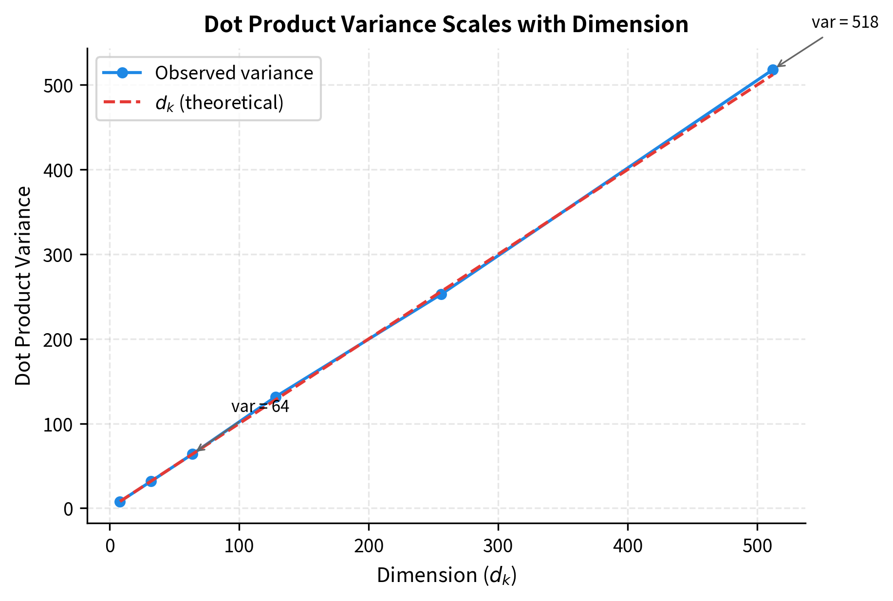
The variance grows exactly as predicted: for $d_k = 512$, the variance is approximately 512. This means dot products can easily reach magnitudes of 30 or more (since $\sqrt{512} \approx 23$).

Why does this matter? The softmax function converts scores to probabilities:

where:

• $\alpha_{ij}$: the attention weight from position $i$ to position $j$ (how much position $i$ attends to position $j$)
• $s_{ij}$: the raw similarity score between position $i$'s query and position $j$'s key
• $\exp(s_{ij})$: the exponential of the score, ensuring positivity
• $\sum_{k=1}^{n} \exp(s_{ik})$: the sum over all $n$ positions, normalizing so weights sum to 1

Large input values push softmax into its saturated regime. If one score is significantly larger than the others, the exponential blows up that difference. Consider scores [10, 1, 1, 1]: after softmax, the weights become approximately [0.9999, 0.0001, 0.0001, 0.0001]. The attention becomes nearly one-hot, attending almost exclusively to a single position.

This extreme behavior causes two problems during training. First, gradients become vanishingly small in the saturated regions of softmax, slowing learning. Second, the model loses the ability to express soft, distributed attention patterns. It can only focus sharply on one thing.

With small scores, attention distributes across positions with the highest weight around 0.41 and entropy around 1.26 (fairly distributed). With large scores, attention collapses: the maximum weight approaches 1.0 and entropy drops to nearly 0 (extremely peaked). The model can no longer express nuanced attention patterns.

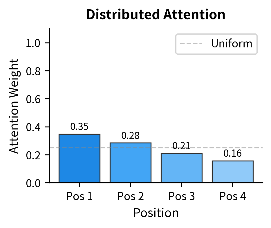
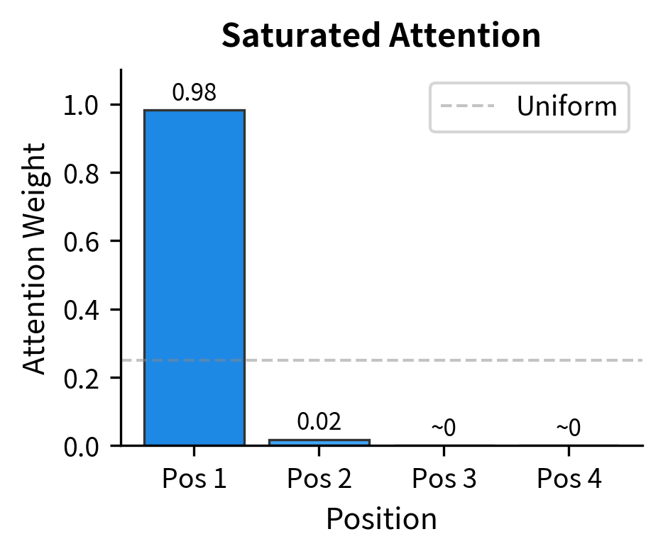
The visualization makes the contrast stark. With small scores, attention is roughly distributed across all four positions. With large scores (20x larger), almost all attention flows to position 1, with the other positions receiving essentially zero weight. This is why scaling is essential: without it, high-dimensional embeddings produce scores so large that softmax always saturates.

The solution is straightforward: divide the dot products by $\sqrt{d_k}$ before applying softmax. Since the dot product variance is $d_k$, dividing by $\sqrt{d_k}$ brings the variance back to 1:

where:

• $\text{Var}(\cdot)$: the variance operator
• $\mathbf{q} \cdot \mathbf{k}$: the dot product between a query and key vector
• $d_k$: the dimension of query and key vectors
• $\sqrt{d_k}$: the scaling factor applied to the dot product

The key property used here is that when you divide a random variable by a constant $c$, its variance is divided by $c^2$. Since we divide by $\sqrt{d_k}$, the variance is divided by $(\sqrt{d_k})^2 = d_k$.

With unit-variance scores, softmax operates in its sensitive region where small changes in scores produce meaningful changes in weights. The model can learn both sharp and soft attention patterns.

Let's derive why the dot product has variance $d_k$. Assume $q_l$ and $k_l$ are independent random variables with zero mean and unit variance (typical after proper weight initialization).

Step 1: Variance of a single product term

For a single component product $q_l k_l$:

• Mean: $\mathbb{E}[q_l k_l] = \mathbb{E}[q_l] \cdot \mathbb{E}[k_l] = 0 \times 0 = 0$ (by independence)
• Variance: $\text{Var}(q_l k_l) = \mathbb{E}[q_l^2 k_l^2] - \mathbb{E}[q_l k_l]^2 = \mathbb{E}[q_l^2] \cdot \mathbb{E}[k_l^2] - 0 = 1 \times 1 = 1$

Each product term has zero mean and unit variance.

Step 2: Variance of the sum (the dot product)

The dot product $\mathbf{q} \cdot \mathbf{k} = \sum_{l=1}^{d_k} q_l k_l$ sums $d_k$ independent terms. When summing independent random variables, variances add:

Step 3: Effect of scaling

Dividing by $\sqrt{d_k}$ scales the variance by $1/d_k$:

This is why the "Attention Is All You Need" paper prescribes exactly this scaling factor: it ensures unit-variance scores regardless of the embedding dimension.

We've now assembled all the pieces: queries that search for relevant context, keys that advertise what each position offers, values that carry the actual information, dot products that measure relevance, scaling that keeps softmax well-behaved, and softmax that converts scores to weights. The complete mechanism chains these operations together into a single formula.

Consider what we need to accomplish for each position in the sequence:

1. Find relevant positions: Compare this position's query against all keys
2. Determine importance: Convert raw similarities into attention weights
3. Gather information: Blend all values according to those weights

The formula that captures this entire process is:

where:

• $Q \in \mathbb{R}^{n \times d_k}$: the query matrix, with one row per position
• $K \in \mathbb{R}^{n \times d_k}$: the key matrix, with one row per position
• $V \in \mathbb{R}^{n \times d_v}$: the value matrix, containing information to aggregate
• $d_k$: the dimension of queries and keys (must match for dot product)
• $d_v$: the dimension of values (can differ from $d_k$)
• $n$: the sequence length (number of tokens)
• $\text{softmax}$: applied row-wise to convert scores to probability distributions

This formula is read from the inside out, following the order of operations. Let's trace through each stage to understand how the pieces fit together.

Stage 1: Compute pairwise similarities with $QK^T$

The matrix multiplication $QK^T$ computes all $n^2$ query-key dot products simultaneously. When we multiply a query matrix of shape $(n, d_k)$ by a transposed key matrix of shape $(d_k, n)$, we get a score matrix of shape $(n, n)$. Entry $(i, j)$ contains the dot product $\mathbf{q}_i \cdot \mathbf{k}_j$, measuring how much position $i$ should attend to position $j$.

Stage 2: Normalize variance with $/\sqrt{d_k}$

Before applying softmax, we divide all scores by $\sqrt{d_k}$. As we derived earlier, this keeps the score variance at 1 regardless of dimension, preventing softmax from saturating. Without this scaling, high-dimensional queries and keys would produce scores so large that softmax collapses to near-one-hot distributions.

Stage 3: Convert to probabilities with $\text{softmax}(\cdot)$

Softmax is applied row-wise, so each row of the score matrix becomes an independent probability distribution. Row $i$ tells us how position $i$ distributes its attention across all positions. The weights are positive and sum to 1, making them valid for computing weighted averages.

Stage 4: Aggregate values with $\cdot V$

Finally, we multiply the $n \times n$ attention weight matrix by the $n \times d_v$ value matrix. This computes, for each position, a weighted sum of all value vectors. The result is an $n \times d_v$ matrix where row $i$ is position $i$'s new representation, enriched with information gathered from across the sequence.

The output is a matrix where each row is the contextual representation for one position, computed as a weighted average of all value vectors according to the attention weights.

Translating this formula into code reveals its simplicity. Three matrix operations capture the entire attention mechanism:

The implementation is concise. One matrix multiplication computes all pairwise scores, scalar division handles scaling, softmax normalizes each row, and a final matrix multiplication aggregates the values. This composability is what makes attention so powerful: complex contextual reasoning emerges from simple, differentiable operations.

Let's apply this function to our running example and examine the outputs:

The attention weight matrix has shape $(4, 4)$: one row for each of our 4 tokens, one column for each potential attention target. Each row sums to exactly 1.0, confirming that softmax produces valid probability distributions. The output has shape $(4, 6)$, matching our sequence length and value dimension. Each position now carries a contextual representation that blends information from all positions, with the blending proportions determined by the attention weights.

Let's trace through the complete attention computation visually. We'll use a small example with interpretable tokens to see how each step transforms the data.

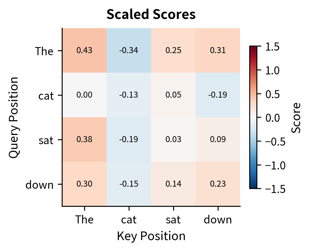
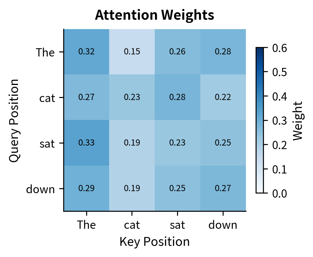
The left panel shows scaled similarity scores ranging roughly from -1 to +1. This moderate range keeps softmax well-behaved. The right panel shows attention weights after softmax, where each row forms a probability distribution. Some positions focus attention sharply (one dominant weight), while others distribute attention more broadly.

The formula $\text{Attention}(Q, K, V) = \text{softmax}(QK^T/\sqrt{d_k})V$ computes everything through matrix multiplications, which are highly optimized on modern hardware.

Let's trace the shapes through the computation:

The attention weight matrix is $n \times n$, which is the source of the quadratic complexity we discussed in the previous chapter. For sequence length $n = 100$, this is a $100 \times 100 = 10,000$ element matrix. For $n = 10,000$ (a moderately long document), it becomes 100 million elements.

However, note that the computations are batch-able. In practice, we process multiple sequences simultaneously:

Batched operations leverage GPU parallelism effectively. All three sequences are processed simultaneously through the same matrix multiplications.

The formula becomes concrete when we trace through it with actual numbers. Let's work through a minimal example: three tokens with 2-dimensional queries, keys, and values. By keeping the dimensions tiny, we can follow every calculation by hand and build intuition for what the attention mechanism actually computes.

We'll work with three abstract tokens, "A," "B," and "C." In a real model, these would come from learned projections of input embeddings. Here, we'll define them directly with carefully chosen values that have geometric meaning.

The queries have an intuitive geometric interpretation: "A" points due east (along dimension 1), "C" points due north (along dimension 2), and "B" points northeast (equally between both dimensions). The keys are distributed similarly but with different magnitudes. The values are orthogonal basis vectors plus a midpoint, making it easy to see how blending works.

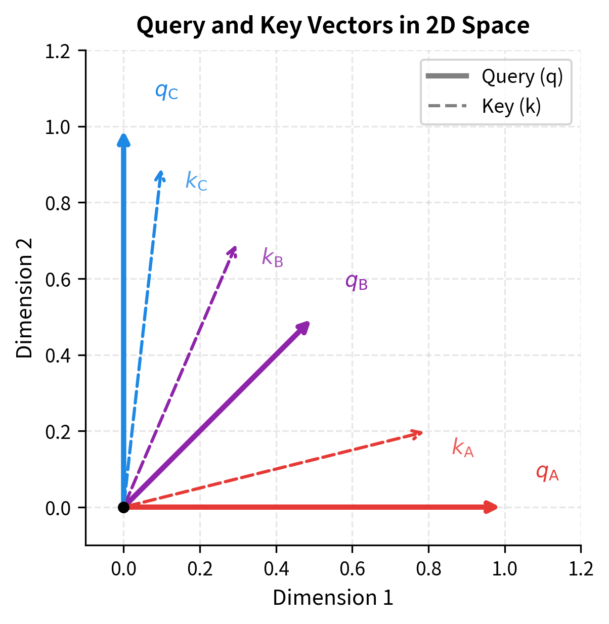
The visualization reveals why certain query-key pairs have high dot products. Query $q_A$ points east and aligns well with key $k_A$ (which also has a strong eastward component), producing a high similarity score. Query $q_C$ points north and aligns best with key $k_C$ (which points mostly north). Query $q_B$ lies between the axes and has moderate similarity with all keys.

First, we compute the dot product between every query and every key. This measures how well each query-key pair aligns.

Token "A" (with its eastward query) has the highest similarity with key "A" (which also points mostly east) and lowest similarity with key "C" (which points mostly north). This makes geometric sense: parallel vectors have high dot products, perpendicular vectors have low dot products.

Next, we divide all scores by $\sqrt{d_k} = \sqrt{2} \approx 1.41$. With only 2 dimensions, this scaling is modest, but it becomes crucial in high-dimensional settings.

The scaled scores are smaller in magnitude, keeping them in a range where softmax will produce meaningful gradients. In our 2D example, scores that were around 0.8 become around 0.57. The relative ordering is preserved, but the absolute differences are compressed.

Softmax transforms each row of scaled scores into a probability distribution. Let's trace through the calculation for token "A" in detail.

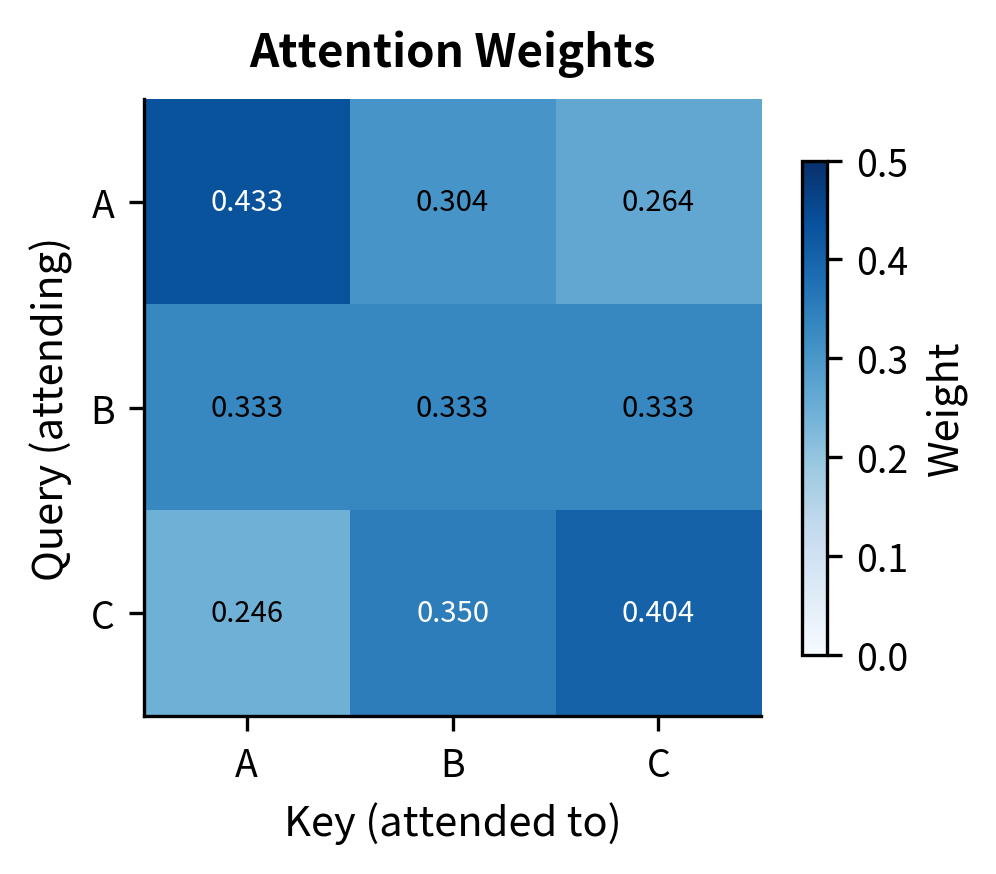
Each row now sums to 1.0, forming a valid probability distribution. Token "A" attends most strongly to itself (because its query aligned best with its own key), but it also gathers some information from "B" and "C." The attention isn't one-hot; it's a soft distribution that blends information from multiple sources.

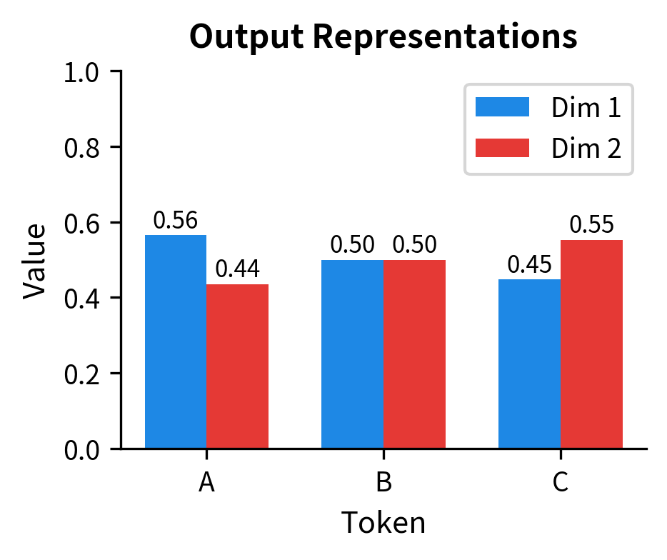
Finally, we use the attention weights to compute a weighted average of all value vectors for each position.

Token "A" started with value $[1.0, 0.0]$ but now has an output that incorporates information from all three positions. The output is approximately $[0.52, 0.48]$, reflecting the weighted blend of "A"'s value (weighted ~0.37), "B"'s value (weighted ~0.32), and "C"'s value (weighted ~0.31). The original position-specific information has been enriched with contextual information from the entire sequence.

To solidify why scaling matters, let's compare attention patterns with and without the $1/\sqrt{d_k}$ factor at different dimensions.

Without scaling, score standard deviation grows with $\sqrt{d_k}$, reaching over 22 at $d_k = 512$. This pushes the maximum attention weight toward 1.0, meaning attention collapses to near-one-hot. With scaling, score standard deviation stays around 1.0, and maximum weights remain moderate, allowing distributed attention patterns.

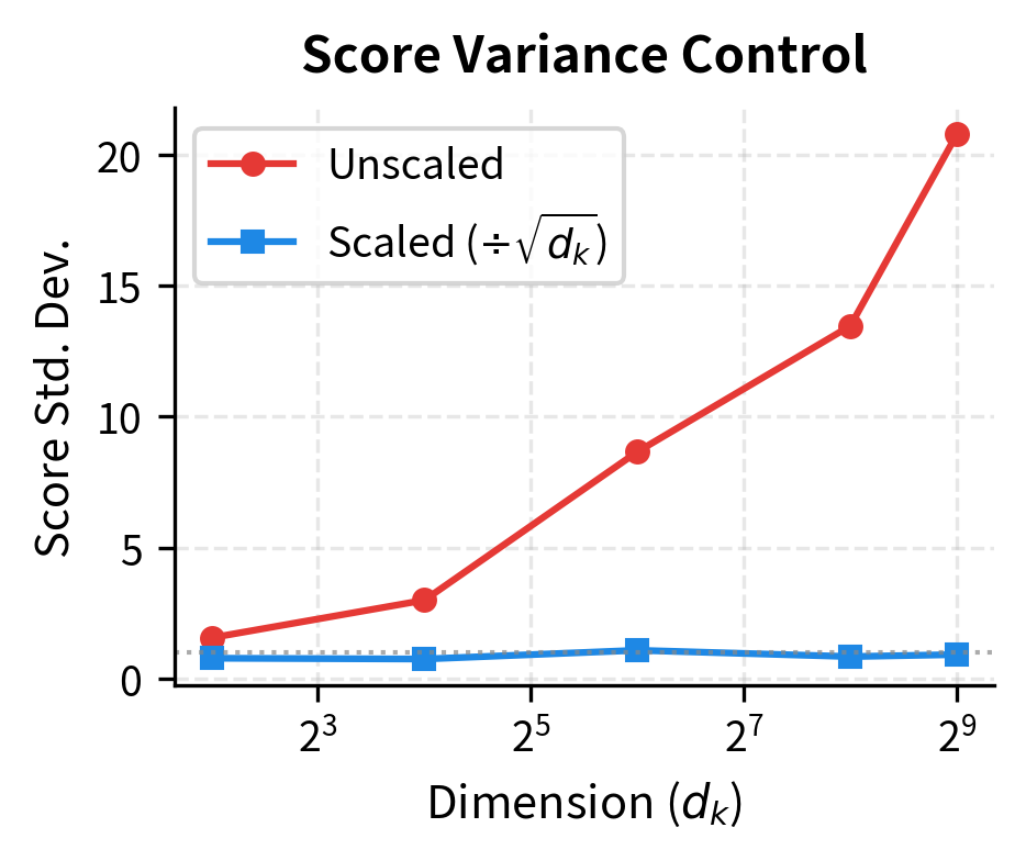
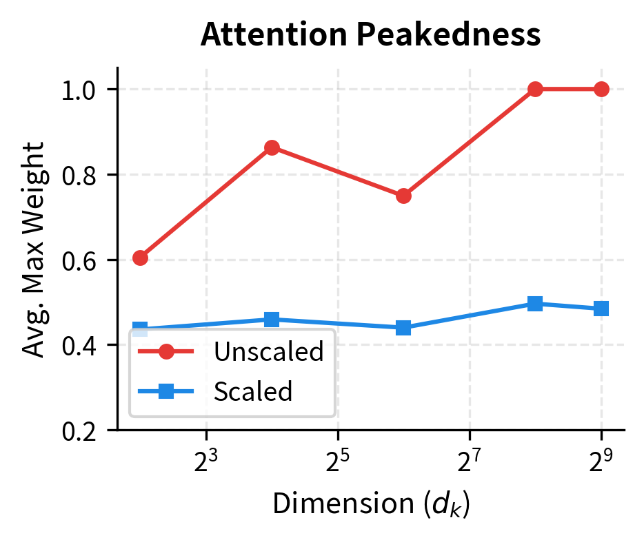
The visualization shows the benefit of scaling clearly. Without it, high-dimensional attention degenerates into hard selection. With it, the model retains the flexibility to express soft, distributed attention patterns throughout training.

Having traced through the formula by hand, we can now build a complete, reusable implementation. This module combines everything we've learned: it takes raw embeddings as input, projects them to queries, keys, and values, computes scaled dot-product attention, and returns contextualized representations.

A self-contained attention module needs three components:

1. Projection matrices: Learned parameters that transform input embeddings into Q, K, and V
2. The attention computation: The formula we've been studying
3. Proper initialization: Weight scaling that maintains signal magnitude through the network

The implementation follows patterns used in production transformer libraries like PyTorch and TensorFlow:

The __init__ method creates the three projection matrices with Xavier/Glorot initialization, which scales weights by $\sqrt{2/(d_{in} + d_{out})}$ to maintain variance through the network. The __call__ method implements the complete attention pipeline in just five lines: three projections, one scored dot product with scaling, and one value aggregation.

Let's verify that our implementation works correctly on a realistic example:

The module transforms our 8-token sequence with 32-dimensional embeddings into 8 contextualized representations with 16 dimensions each. The attention weights form an $8 \times 8$ matrix where each row sums to exactly 1.0, confirming that softmax produces valid probability distributions.

This implementation captures the mathematical essence of attention, but production systems add several refinements:

• Dropout: Applied to attention weights during training for regularization
• Batch processing: Handling multiple sequences simultaneously for GPU efficiency
• Autograd integration: Enabling gradient computation for backpropagation
• Numerical precision: Using half-precision floats for memory efficiency on large models

A later chapter on multi-head attention builds directly on this single-head foundation, showing how running multiple attention heads in parallel gives the model different "perspectives" on the same input sequence.

Scaled dot-product attention is the workhorse of modern NLP. The formula $\text{softmax}(QK^T/\sqrt{d_k})V$ encodes both what to attend to (through query-key matching) and what information to gather (through value aggregation). The scaling factor ensures stable training across different embedding dimensions, and the matrix formulation enables efficient GPU parallelization.

The mechanism has several important limitations to keep in mind. The $O(n^2)$ complexity in sequence length remains a fundamental constraint, where $n$ is the number of tokens. While the scaling factor helps with numerical stability, it doesn't reduce the quadratic memory and compute requirements. A 4,000-token sequence requires 16 million attention score computations, and an 8,000-token sequence requires 64 million. This motivates research into efficient attention variants like sparse attention, linear attention, and sliding window approaches.

Additionally, standard dot-product attention treats all positions symmetrically. Without positional encodings (covered in a later chapter), the model cannot distinguish "dog bites man" from "man bites dog." The attention mechanism itself is permutation-equivariant: shuffling input positions merely shuffles the output in the same way. External positional information must be injected to break this symmetry.

Despite these constraints, scaled dot-product attention unlocked the transformer architecture and the modern era of large language models. By enabling parallel processing of sequences and providing direct connections between any two positions, it solved the long-range dependency problems that limited recurrent models. The mechanism is simple enough to implement in a few lines of code, yet powerful enough to serve as the foundation for GPT, BERT, and their successors.

Scaled dot-product attention extends the basic attention mechanism with two key refinements: query-key-value projections and score scaling.

Key takeaways from this chapter:

• Query-Key-Value framework: Instead of using embeddings directly, we project them into specialized representations. Queries encode "what I'm looking for," keys encode "what I offer," and values encode "what information I contribute."

• Dot product for similarity: The similarity between query $i$ and key $j$ is their dot product $\mathbf{q}_i \cdot \mathbf{k}_j$. In matrix form, $QK^T$ computes all $n^2$ pairwise similarities efficiently.

• Scaling factor $1/\sqrt{d_k}$: Dot product variance grows with dimension $d_k$, causing softmax saturation in high dimensions. Dividing by $\sqrt{d_k}$ normalizes scores to unit variance, keeping softmax in its sensitive region.

• The attention formula: $\text{Attention}(Q, K, V) = \text{softmax}(QK^T/\sqrt{d_k})V$ combines scoring, normalization, and aggregation into a single differentiable operation.

• Matrix efficiency: The formula translates directly to matrix multiplications, enabling efficient batch processing on GPUs.

• Quadratic complexity: Computing $QK^T$ requires $O(n^2)$ operations for sequence length $n$. This remains the primary computational bottleneck for long sequences.

In the next chapter, we'll explore attention masking, which allows us to control which positions can attend to which. This is essential for causal language models (where future tokens must not influence past predictions) and for handling variable-length sequences in batches.

When implementing scaled dot-product attention, several hyperparameters control the model's capacity and behavior:

• $d_k$ (query/key dimension): Controls the dimensionality of the query and key projections. Larger values increase model capacity but also increase computation. Common choices range from 64 to 128 per attention head. The scaling factor $1/\sqrt{d_k}$ depends directly on this value.

• $d_v$ (value dimension): Controls the dimensionality of value projections and the output. Often set equal to $d_k$, but can differ. This determines the size of the contextual representations produced by attention.

• $d_{model}$ (input embedding dimension): The dimension of the input token embeddings. The projection matrices $W^Q$, $W^K$, and $W^V$ transform from $d_{model}$ to $d_k$ or $d_v$. Typical values: 256, 512, 768, or 1024.

• Initialization scale: The projection matrices should be initialized with appropriate variance to maintain signal magnitude. Xavier/Glorot initialization (scaling by $\sqrt{2/(d_{in} + d_{out})}$) is commonly used to prevent vanishing or exploding activations.

For practical implementations using PyTorch or similar frameworks, torch.nn.MultiheadAttention handles these details automatically, accepting embed_dim and num_heads as primary parameters and computing per-head dimensions internally.

Ready to test your understanding? Take this quick quiz to reinforce what you've learned about scaled dot-product attention.