The Position Problem: Why Transformers Can't Tell Order Without Help

In the previous chapters, we explored self-attention and the query-key-value mechanism. We saw how each token can attend to every other token in a sequence, computing contextual representations that capture relationships regardless of distance. But there's a fundamental limitation hiding in plain sight: self-attention has no notion of order.

Shuffle the words in a sentence, and self-attention produces the same attention weights (just reordered). Feed it "The cat sat on the mat" or "mat the on sat cat The," and the pairwise relationships between tokens remain identical. This is a problem because language is inherently sequential. "Dog bites man" means something entirely different from "man bites dog," yet pure self-attention treats these as equivalent permutations.

This chapter explores why position blindness emerges from the mathematics of attention, why word order matters so critically for language understanding, and what properties any solution must have. We'll set the stage for the various positional encoding schemes covered in subsequent chapters.

To understand why self-attention ignores position, we need to examine its mathematical structure. Let's build up the key insight step by step, starting with precise definitions and culminating in a proof that reveals where position information is missing.

First, let's clarify two related but distinct properties. A function is permutation invariant if reordering its inputs doesn't change its output at all. Think of computing the sum or average of a set of numbers: the result is the same regardless of order. A function is permutation equivariant if reordering the inputs causes the outputs to be reordered in exactly the same way. Self-attention falls into the second category.

Why does this matter? If we shuffle a sentence before feeding it to self-attention, the outputs get shuffled in exactly the same way. The model produces the same representations, just in a different order. This means self-attention cannot distinguish "dog bites man" from "man bites dog" based on structure alone.

To see why permutation equivariance emerges, let's trace through the self-attention computation and identify where position could enter, but doesn't.

Self-attention produces an output vector for each position by aggregating information from all positions. For position $i$, we compute a weighted sum where each position $j$ contributes its value vector, scaled by how relevant it is to position $i$:

where:

• $\mathbf{y}_i \in \mathbb{R}^{d_v}$: the output representation for position $i$
• $\alpha_{ij}$: the attention weight from position $i$ to position $j$ (determines how much $j$ contributes to $i$'s output)
• $\mathbf{v}_j \in \mathbb{R}^{d_v}$: the value vector at position $j$ (the information that position $j$ contributes)
• $n$: the sequence length
• $\sum_{j=1}^{n}$: summation over all positions in the sequence

This formula shows that the output at position $i$ depends on all value vectors $\mathbf{v}_j$ and all attention weights $\alpha_{ij}$. But notice: the values come from the token content, and the weights come from content comparisons. Where does position enter?

The attention weights themselves come from applying softmax to scaled dot products between query and key vectors. The softmax function converts raw similarity scores into a probability distribution, ensuring all weights are positive and sum to 1:

where:

• $\alpha_{ij}$: the attention weight from position $i$ to position $j$ (how much position $i$ attends to position $j$)
• $\mathbf{q}_i \in \mathbb{R}^{d_k}$: the query vector for position $i$
• $\mathbf{k}_j \in \mathbb{R}^{d_k}$: the key vector for position $j$
• $d_k$: the dimension of query and key vectors
• $\exp(\cdot)$: the exponential function, ensuring all values are positive
• $\sum_{l=1}^{n}$: summation over all $n$ positions, serving as the normalizing constant

Here's the critical observation: examine both equations carefully and notice what's absent. The indices $i$ and $j$ appear only as subscripts identifying which vectors to use. They never appear as values in the computation itself. The attention weight $\alpha_{ij}$ depends entirely on:

1. The query vector $\mathbf{q}_i$, which is derived from the content at position $i$
2. The key vector $\mathbf{k}_j$, which is derived from the content at position $j$
3. The normalization over all keys, which also depends only on content

Position indices serve as labels telling us which output corresponds to which input. They're bookkeeping, not input features. If we swap the tokens at positions 2 and 5, the query and key vectors simply swap, and the computation produces swapped outputs. The attention mechanism treats the sequence as an unordered bag of tokens.

The mathematical argument is compelling, but seeing the effect in code makes it concrete. Let's implement self-attention and verify that permuting the input produces identically permuted output.

We'll create a simple 4-token sequence, apply a permutation that swaps two positions, and compare the outputs.

The outputs match exactly (up to floating point precision). This confirms permutation equivariance: permuting the input permutes the output in the same way. Self-attention doesn't "know" that we reordered the tokens; it just computes the same pairwise relationships in a different order.

This experiment confirms what the mathematics predicted. Self-attention treats the input as an unordered set of tokens, using only their content to determine relationships. Each token's output depends on three things, none of which involve position:

1. Its own content (through its query vector, which asks "what am I looking for?")
2. The content of all other tokens (through their key vectors, which answer "what do I offer?")
3. The pairwise content relationships (through dot products that measure compatibility)

This stands in stark contrast to recurrent networks. In an RNN or LSTM, position is implicitly encoded through sequential processing: the hidden state at step 5 depends on the hidden state at step 4, which depends on step 3, and so on. The temporal chain of computation bakes position into the representation. Self-attention discards this chain entirely, processing all positions in parallel but losing positional awareness in the process.

This position blindness might seem like a minor technical detail, but it's actually catastrophic for language understanding. Human language is deeply structured around word order. Let's explore several dimensions of why position matters.

Consider these sentences:

• "The dog chased the cat."
• "The cat chased the dog."

The same words appear in both sentences, but they play opposite grammatical roles. In the first sentence, "dog" is the subject (the chaser) and "cat" is the object (the chased). In the second, these roles reverse. Pure self-attention, seeing only that "dog," "chased," and "cat" co-occur, cannot distinguish which is agent and which is patient.

Word order determines what negation applies to:

• "I did not say he stole the money." (I said nothing about theft)
• "I did say he did not steal the money." (I claimed his innocence)

The positioning of "not" relative to "say" and "steal" completely changes the meaning. Moving a single word transforms an accusation of silence into a defense of character.

Consider the ambiguity in:

• "I saw the man with the telescope."

Does "with the telescope" modify "saw" (I used a telescope to see) or "man" (the man was carrying a telescope)? In written text, position and punctuation often disambiguate. More importantly, our mental parsing depends heavily on positional expectations about where modifiers attach.

Sequence implies temporal or causal relationships:

• "She got her degree, then found a job."
• "She found a job, then got her degree."

The order of clauses suggests different life trajectories. Even though both sentences contain the same events, their relative positions encode temporal precedence.

Languages compose meaning hierarchically, and order often determines the composition structure:

• "Hot dog" (a type of food)
• "Dog hot" (describing a dog's temperature)

English compounds typically have the modifier before the head noun. Without positional information, "hot" and "dog" are just two tokens that appear together, with no way to determine which modifies which.

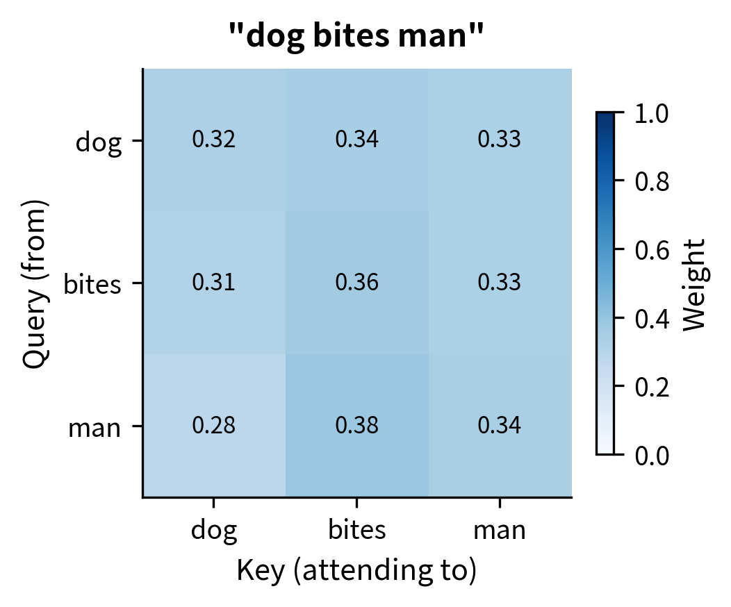
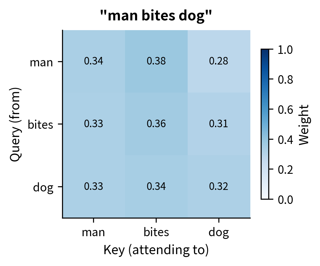
The heatmaps reveal the core problem. Despite "dog bites man" and "man bites dog" having opposite meanings, the attention weight between "dog" and "bites" is identical in both sentences (as shown by matching cell values). Self-attention cannot tell that in one sentence the dog is biting, while in the other the dog is being bitten. The pairwise content relationships are the same; only the positions differ.

Understanding why position matters helps us identify what properties any positional encoding scheme should have. The ideal solution must satisfy several requirements:

• Unique position identification: Each position in a sequence needs a distinct representation. If positions 3 and 7 have identical positional signals, the model cannot distinguish them. This seems obvious, but it rules out trivial solutions like using the same constant everywhere.
• Bounded and stable values: Whatever numerical representation we use for position, it should have bounded, well-behaved values. If position 1 is encoded as 1, position 1000 as 1000, and position 1 million as 1 million, the scale differences will overwhelm the semantic content. Neural networks prefer inputs with similar magnitudes.
• Consistent across sequence lengths: The encoding for position 5 should be similar whether it appears in a 10-token sequence or a 1000-token sequence. If positional representations change dramatically based on sequence length, the model must re-learn positional patterns for every possible length.
• Relative position accessibility: Many linguistic relationships depend on relative rather than absolute position. A verb typically appears near its subject and object, regardless of where they fall in the sentence. Ideally, the positional encoding makes it easy to determine that position 7 is "2 steps after" position 5, not just that they're both somewhere in the sequence.
• Generalization beyond training: Models trained on sequences of length 512 may encounter sequences of length 1024 at inference time. The positional encoding should degrade gracefully (or not at all) when extrapolating to positions not seen during training.
• Compatibility with attention: The positional information must integrate with the attention mechanism in a way that allows position to influence attention patterns. If a query can't distinguish nearby keys from distant keys, positional information isn't flowing into the core computation.

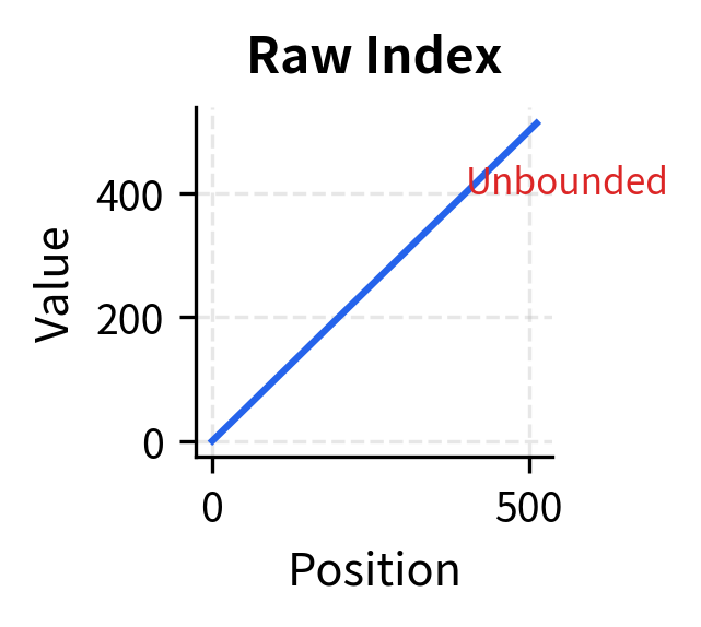
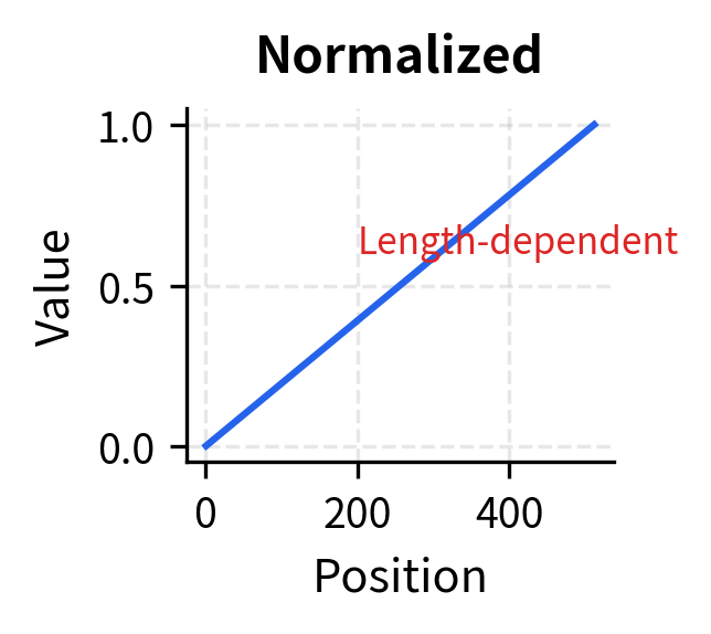
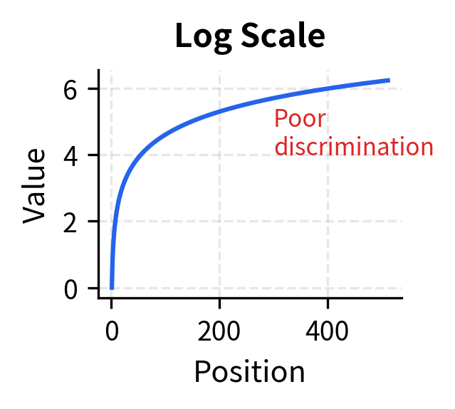
None of these naive approaches satisfy our requirements. Raw indices are unbounded. Normalized positions change meaning with sequence length (position 0.5 is location 256 in a 512-token sequence but location 512 in a 1024-token sequence). Log scaling compresses distant positions so tightly that the model can barely distinguish position 400 from position 500.

Before diving into specific solutions in subsequent chapters, let's clarify an important terminological distinction that often causes confusion.

Positional encoding uses a predetermined formula to compute a position vector. Given position $p$, the encoding function $f(p)$ returns a fixed vector that never changes during training. The classic example is the sinusoidal encoding from the original Transformer paper, which uses sine and cosine functions at different frequencies. The advantage is that the formula generalizes to any position, including positions longer than those seen during training.

Positional embedding treats positions like vocabulary tokens. We create an embedding matrix $P \in \mathbb{R}^{L \times d}$, where $L$ is the maximum sequence length and $d$ is the embedding dimension. Position $p$ simply looks up row $p$ of this matrix, retrieving a $d$-dimensional vector $\mathbf{p}_p$. These embeddings are learned during training, just like word embeddings. The advantage is flexibility: the model can learn whatever positional patterns are useful. The disadvantage is that positions beyond $L$ have no representation.

Most modern language models use positional embeddings (learned lookup tables) rather than fixed encodings, but the terminology often gets mixed. We'll explore both approaches in detail in the following chapters.

Now that we understand the two mechanisms for generating positional vectors, the remaining question is: how do we inject this information into the attention computation? Recall from our earlier analysis that attention weights depend only on query and key vectors, which are projections of the input embeddings. To make attention position-aware, we need to modify what goes into those projections.

The standard approach is elegantly simple: add the positional vector directly to the token embedding, creating a single combined representation that carries both semantic meaning and positional information:

where:

• $\mathbf{x}_i \in \mathbb{R}^d$: the token embedding at position $i$ (carries semantic content)
• $\mathbf{p}_i \in \mathbb{R}^d$: the positional vector for position $i$ (carries positional information)
• $\mathbf{x}'_i \in \mathbb{R}^d$: the combined representation fed to attention
• $d$: the embedding dimension (must be the same for both token and position vectors)

Why addition rather than concatenation or some other combination? Addition preserves the dimensionality: the combined vector has the same size as the original embedding, so existing projection matrices work unchanged. More subtly, addition allows the model to learn how much weight to give positional versus semantic information. If certain dimensions of the positional encoding are consistently ignored by the learned projections, the model effectively down-weights position for those aspects of the representation.

The shapes confirm that adding positional vectors preserves the embedding dimension. Looking at position 0, you can see how each dimension of the combined vector is simply the sum of the corresponding token and position dimensions. The positional vectors are scaled by 0.1 to keep them relatively small compared to the token embeddings, a common practice that prevents positional information from dominating semantic content. The combined representation now carries both semantic content (from the token embedding) and positional context (from the positional vector). When this combined representation is projected into queries, keys, and values, both types of information can influence the attention pattern.

A final conceptual distinction shapes the design space for positional representations: should we encode where each token is in absolute terms, or should we encode how tokens relate to each other in relative terms?

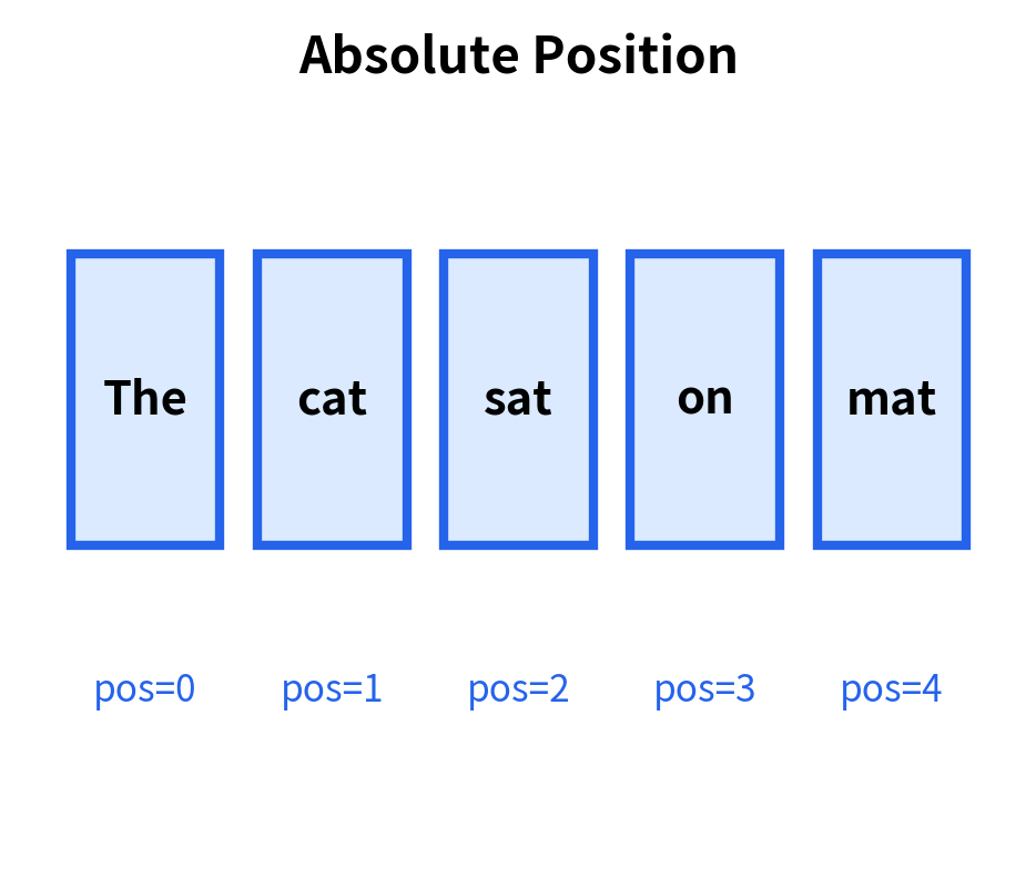
Absolute positional encoding assigns each position a fixed vector. Position 0 always gets the same encoding, position 1 always gets the same encoding, and so on. The attention mechanism must then learn to extract relative information by comparing absolute positions.

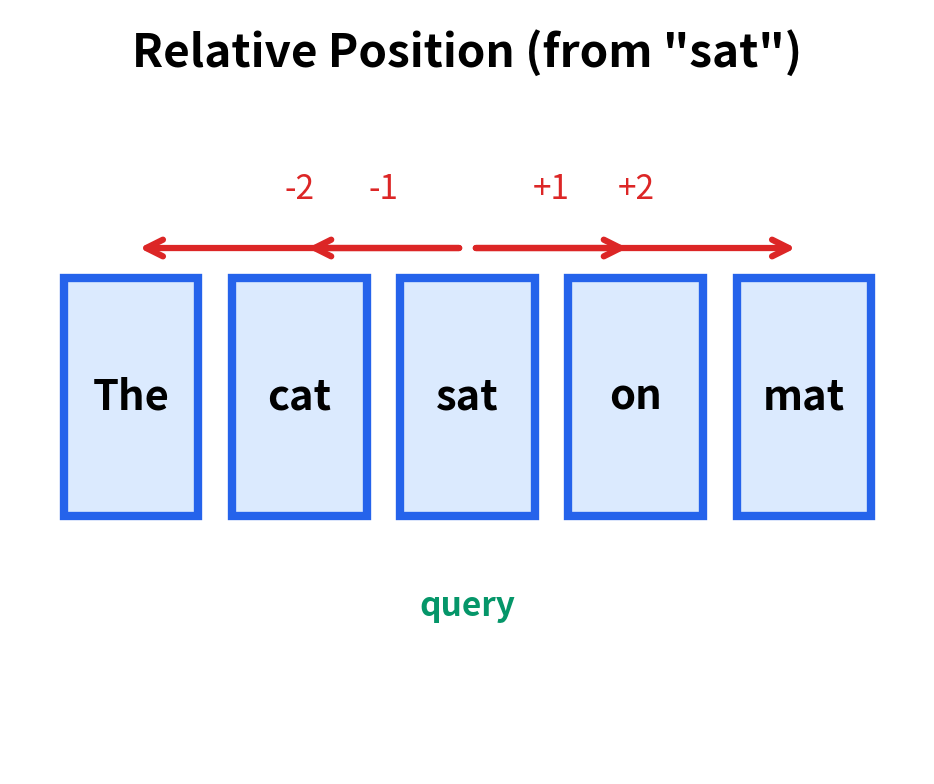
Relative positional encoding directly encodes the distance or relationship between pairs of positions. Instead of saying "this token is at position 5," relative encoding says "this token is 3 positions before the query." The attention mechanism directly incorporates these relative distances.

Each approach has trade-offs. Absolute encoding is simpler to implement: just add a position vector to each token embedding. But linguistic relationships often depend on relative distance. A verb looks for its subject within a few words, regardless of whether they're at positions 3-5 or positions 103-105 in a document. Absolute encoding forces the model to learn this generalization across all possible absolute position pairs.

Relative encoding directly captures these distance-based relationships but requires modifying the attention mechanism itself, not just the input embeddings. The attention score between positions $i$ and $j$ must incorporate information about the distance $i - j$, which complicates the efficient matrix operations we rely on.

Modern architectures increasingly favor relative or hybrid approaches. RoPE (Rotary Position Embedding) cleverly encodes relative positions through rotation operations that integrate naturally with attention. ALiBi (Attention with Linear Biases) adds a simple bias to attention scores based on distance. We'll explore these in dedicated chapters.

No positional encoding scheme is perfect. Every approach makes trade-offs, and understanding these limitations helps choose the right scheme for a given application:

• Fixed encodings may not capture learned patterns. Sinusoidal encoding uses mathematically determined frequencies. These frequencies might not align with the positional patterns most useful for a specific task. A learned embedding can adapt to the training data, potentially discovering better positional representations.
• Learned embeddings don't generalize to longer sequences. If you train with a maximum sequence length of 512, positions 513 and beyond have no learned representation. Some models handle this with interpolation or extrapolation heuristics, but performance often degrades for unseen positions.
• Additive combination limits expressiveness. Adding positional vectors to token embeddings means the combined representation must encode both content and position in a shared space. The model may struggle when positional and semantic information conflict or when fine-grained positional distinctions are needed.
• Relative positions require architectural changes. Directly encoding relative positions requires modifying the attention computation, not just the input. This can complicate implementation and sometimes reduce computational efficiency.
• Very long sequences remain challenging. Even with sophisticated positional encoding, transformers struggle with extremely long sequences (tens of thousands of tokens). The attention mechanism still has quadratic complexity, and positional patterns learned on shorter sequences may not transfer.

Self-attention is blind to position because its computation depends only on content, not on where tokens appear in the sequence. This permutation equivariance is a fundamental property of the attention mechanism, not a bug in any particular implementation.

Key takeaways from this chapter:

• Permutation equivariance: Self-attention produces the same outputs (reordered) regardless of input order. Shuffling the input shuffles the output identically, because attention weights depend only on query-key compatibility, not on position indices.
• Language requires order: Grammatical roles, negation scope, modifier attachment, temporal relationships, and semantic composition all depend on word position. "Dog bites man" and "man bites dog" must be distinguishable.
• Requirements for positional information: Any solution must provide unique position identification, bounded values, consistency across sequence lengths, accessibility of relative positions, generalization beyond training, and compatibility with attention.
• Encoding vs. embedding: Positional encoding uses fixed formulas (like sinusoids) that generalize to any position. Positional embedding uses learned lookup tables that adapt to training data but have fixed maximum length.
• Absolute vs. relative: Absolute encoding assigns fixed vectors to positions. Relative encoding captures distances between positions. Modern architectures increasingly favor relative approaches for better generalization.

In the next chapter, we'll examine the sinusoidal positional encoding introduced in the original Transformer paper. This elegant mathematical construction uses sine and cosine functions at different frequencies to create unique position vectors that support relative position computation through simple linear operations.

Ready to test your understanding? Take this quick quiz to reinforce what you've learned about the position problem in self-attention.