Grouped Query Attention: Memory-Efficient LLM Inference

Multi-Query Attention (MQA) reduces the key-value cache to a single head, slashing memory by a factor equal to the number of attention heads. This aggressive sharing works well for many applications, but it pushes model capacity to its limit. For tasks requiring nuanced multi-step reasoning or tracking multiple independent information streams, that single key-value representation can become a bottleneck. Grouped Query Attention (GQA) offers a middle path: share key-value heads among groups of query heads, trading off between MQA's extreme memory efficiency and Multi-Head Attention's full representational capacity.

This chapter explores GQA in depth. You'll understand why intermediate sharing often outperforms the extremes, learn the mathematical formulation that makes grouped sharing work, implement GQA from scratch, and analyze the quality-efficiency tradeoffs that have made it the default choice for models like LLaMA 2 and Mistral.

Before diving into GQA, let's place it within the broader landscape of attention mechanisms. The key insight is that key-value sharing exists on a spectrum, with Multi-Head Attention (MHA) and Multi-Query Attention (MQA) as the two extremes.

In standard MHA, each of the $h$ query heads has its own dedicated key and value projections. This maximizes representational capacity but requires storing $h$ key-value pairs in the cache during inference. In MQA, all query heads share a single key-value pair, reducing cache size by a factor of $h$ but potentially limiting what information the model can attend to in parallel.

GQA sits between these extremes. With $h$ query heads and $g$ key-value groups (where $1 < g < h$), each group of $h/g$ query heads shares one key-value pair. The memory reduction factor is $h/g$, which can be tuned to balance efficiency and quality.

The numbers tell a clear story. GQA with 8 key-value heads reduces cache size by 8x compared to MHA, a substantial improvement that enables larger batches or longer sequences. At the same time, it retains 8 separate key-value representations instead of collapsing everything to one, preserving the model's ability to attend to multiple distinct aspects of the input.

The effectiveness of GQA stems from an empirical observation about attention head behavior: many attention heads learn similar patterns. Research on trained transformers has shown that heads often cluster into functional groups, with heads in the same cluster attending to similar types of relationships. GQA exploits this redundancy by formalizing the grouping structure.

Consider a model with 32 query heads. In MHA, each head has its own key-value projection, but analysis often reveals that heads 1-4 learn similar positional patterns, heads 5-8 focus on syntactic relationships, and so on. These natural clusters suggest that forcing heads within a cluster to share key-value projections might not significantly impact model quality while providing substantial memory savings.

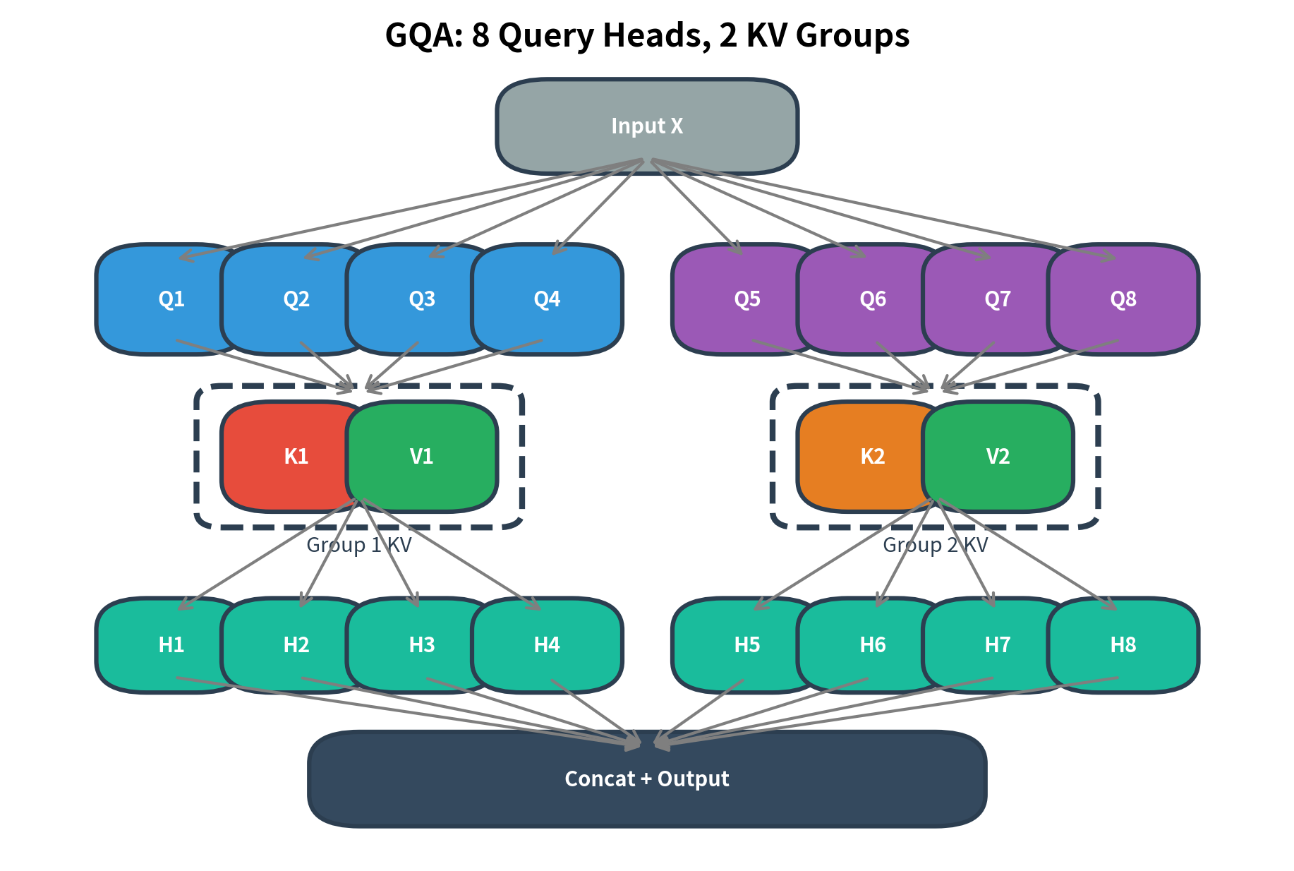
The diagram illustrates GQA with 8 query heads divided into 2 groups. Query heads Q1-Q4 share key-value pair (K1, V1), while Q5-Q8 share (K2, V2). Each group can attend to different aspects of the input through their shared key-value representation, while the queries within each group specialize their attention patterns using different learned projections.

Let's formalize GQA mathematically. The core idea is straightforward: instead of each query head having its own key-value projections (as in MHA) or all query heads sharing one key-value projection (as in MQA), GQA divides query heads into groups where each group shares a single key-value projection.

Given an input sequence $X \in \mathbb{R}^{T \times d}$, GQA is parameterized by:

• $h$: number of query heads (determines query diversity)
• $g$: number of key-value groups, where $g$ divides $h$ evenly (controls memory vs. capacity trade-off)
• $d_k = d / h$: dimension per head (same as standard multi-head attention)

The ratio $h/g$ determines how many query heads share each key-value head. For example, with $h = 32$ query heads and $g = 8$ KV groups, each group of 4 query heads shares one key-value representation.

Query projections work exactly as in standard multi-head attention. Each query head $i$ has its own learned projection matrix that transforms the input into a query representation:

where:

• $Q_i \in \mathbb{R}^{T \times d_k}$: the query matrix for head $i$, containing a $d_k$-dimensional query vector for each of the $T$ positions
• $X \in \mathbb{R}^{T \times d}$: the input sequence with $T$ tokens, each represented as a $d$-dimensional vector
• $W^Q_i \in \mathbb{R}^{d \times d_k}$: the learned query projection matrix for head $i$, transforming from model dimension to head dimension

Having $h$ separate query projections preserves the model's ability to ask $h$ different "questions" of the input. Each query head can still specialize in detecting different patterns, maintaining expressive power.

Here is where GQA diverges from MHA. Instead of $h$ key-value projections, we have only $g$ projections that are shared among groups of query heads:

where:

• $K_j \in \mathbb{R}^{T \times d_k}$: the key matrix for group $j$, containing key vectors for all $T$ positions
• $V_j \in \mathbb{R}^{T \times d_k}$: the value matrix for group $j$, containing value vectors for all $T$ positions
• $W^K_j \in \mathbb{R}^{d \times d_k}$: the learned key projection matrix for group $j$
• $W^V_j \in \mathbb{R}^{d \times d_k}$: the learned value projection matrix for group $j$

With only $g$ key-value projections instead of $h$, the KV cache during inference stores $g$ key-value pairs rather than $h$, reducing memory by a factor of $h/g$.

To connect query heads to their shared key-value representations, we define a grouping function that maps each query head index to its corresponding key-value group:

where:

• $i$: the query head index, ranging from 1 to $h$
• $g$: the total number of key-value groups
• $h$: the total number of query heads
• $\lfloor \cdot \rfloor$: the floor function (rounds down to nearest integer)

This function partitions the $h$ query heads into $g$ groups of size $h/g$ each. For example, with $h = 8$ query heads and $g = 2$ groups:

• Query heads 1, 2, 3, 4 map to group 1 (using $K_1$, $V_1$)
• Query heads 5, 6, 7, 8 map to group 2 (using $K_2$, $V_2$)

Each query head computes attention using its own query but the shared key-value from its group:

where:

• $\text{head}_i \in \mathbb{R}^{T \times d_k}$: the output of attention head $i$
• $Q_i \in \mathbb{R}^{T \times d_k}$: the query matrix for head $i$ (unique to this head)
• $K_{\text{group}(i)} \in \mathbb{R}^{T \times d_k}$: the key matrix shared by all heads in group $\text{group}(i)$
• $V_{\text{group}(i)} \in \mathbb{R}^{T \times d_k}$: the value matrix shared by all heads in group $\text{group}(i)$
• $Q_i K_{\text{group}(i)}^T \in \mathbb{R}^{T \times T}$: the attention score matrix
• $\sqrt{d_k}$: scaling factor to prevent dot products from growing too large

The key insight is that different query heads in the same group can still learn different attention patterns. Even though heads 1-4 all use $K_1$ and $V_1$, their different query projections $Q_1, Q_2, Q_3, Q_4$ produce different attention weights over the same key-value pairs.

Finally, all head outputs are concatenated and projected back to the model dimension:

where:

• $\text{Concat}(\text{head}_1, \ldots, \text{head}_h) \in \mathbb{R}^{T \times (h \cdot d_k)}$: concatenation of all $h$ head outputs along the feature dimension
• $W^O \in \mathbb{R}^{(h \cdot d_k) \times d}$: the output projection matrix
• $\text{GQA}(X) \in \mathbb{R}^{T \times d}$: the final output, matching the input dimension

Since $h \cdot d_k = d$, the concatenated heads have dimension $d$, and $W^O$ projects back to dimension $d$, preserving the input shape for residual connections.

The key implementation detail is the repeat_interleave operation that expands the key-value tensors to match the number of query heads. This creates the grouping structure: consecutive query heads share the same key-value entries. The KV cache stores only the reduced number of key-value heads, providing the memory savings.

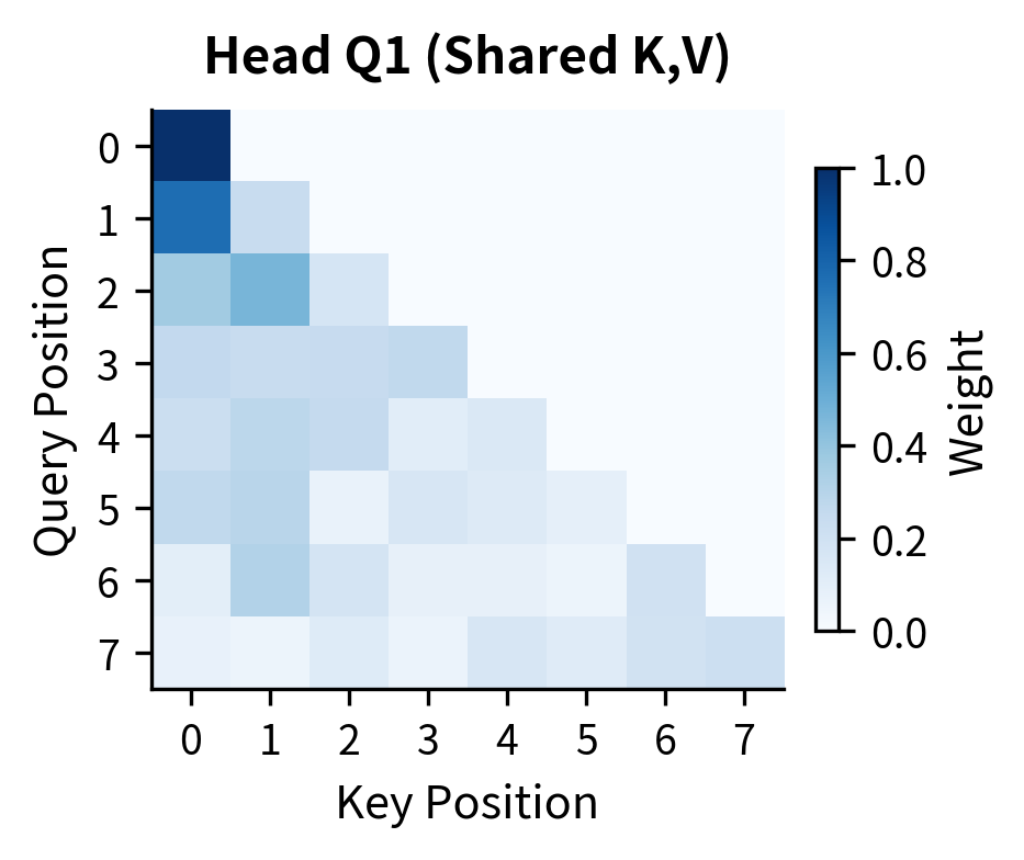
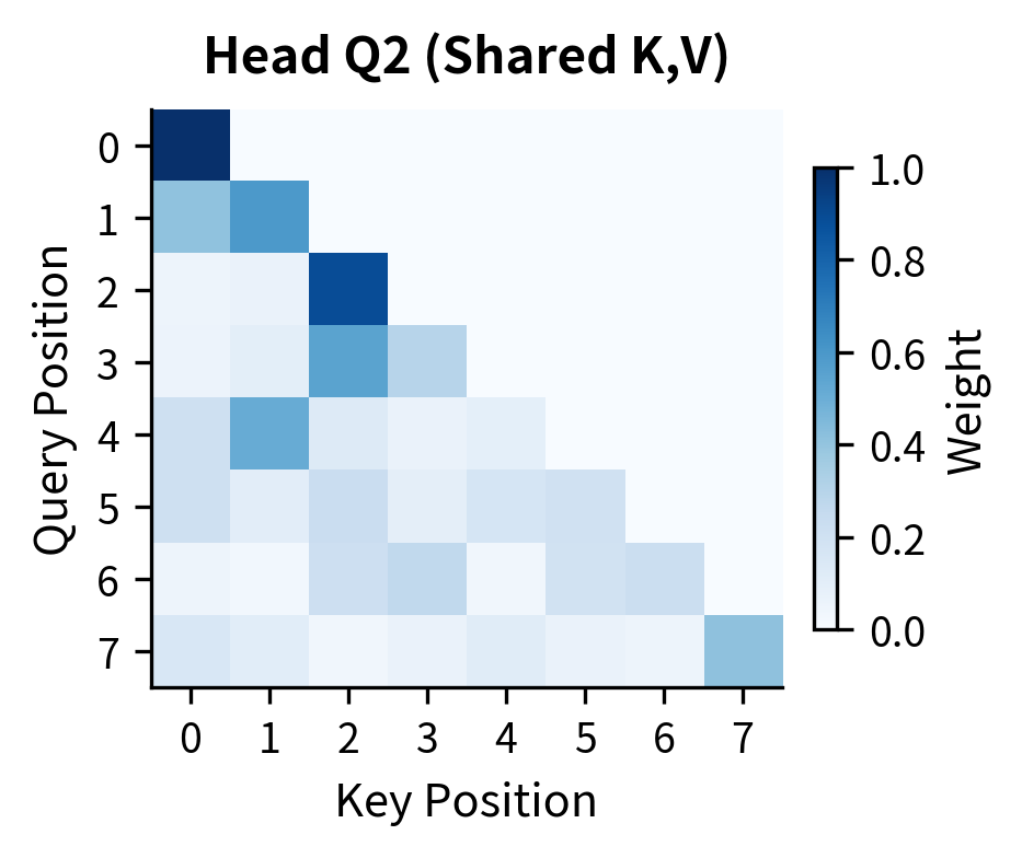
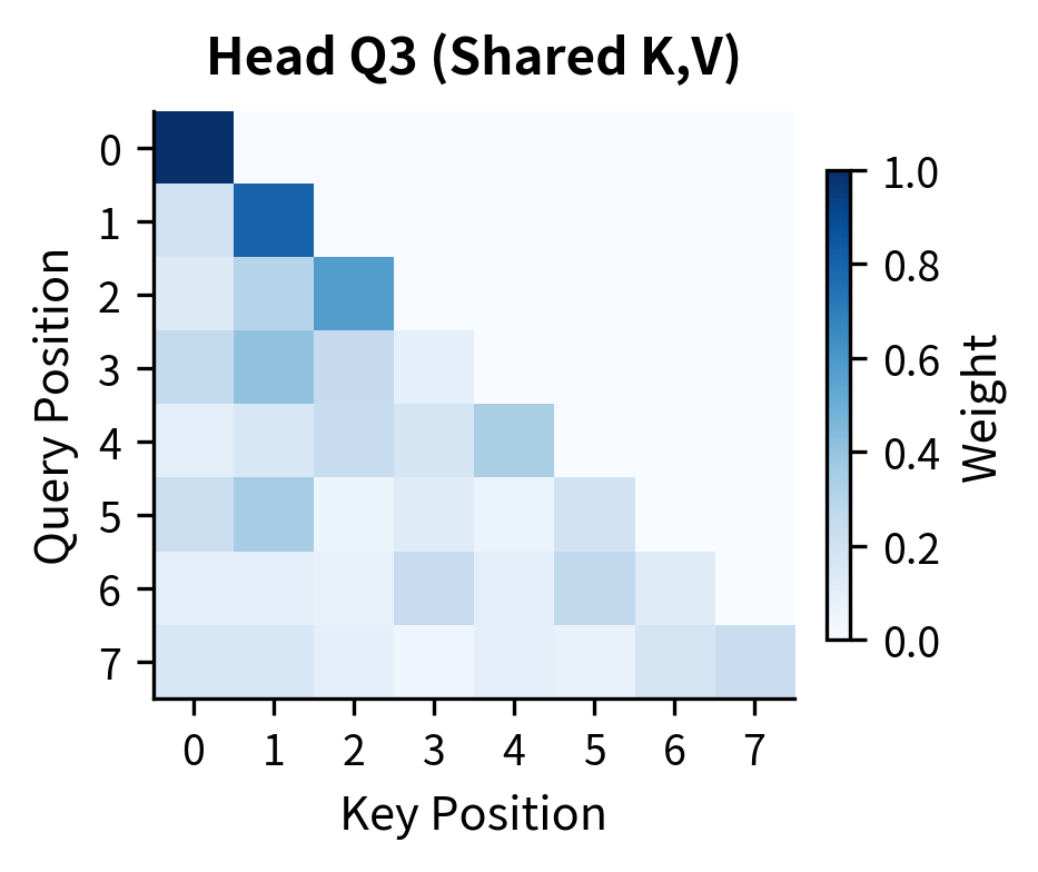
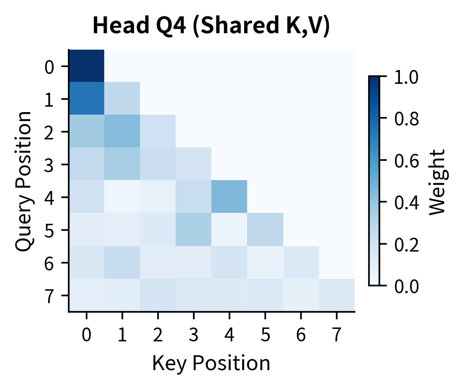
The attention heatmaps above reveal a crucial property of GQA: even though all four query heads share the same key and value tensors (they're all in Group 1), each head produces distinct attention patterns. Head Q1 might focus heavily on recent tokens, Q2 on the first token, Q3 on positions 2-3, and Q4 shows yet another pattern. This diversity emerges because each query head has its own learned projection. The queries are different even when the keys are identical.

The attention heatmaps reveal a crucial property of GQA: even though all four query heads share the same key and value tensors (they're all in Group 1), each head produces distinct attention patterns. Head Q1 might focus heavily on recent tokens, Q2 on the first token, Q3 on positions 2-3, and Q4 shows yet another pattern. This diversity emerges because each query head has its own learned projection. The queries are different even when the keys are identical.

GQA's memory benefits depend on the ratio of query heads to key-value heads. During autoregressive generation, the model caches key and value tensors from previous positions to avoid redundant computation. The size of this KV cache determines how many sequences can be processed in parallel and how long those sequences can be.

For a single transformer layer using GQA, the KV cache stores keys and values for all $g$ groups across all cached positions:

where:

• $2$: accounts for storing both keys and values (two tensors per group)
• $g$: number of key-value groups in GQA
• $d_k$: dimension per head (typically 64 or 128 in modern models)
• $T$: current sequence length (grows during generation)
• $B$: batch size (number of sequences processed in parallel)
• $\text{bytes}$: bytes per element (2 for float16/bfloat16, 4 for float32)

For a full model with $L$ layers, multiply by $L$. The total cache size is $2 \times L \times g \times d_k \times T \times B \times \text{bytes}$.

Comparing GQA to MHA, which stores $h$ key-value heads instead of $g$, the memory reduction is simply the ratio of heads to groups:

where:

• $h$: number of query heads (and number of KV heads in MHA)
• $g$: number of KV groups in GQA

For GQA-8 with 64 query heads, the reduction factor is $64/8 = 8\times$. This means the KV cache is 8 times smaller than it would be with full MHA, enabling either 8 times longer sequences, 8 times larger batches, or some combination of both.

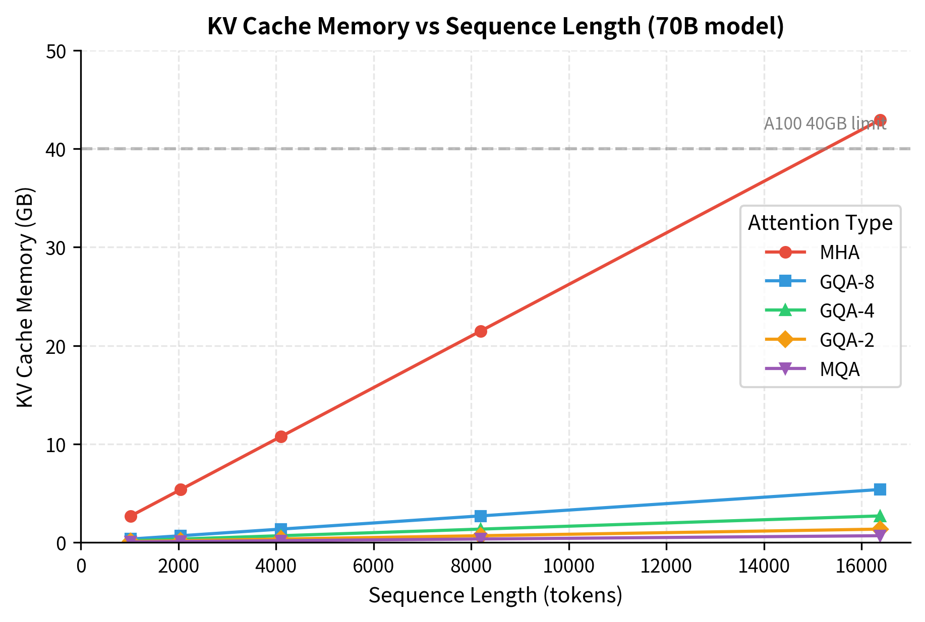
The analysis reveals why GQA-8 has become the standard choice for large models. At 16K tokens, MHA would require 35 GB just for the KV cache, exceeding the memory of most GPUs. GQA-8 reduces this to 4.4 GB, fitting comfortably on modern hardware while retaining 8 independent key-value representations.

Does GQA's additional key-value capacity translate to meaningful quality improvements over MQA? Research from Meta's LLaMA 2 paper and subsequent work provides empirical guidance.

The original GQA paper (Ainslie et al., 2023) conducted extensive experiments comparing MHA, GQA with various group sizes, and MQA. Key findings include:

• GQA with 8 KV heads matches MHA quality within 0.5% on most benchmarks while providing 8x memory reduction
• MQA shows 1-3% quality degradation compared to MHA on complex reasoning tasks
• The quality gap between GQA-8 and MQA is most pronounced on multi-hop reasoning and long-context retrieval

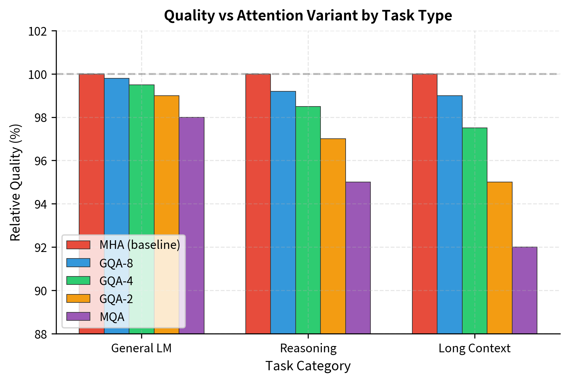
The task breakdown reveals an important pattern. For general language modeling, all variants perform similarly because the task primarily requires local pattern matching. Reasoning tasks show more separation because they require the model to hold multiple pieces of evidence in mind simultaneously. Long-context tasks magnify this effect, as the model must retrieve and combine information from distant positions.

GQA-8 provides the best balance: within 1% of MHA on all tasks while providing substantial memory savings. This explains its adoption in LLaMA 2, Mistral, and other recent models.

For production deployment, efficient KV cache management matters. Let's implement a complete GQA module optimized for autoregressive generation with proper caching.

The cache shape shows (batch, seq, num_kv_heads, head_dim) with only 2 KV heads instead of 8 query heads. During attention, these are expanded via repeat_interleave to match the query head count, but the cache itself remains compact.

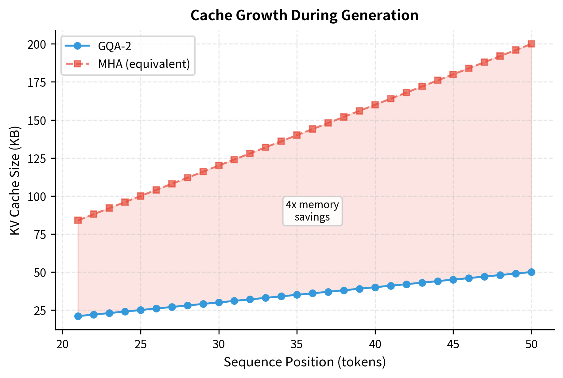
The visualization clearly shows the linear growth of the KV cache during generation. The shaded region represents the memory savings from using GQA-2 instead of MHA. For longer sequences and larger models, these savings become substantial, often determining whether a model fits in GPU memory or requires model parallelism.

The optimal number of KV heads depends on your specific constraints and requirements. Let's develop a framework for making this decision.

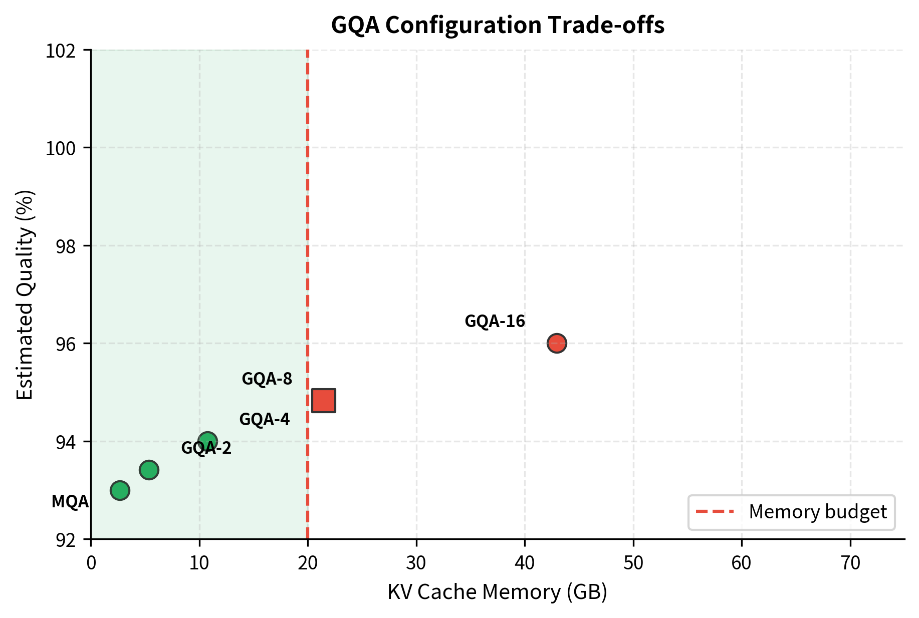
The framework reveals several insights:

• MHA is only viable for small batches or short contexts
• GQA-8 fits most practical deployment scenarios while retaining near-MHA quality
• GQA-4 or GQA-2 may be necessary for very long contexts or large batches
• MQA should be reserved for extreme memory constraints

GQA has become the de facto standard for modern large language models. Here's how major models configure their attention:

A clear pattern emerges: smaller models often retain MHA because memory pressure is manageable, while models at 70B+ scale consistently adopt GQA with 8 key-value heads. This convergence suggests that 8 KV heads represent an empirically validated sweet spot for balancing quality and efficiency at scale.

What if you have an existing MHA model and want the benefits of GQA? The LLaMA 2 paper describes a conversion process called "uptraining" that adapts pretrained MHA models to use GQA.

The conversion process works as follows:

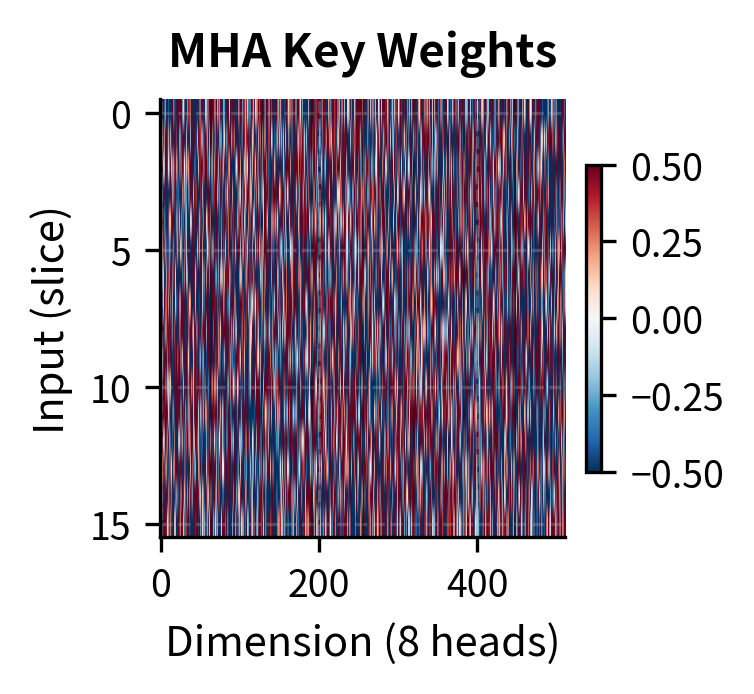
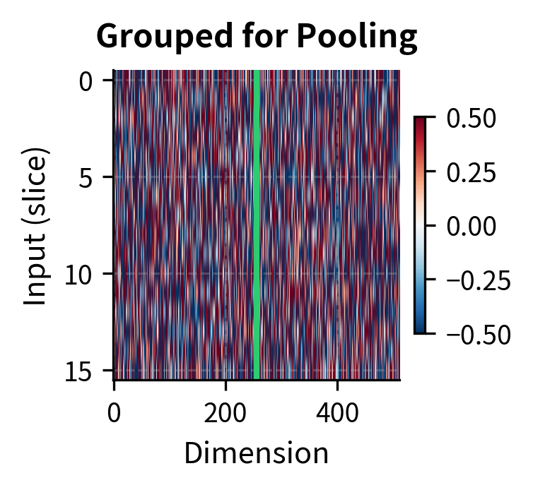
1. Mean pooling: Average the key and value projection weights across the heads that will share a KV representation
2. Uptraining: Continue training the converted model on a small fraction (typically 5%) of the original training data
3. Validation: Verify quality recovery on held-out benchmarks

Mean pooling provides a reasonable initialization, but the converted model typically shows 2-5% quality degradation before uptraining. The uptraining phase allows the model to adapt its query projections to work effectively with the shared key-value representations. Research suggests that 5% of the original training compute is sufficient to recover most of the lost quality.

While GQA provides an excellent balance between efficiency and quality, several practical considerations deserve attention.

The main limitation is inherent to the grouping structure. When multiple query heads share key-value representations, they cannot independently retrieve different information from the context. Consider a task requiring the model to simultaneously track a subject's location and their emotional state. With MHA, separate heads might specialize in these two aspects. With GQA, heads within the same group must coordinate through their queries alone, which may reduce independence. Empirically, this limitation rarely causes problems with 8 KV groups, but becomes more pronounced with fewer groups.

Implementation complexity is slightly higher than MHA. The repeat_interleave operation required to expand KV tensors to match query heads adds overhead and can be tricky to optimize for specific hardware. Modern deep learning frameworks provide efficient implementations, but custom kernels like Flash Attention require explicit GQA support. Most major frameworks now include this, but verify compatibility before deployment.

Debugging attention patterns becomes more challenging with GQA. When visualizing attention weights, remember that heads within a group share the same underlying key-value representation. Patterns that look different may stem entirely from query differences, not from different "views" of the input. This can complicate interpretability analyses.

Finally, the optimal number of KV groups depends on both the model architecture and the target deployment scenario. A model trained with GQA-8 cannot easily be converted to GQA-4 or MQA without quality loss. If you anticipate needing flexibility, consider training multiple variants or designing for the most constrained deployment scenario.

When implementing or configuring GQA, the following parameters have the most significant impact on behavior:

• num_heads (h): The number of query heads. Determines query diversity and must be divisible by num_kv_heads. Common values: 32 (7B models), 64 (70B models). More heads enable more diverse attention patterns but require proportionally more query projection parameters.

• num_kv_heads (g): The number of key-value groups. Controls the memory-quality trade-off. Must divide num_heads evenly. Common values: 8 for large models (GQA-8), 1 for MQA, equal to num_heads for MHA. Lower values reduce KV cache memory but may impact quality on complex reasoning tasks.

• head_dim (d_k): Dimension per attention head, computed as d_model // num_heads. Typical values: 64 or 128. Affects the expressiveness of each attention head and determines the KV cache size per head.

• d_model: Model dimension, must be divisible by num_heads. Standard values: 4096 (7B), 8192 (70B). Larger dimensions increase model capacity but also increase memory requirements.

• Query-to-KV ratio (num_heads // num_kv_heads): Determines how many query heads share each KV head. A ratio of 8:1 (GQA-8) has emerged as the industry standard, providing 8x memory reduction with minimal quality impact.

Grouped Query Attention represents a practical evolution of transformer attention for efficient inference. By sharing key-value heads among groups of query heads, GQA achieves significant memory savings while retaining most of the representational capacity of Multi-Head Attention.

Key takeaways from this chapter:

• GQA groups query heads to share key-value projections, providing a tunable trade-off between MHA's capacity and MQA's efficiency
• Memory savings scale with the ratio of query heads to KV heads: 8 query heads sharing 1 KV head reduces cache by 8x
• Quality impact is minimal for typical ratios: GQA-8 matches MHA within 0.5% on most benchmarks while reducing KV cache by 8x
• 8 KV heads has emerged as the industry standard for large models, used by LLaMA 2 70B, Mistral, Falcon 180B, and others
• Implementation requires expanding KV tensors to match query heads during attention, typically via repeat_interleave
• MHA-to-GQA conversion is possible through mean pooling followed by uptraining on ~5% of training data

The convergence of major model families on GQA-8 suggests this configuration hits an important practical sweet spot. For most large-scale deployments, GQA provides the memory efficiency needed for practical inference without sacrificing the quality that makes the models useful in the first place.

Looking ahead, attention efficiency research continues to evolve. Techniques like sliding window attention, sparse attention, and linear attention offer complementary approaches to managing long sequences. GQA can be combined with these methods, and future chapters will explore how these techniques work together in modern architectures.

Ready to test your understanding? Take this quick quiz to reinforce what you've learned about Grouped Query Attention.