Learned Position Embeddings: Training Transformers to Understand Position

The previous chapter introduced sinusoidal position encoding, a fixed mathematical function that assigns each position a unique pattern. The approach is elegant and principled, with wavelengths designed to enable relative position detection. But there's an alternative philosophy: instead of designing position representations by hand, why not learn them from data?

Learned position embeddings take a different stance. Rather than encoding position through a predetermined formula, they treat position representations as trainable parameters. Just as word embeddings are learned vectors that capture semantic meaning, position embeddings can be learned vectors that capture positional meaning. The model discovers what aspects of position matter for the task at hand.

This approach powers many influential models, including GPT-2, GPT-3, and BERT. Understanding learned position embeddings is essential for working with these architectures and for making informed choices about position encoding in new models.

The core idea is simple: maintain a lookup table of position vectors, one for each position in the sequence. When processing a sequence, look up the embedding for each position and add it to the corresponding token embedding.

Mathematically, if $\mathbf{P} \in \mathbb{R}^{L_{\max} \times d}$ is the position embedding table, then the position embedding for position $i$ is simply:

where:

• $\mathbf{p}_i \in \mathbb{R}^d$: the position embedding vector for position $i$
• $\mathbf{P} \in \mathbb{R}^{L_{\max} \times d}$: the position embedding table (a learnable parameter matrix)
• $L_{\max}$: the maximum sequence length the model can handle
• $d$: the embedding dimension (same as token embeddings)
• $i$: the position index (0-indexed, so $i \in \{0, 1, \ldots, L_{\max} - 1\}$)

This is identical to how word embeddings work: just as we look up a word's embedding from a vocabulary table, we look up a position's embedding from a position table.

The implementation mirrors how word embedding layers work in deep learning frameworks. In PyTorch, you would use nn.Embedding(max_seq_len, embed_dim), which handles the lookup and gradient computation automatically.

Let's create a position embedding table and examine what the initial (random) embeddings look like:

At initialization, the position embeddings are random vectors with no meaningful structure. The magic happens during training, when gradients flow back through these embeddings and reshape them to capture positional patterns useful for the task.

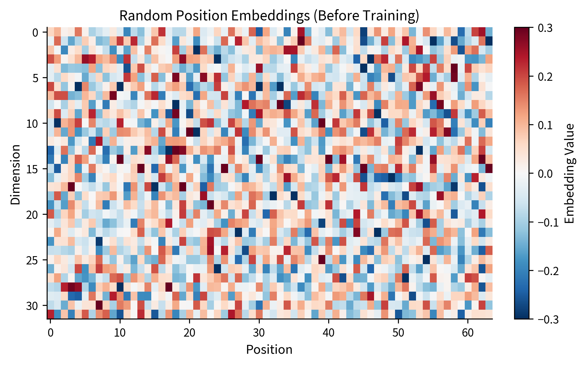
The heatmap reveals the chaotic structure of random initialization. Each column (position) has values that appear unrelated to neighboring columns. There's no smooth gradient, no pattern that would help the model understand that position 5 is closer to position 6 than to position 50. This randomness is the starting point; training will transform this noise into meaningful structure.

Just as with sinusoidal encoding, learned position embeddings are typically added to token embeddings:

where:

• $\mathbf{h}_i \in \mathbb{R}^d$: the input representation for position $i$, combining token and position information
• $\mathbf{e}_{w_i} \in \mathbb{R}^d$: the token embedding for the word at position $i$
• $\mathbf{p}_i \in \mathbb{R}^d$: the position embedding for position $i$

This additive combination means position information is blended into the token representation from the very first layer. The model sees each token as existing at a particular position, not as a position-agnostic entity.

The combined embeddings carry information about both what token appears at each position and where that position is in the sequence. This is the representation that attention layers will operate on.

Position embeddings learn through the same backpropagation process as all other parameters. When the model makes a prediction, gradients flow backward through the network, and the position embeddings receive updates that push them toward configurations that reduce the loss.

But what patterns do position embeddings actually learn? Research has revealed several consistent findings.

Position embeddings typically learn to encode absolute position information directly. Nearby positions tend to have similar embeddings, creating a smooth gradient across the sequence. This makes intuitive sense: positions 5 and 6 are more similar (in terms of their role in the sequence) than positions 5 and 50.

Let's simulate what trained position embeddings might look like by creating a toy example with smoothly varying patterns:

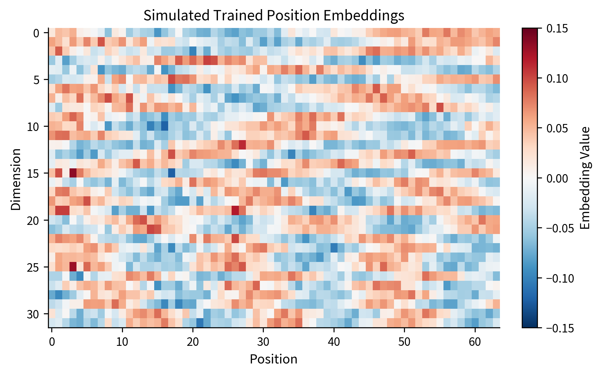
The visualization shows the characteristic structure of learned position embeddings. Different dimensions capture different aspects of position: some vary slowly across the entire sequence (low-frequency components), while others vary more rapidly (high-frequency components). This multi-scale representation allows the model to detect both global position ("near the start vs. near the end") and local structure ("two positions apart").

One way to understand what position embeddings have learned is to compute similarities between positions. If the model uses position for word order and syntax, nearby positions should be more similar than distant ones.

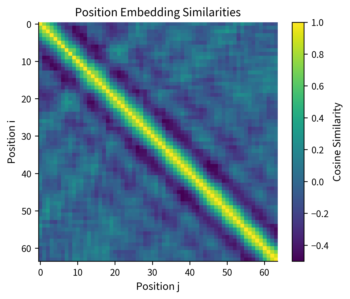
The similarity matrix reveals the structure learned by position embeddings. The bright diagonal indicates that each position is most similar to itself (similarity = 1). The gradual darkening as we move away from the diagonal shows that nearby positions are more similar than distant ones. This band structure is characteristic of well-trained position embeddings.

Let's quantify how similarity decreases with distance:

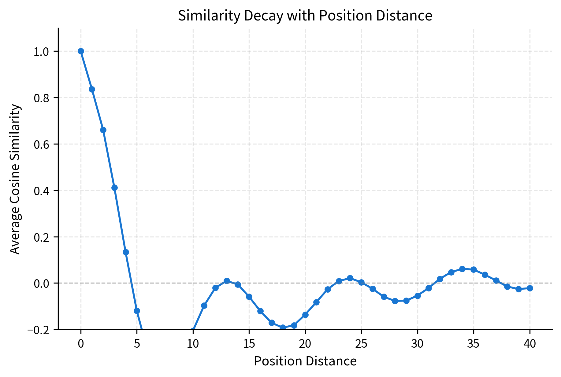
The decay curve shows that similarity drops off smoothly with distance. Positions 1 apart have high similarity (around 0.9), while positions 20+ apart have near-zero similarity. This pattern allows the model to detect relative position through embedding similarity: if two position embeddings are very similar, the positions are likely close together.

Unlike sinusoidal encodings, learned position embeddings have a hard constraint: the model can only handle sequences up to length $L_{\max}$. If you train with $L_{\max} = 512$, you have 512 position embeddings. Position 513 simply doesn't exist in the table.

This creates practical challenges.

During training, you choose $L_{\max}$ based on your computational budget and data characteristics. Larger $L_{\max}$ means more parameters (the position table has $L_{\max} \times d$ values) and higher memory usage during training.

During inference, sequences longer than $L_{\max}$ cannot be processed directly. You must either truncate the sequence, use sliding windows, or fine-tune with a larger $L_{\max}$.

The constraint is fundamental to the approach. Sinusoidal encodings can generate a representation for any position using the formula, but learned embeddings must be stored explicitly. This is a key trade-off between the two approaches.

What happens if you need to process sequences longer than $L_{\max}$? With learned embeddings, you have several options, none of which are ideal.

Option 1: Extend and fine-tune. Add new position embeddings for positions beyond $L_{\max}$, initialize them (perhaps by interpolating from existing embeddings), and fine-tune on longer sequences. This works but requires additional training.

Option 2: Position interpolation. If you trained with $L_{\max} = 512$ but need to handle 1024 tokens, you can interpolate the position indices. Position 512 in the long sequence uses the embedding for position 256 in the original table. This trick, called position interpolation, works surprisingly well for moderate extensions.

Position interpolation effectively "stretches" the position embedding table. The model sees positions at half the resolution, but the relative ordering is preserved. This works because the model primarily cares about relative positions, and those relationships are maintained under scaling.

Let's visualize how position interpolation affects the embedding structure:

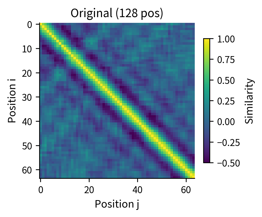
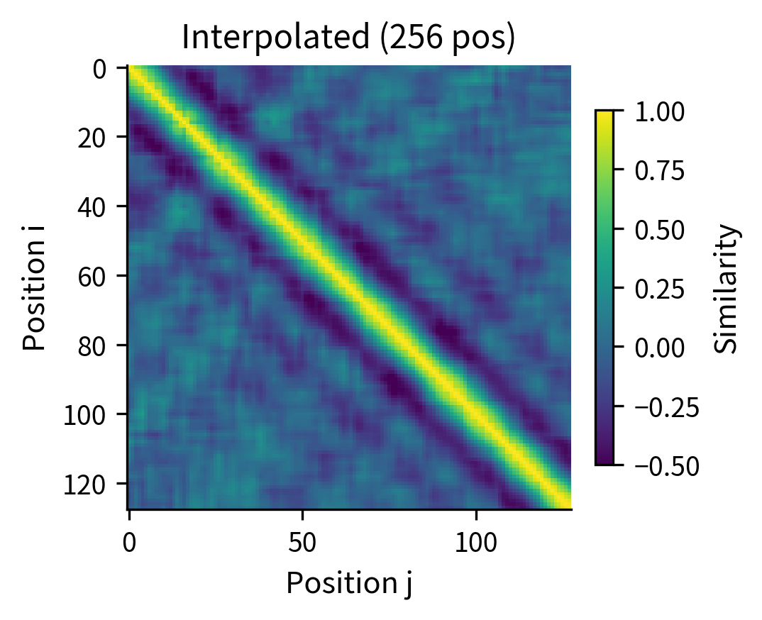
The side-by-side comparison shows that position interpolation preserves the essential structure: nearby positions remain similar, and similarity decays with distance. The interpolated version has twice as many positions, but the relative relationships are maintained. This explains why interpolation works reasonably well for moderate length extensions.

Option 3: Sliding window. Process long sequences in overlapping chunks of length $L_{\max}$. Each chunk gets proper position embeddings, but you need a strategy for combining predictions across chunks. This is common for very long documents.

The extrapolation problem is a significant limitation of learned position embeddings. Models trained with shorter contexts may struggle when forced to process longer sequences, even with interpolation tricks. This has motivated research into position encodings that generalize better, which we'll explore in later chapters.

GPT-2 and GPT-3 use learned position embeddings in a straightforward way. The architecture adds token and position embeddings at the input layer, then processes the combined representation through transformer blocks.

The parameter count reveals an important insight: position embeddings are relatively cheap. In GPT-2 with its 50K vocabulary and 1024 positions, the position embedding table has only 0.79M parameters versus 38.6M for token embeddings. The position table is about 2% of the embedding layer. This makes increasing $L_{\max}$ computationally inexpensive in terms of parameters, though it increases the quadratic attention cost.

BERT also uses learned position embeddings, but with a few differences. BERT includes segment embeddings (to distinguish between sentence pairs) and uses a different initialization scheme.

The addition of segment embeddings allows BERT to understand sentence structure in tasks like next sentence prediction and question answering. The position embeddings work identically to GPT-style: a simple lookup and addition.

When researchers analyze trained position embeddings from models like GPT-2 and BERT, several patterns emerge consistently.

Low-rank structure. The 768-dimensional position embeddings can often be approximated well by a much lower-dimensional subspace. The first 50-100 principal components typically capture most of the variance.

Smooth interpolation. Adjacent positions have similar embeddings, and this similarity decreases smoothly with distance. The embeddings form a continuous manifold in the embedding space.

Boundary effects. The first few positions (0, 1, 2) and positions near $L_{\max}$ sometimes show different patterns, possibly because they're encountered in distinct contexts during training.

Let's visualize the low-rank structure:

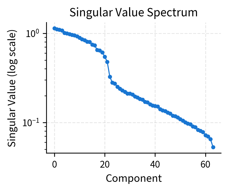
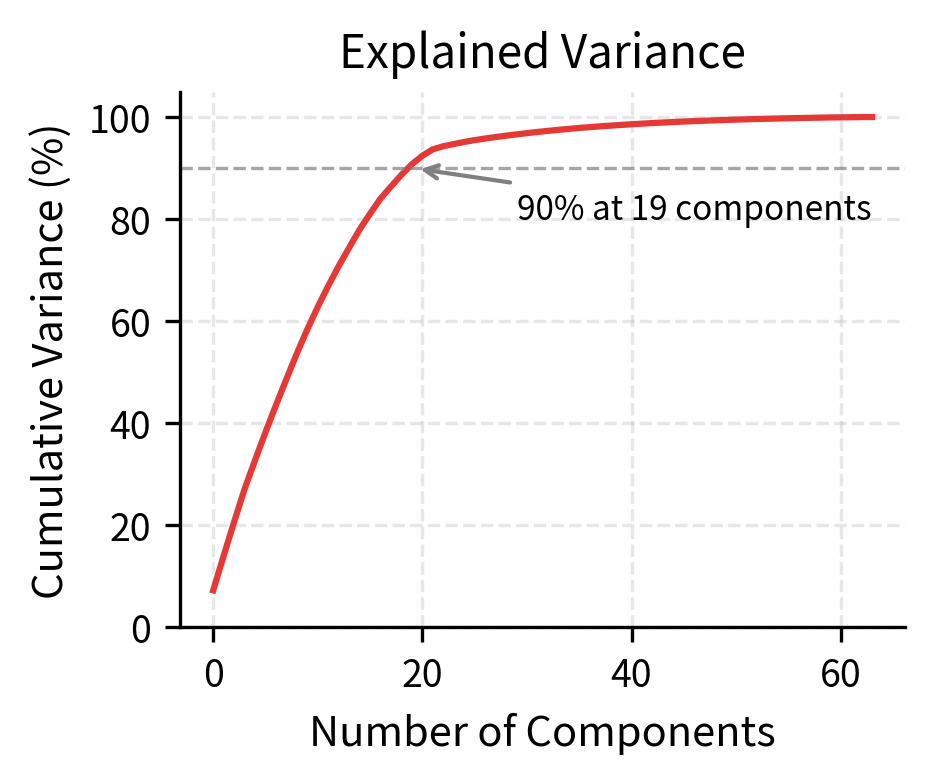
The rapid decay of singular values confirms the low-rank structure. Most of the information in position embeddings can be captured by a handful of principal components. This suggests that positions are fundamentally simple, even though we represent them in high-dimensional space. The extra dimensions provide capacity for task-specific adjustments during training.

The choice between learned and sinusoidal position encodings involves several trade-offs.

Flexibility. Learned embeddings can capture any pattern the data requires, including task-specific positional biases. Sinusoidal encodings impose a fixed mathematical structure that may not match the task's needs. For most NLP tasks, learned embeddings perform as well or better than sinusoidal encodings when the model is trained on sufficient data.

Generalization to longer sequences. Sinusoidal encodings can generate representations for any position, including those never seen during training. Learned embeddings are limited to $L_{\max}$ and may degrade for positions near the boundary where less training signal exists. For applications requiring length generalization, sinusoidal or other fixed encodings have an advantage.

Parameter count. Learned embeddings add $L_{\max} \times d$ parameters. For typical transformer sizes, this is a small fraction of total parameters. Sinusoidal encodings add zero parameters since they're computed from a formula.

Interpretability. Sinusoidal encodings have clear mathematical properties (the dot product encodes relative position, different frequencies capture different scales). Learned embeddings are opaque; their properties must be discovered empirically through analysis.

Training efficiency. Learned embeddings must be trained, which requires gradients to flow through positions encountered during training. Rare positions (e.g., near $L_{\max}$ when most training sequences are short) may receive insufficient updates. Sinusoidal encodings work correctly immediately, with no training needed for the position component.

In practice, most modern language models use learned position embeddings. The flexibility to adapt to task-specific positional patterns outweighs the generalization advantages of fixed encodings for most applications. The sequence length limit is addressed by choosing $L_{\max}$ large enough for the target use case or by using techniques like position interpolation.

In practice, you would implement learned position embeddings using PyTorch's nn.Embedding layer. Here's what a real implementation looks like:

The PyTorch implementation is clean and efficient. The nn.Embedding layer handles the lookup table and gradient computation automatically. Position indices are created on-the-fly based on sequence length, and the same position embeddings are shared across all examples in a batch.

Learned position embeddings represent a pragmatic approach to position encoding. By treating positions as learnable parameters rather than fixed functions, they allow models to discover optimal position representations for their training data. This flexibility has proven valuable across many tasks, from language modeling to machine translation.

The primary limitation is the fixed sequence length. Models cannot process sequences longer than their training length without additional techniques like position interpolation or fine-tuning with extended context. This constraint has driven research into position encodings that generalize better to unseen lengths, including relative position encodings and rotary position embeddings.

Another limitation is the lack of theoretical guarantees about what the embeddings learn. Unlike sinusoidal encodings, which have clear mathematical properties, learned embeddings are empirical objects whose properties must be discovered through analysis. This makes debugging and interpretation more challenging.

Despite these limitations, learned position embeddings remain a dominant choice for transformer architectures. Their simplicity, effectiveness, and ability to adapt to task-specific patterns have made them the default in models like GPT-2, GPT-3, BERT, and many others. The technique demonstrates a broader principle in deep learning: when you have enough data, learned representations often outperform hand-designed ones.

When implementing learned position embeddings, these parameters determine the capacity and behavior of the position encoding:

• max_seq_len ($L_{\max}$): Maximum sequence length the model can handle. This determines the number of rows in the position embedding table. Common values range from 512 (BERT) to 2048+ (modern GPT variants). Larger values increase memory usage linearly but allow processing longer documents without truncation.

• embed_dim ($d$): Dimension of each position embedding vector. Must match the token embedding dimension for additive combination. Typical values range from 256 to 4096 depending on model size. Higher dimensions provide more capacity but increase parameter count proportionally.

• Initialization scale: Position embeddings are typically initialized with small random values, often scaled by $1/\sqrt{d}$ or using a fixed standard deviation (e.g., 0.02 in GPT-2). Smaller initialization helps training stability by keeping initial representations in a reasonable range.

• dropout: Dropout rate applied after combining token and position embeddings. Values of 0.1 are common. This regularizes the model by randomly zeroing embedding dimensions during training.

The ratio of position parameters to total model parameters is typically small (around 2% for GPT-2), making $L_{\max}$ relatively cheap to increase from a parameter perspective. However, attention complexity scales quadratically with sequence length, which is often the practical bottleneck.

Learned position embeddings treat position representations as trainable parameters rather than fixed formulas. This simple idea has proven remarkably effective across many language modeling tasks.

Key takeaways from this chapter:

• Position embedding table: A learnable matrix of shape $(L_{\max}, d)$ stores one embedding vector per position. Position $i$ is represented by the $i$-th row of this table.

• Additive combination: Position embeddings are added to token embeddings at the input layer, creating representations that encode both what token appears and where it appears.

• Training discovers structure: Through backpropagation, position embeddings learn to encode positional information useful for the task. Nearby positions typically develop similar embeddings.

• Maximum sequence length constraint: Unlike sinusoidal encodings, learned embeddings cannot represent positions beyond $L_{\max}$. Processing longer sequences requires techniques like position interpolation or fine-tuning.

• Low effective dimensionality: Despite being stored in high-dimensional space, position embeddings often lie in a low-rank subspace. A few principal components capture most of the positional information.

• GPT and BERT style: Major models like GPT-2 and BERT use learned position embeddings with simple additive combination. The approach is straightforward to implement and works well in practice.

• Trade-offs vs. sinusoidal: Learned embeddings offer more flexibility but limited length generalization. Sinusoidal encodings generalize to any length but impose fixed structure. The choice depends on the application's requirements.

In the next chapter, we'll explore relative position encodings, which address the extrapolation problem by encoding the distance between positions rather than their absolute locations.

Test your understanding of learned position embeddings and how they differ from fixed encoding schemes.