

Compare transformer position encoding methods including sinusoidal, learned embeddings, RoPE, and ALiBi. Learn trade-offs for extrapolation, efficiency, and implementation.

This article is part of the free-to-read Language AI Handbook
Choose your expertise level to adjust how many terms are explained. Beginners see more tooltips, experts see fewer to maintain reading flow. Hover over underlined terms for instant definitions.
Position Encoding Comparison
We've now explored five distinct approaches to injecting positional information into transformers: sinusoidal encoding, learned embeddings, relative position encoding, Rotary Position Embedding (RoPE), and Attention with Linear Biases (ALiBi). Each method emerged from different design philosophies and makes different trade-offs. This chapter brings everything together, comparing these methods across the dimensions that matter for real-world deployment: extrapolation to longer sequences, training efficiency, implementation complexity, and practical performance.
Understanding these trade-offs is essential for choosing the right positional encoding for your application. A model that must handle variable-length documents needs different properties than one trained on fixed-length contexts. A research prototype has different complexity constraints than a production system serving millions of requests. By the end of this chapter, you'll have a clear framework for making these decisions.
The Core Trade-offs
Before diving into specific comparisons, let's establish the fundamental trade-offs that shape position encoding design. Every method navigates tensions between competing goals.
Position encoding methods generally trade off between three properties: (1) extrapolation to unseen sequence lengths, (2) training efficiency and simplicity, and (3) expressive power for capturing complex positional patterns. No single method excels at all three simultaneously.
Extrapolation vs. expressiveness. Fixed formulas like sinusoidal encoding and ALiBi generalize naturally to any sequence length because they don't depend on learned parameters for specific positions. But this generality comes at a cost: the model can't learn task-specific positional patterns that might improve performance. Learned embeddings can capture subtle positional relationships, but they have no representation for positions beyond their training distribution.
Simplicity vs. flexibility. Adding position vectors to embeddings (as in sinusoidal and learned approaches) is simple to implement and understand. But this additive combination limits how position can influence attention. Methods like RoPE and relative position encoding integrate more deeply with the attention mechanism, providing greater flexibility at the cost of implementation complexity.
Absolute vs. relative information. Absolute encodings provide unique identifiers for each position, making it easy to locate specific tokens. Relative encodings directly capture distances between tokens, which often matters more for linguistic relationships. Hybrid approaches like RoPE encode absolute positions but expose relative information naturally through their mathematical structure.
Extrapolation Benchmarks
The most visible difference between position encoding methods appears when models encounter sequences longer than their training length. This scenario is increasingly common: models trained on 2K or 4K context windows must often process documents with 8K, 16K, or even longer sequences. How gracefully does each method handle this extrapolation?
Setting Up the Comparison
We'll simulate extrapolation by creating position encodings for a sequence twice as long as the "training" length and observing how the representations behave at unseen positions.
Let's implement each position encoding method and examine its behavior at extrapolated positions.
Measuring Representation Quality at Extrapolated Positions
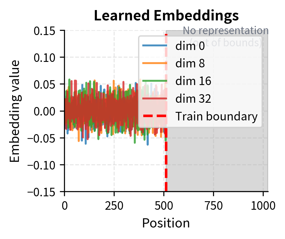
For sinusoidal encoding, extrapolation is mathematically guaranteed to work because the formula applies to any position. For learned embeddings, we have no representation at all for unseen positions. For RoPE, the rotation angles continue following the same pattern. For ALiBi, the linear bias extends naturally.
Before examining extrapolation, let's visualize how each method structures position information across the embedding dimensions. These heatmaps reveal the fundamental patterns each method uses to encode position.
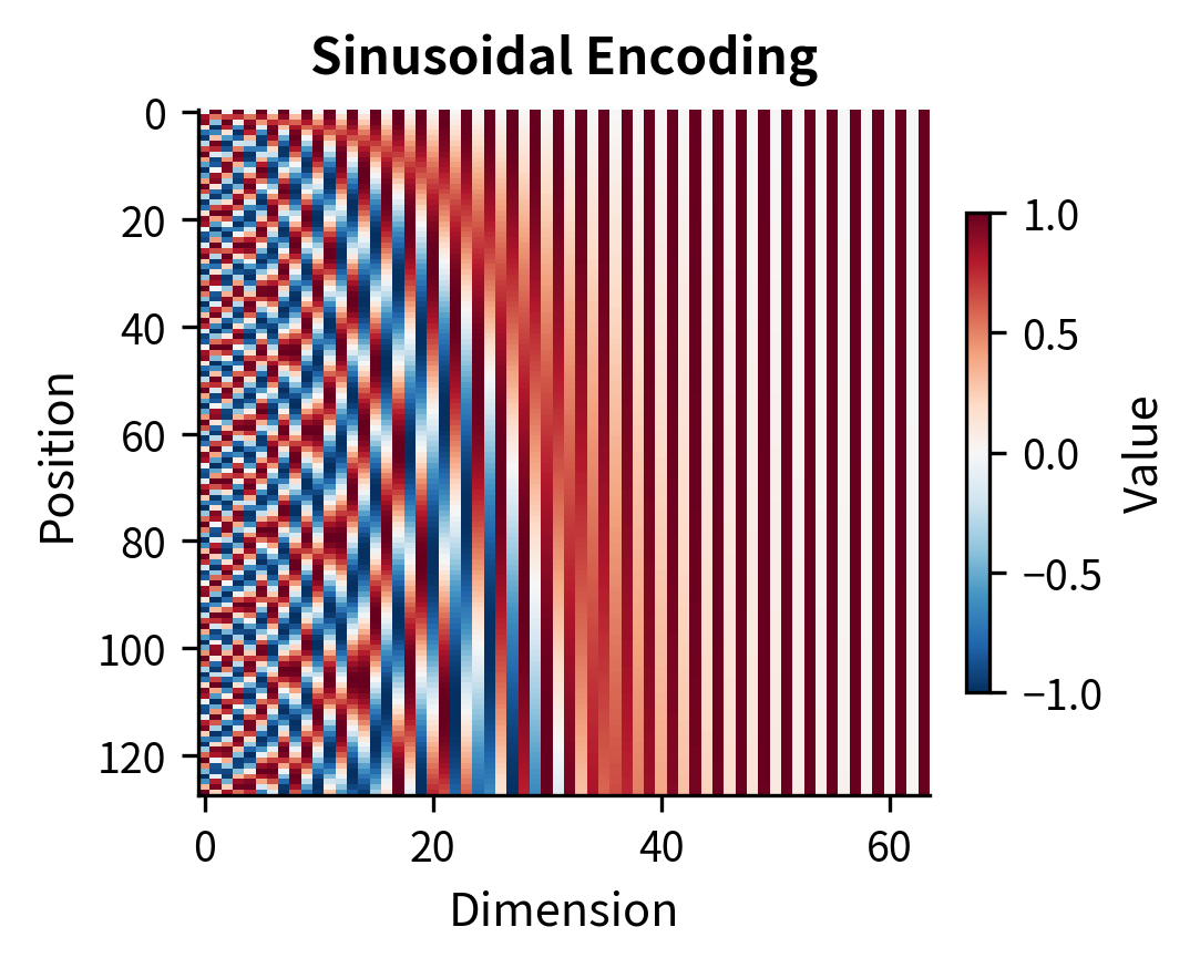
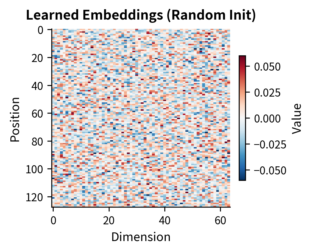
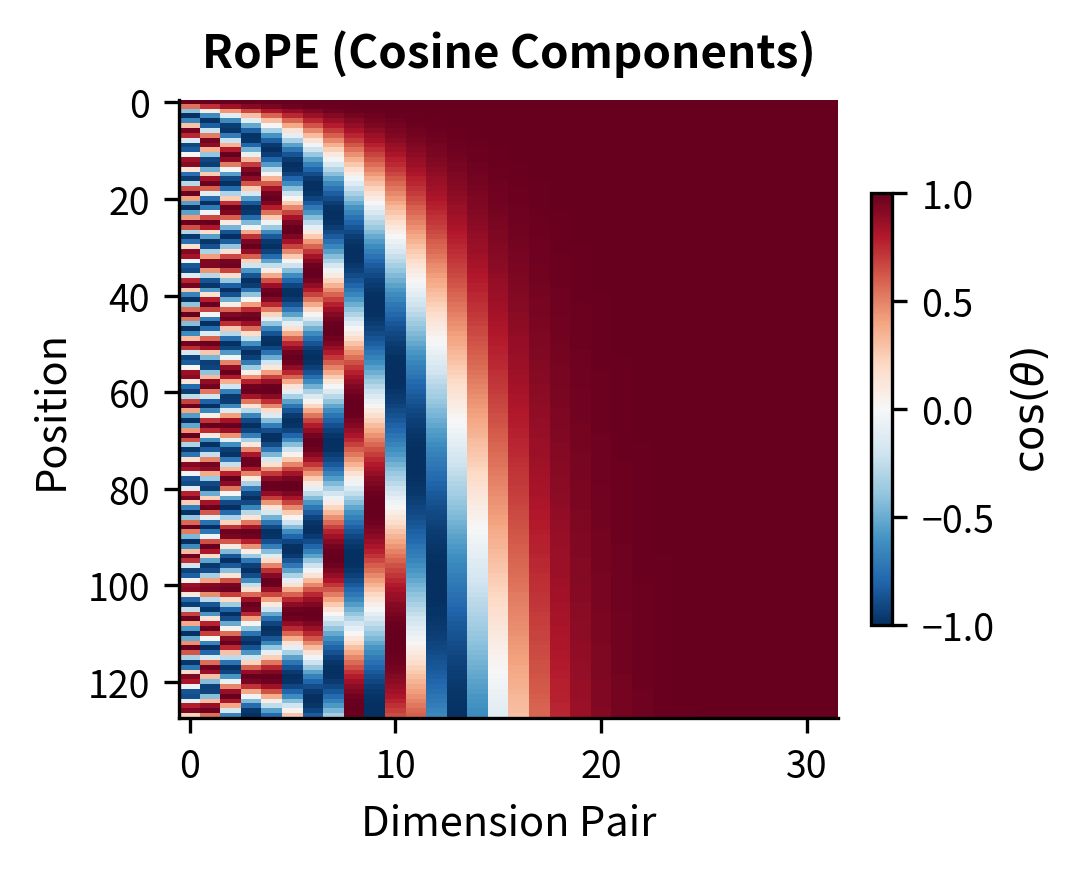
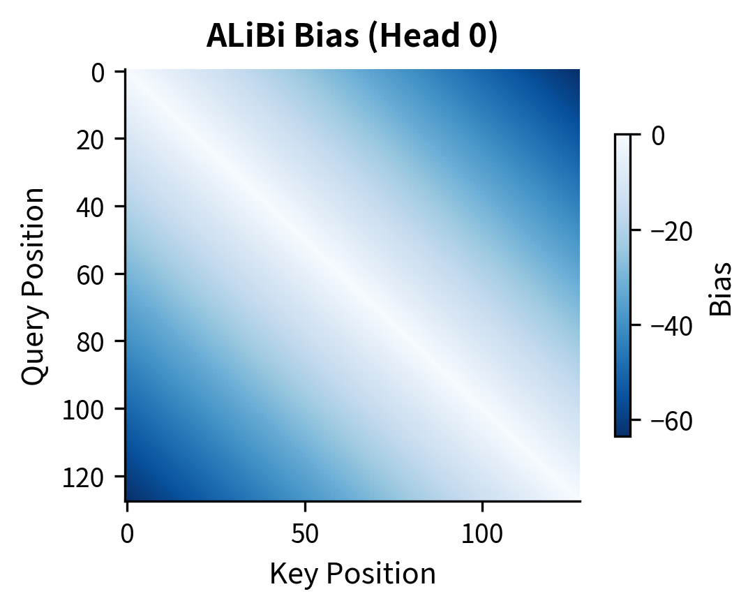
The heatmaps reveal fundamental differences in how each method encodes position. Sinusoidal and RoPE show structured wave patterns with different frequencies across dimensions, enabling the model to capture both fine-grained (nearby positions) and coarse (distant positions) relationships. Learned embeddings start as random noise and must discover useful structure during training. ALiBi operates in a different space entirely, showing the triangular bias pattern that penalizes attention to distant keys.
Let's visualize how each method's representations look at both trained and extrapolated positions.
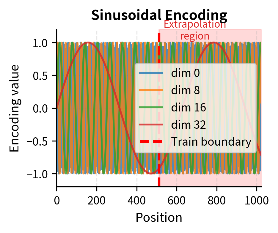
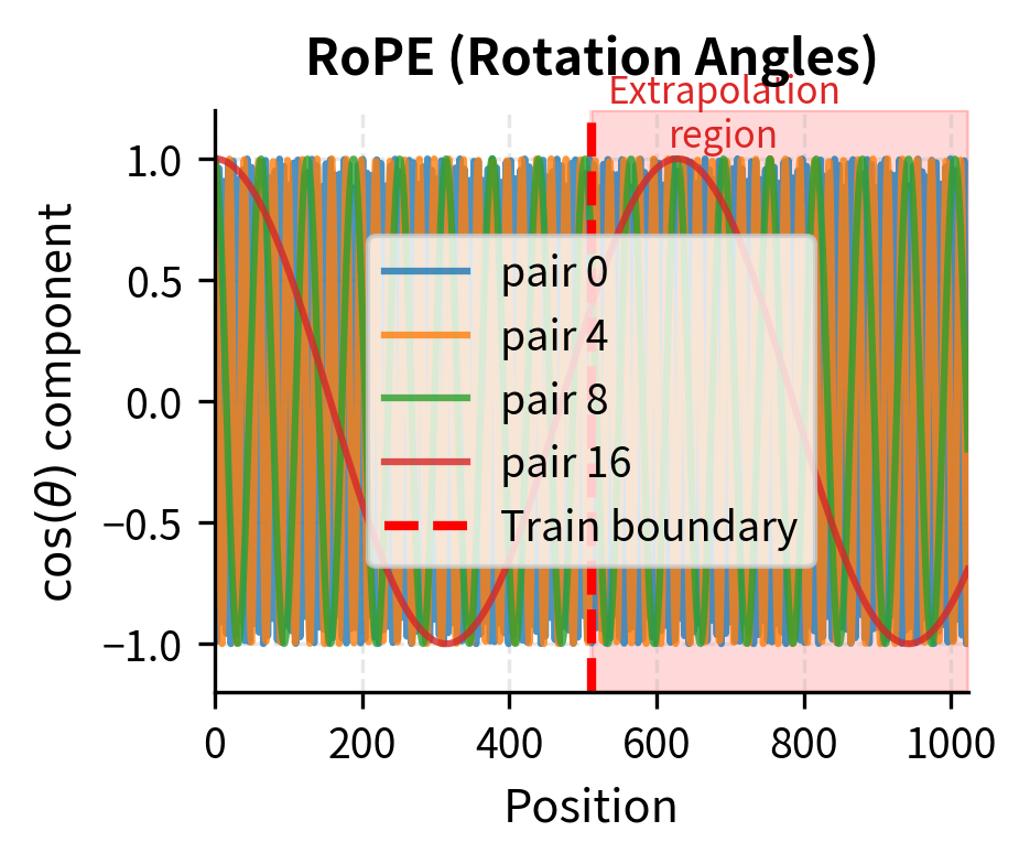
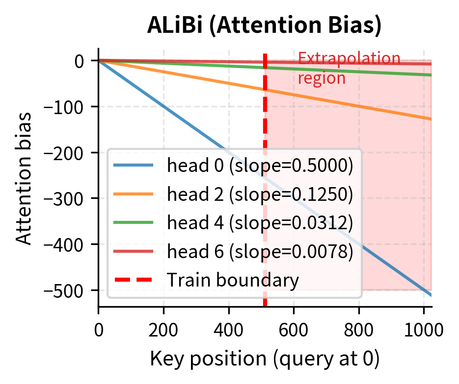
The extrapolation behavior differs dramatically between methods. Sinusoidal encoding continues its periodic patterns seamlessly into the extrapolation region, with each frequency component oscillating according to its fixed formula. RoPE shows the same behavior: rotation angles continue according to the same exponentially-decaying frequency schedule. ALiBi's linear bias grows predictably, applying stronger penalties to more distant positions regardless of whether those distances were seen during training.
Learned embeddings, however, have a fundamental problem: they simply don't exist for unseen positions. The gray region in the plot represents a complete absence of positional information. Various workarounds exist (position interpolation, extrapolation via linear projection), but none match the clean mathematical extension of formula-based methods.
Quantifying Extrapolation Quality
Beyond visual inspection, we can measure extrapolation quality by examining whether the relative position relationships remain consistent. Good extrapolation should preserve the property that nearby positions have similar representations and that relative distances remain meaningful.
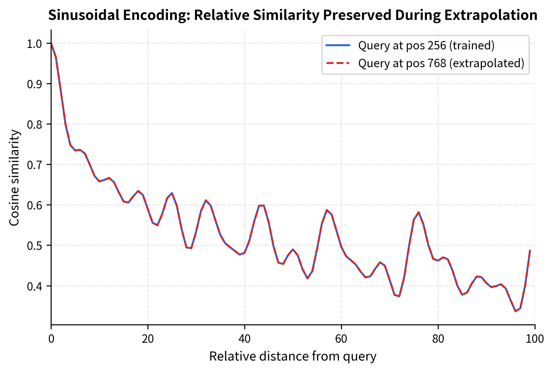
The nearly identical curves demonstrate a crucial property: sinusoidal encoding preserves relative position relationships during extrapolation. Position 768 "looks at" its neighbors in the same way that position 256 does. This consistency is what allows models with sinusoidal or RoPE encoding to generalize, with appropriate scaling adjustments, to longer sequences.
Position Similarity Matrices
Another way to understand position encoding quality is through pairwise similarity matrices. These show how similar any two positions are in the encoding space, revealing whether relative relationships are preserved.
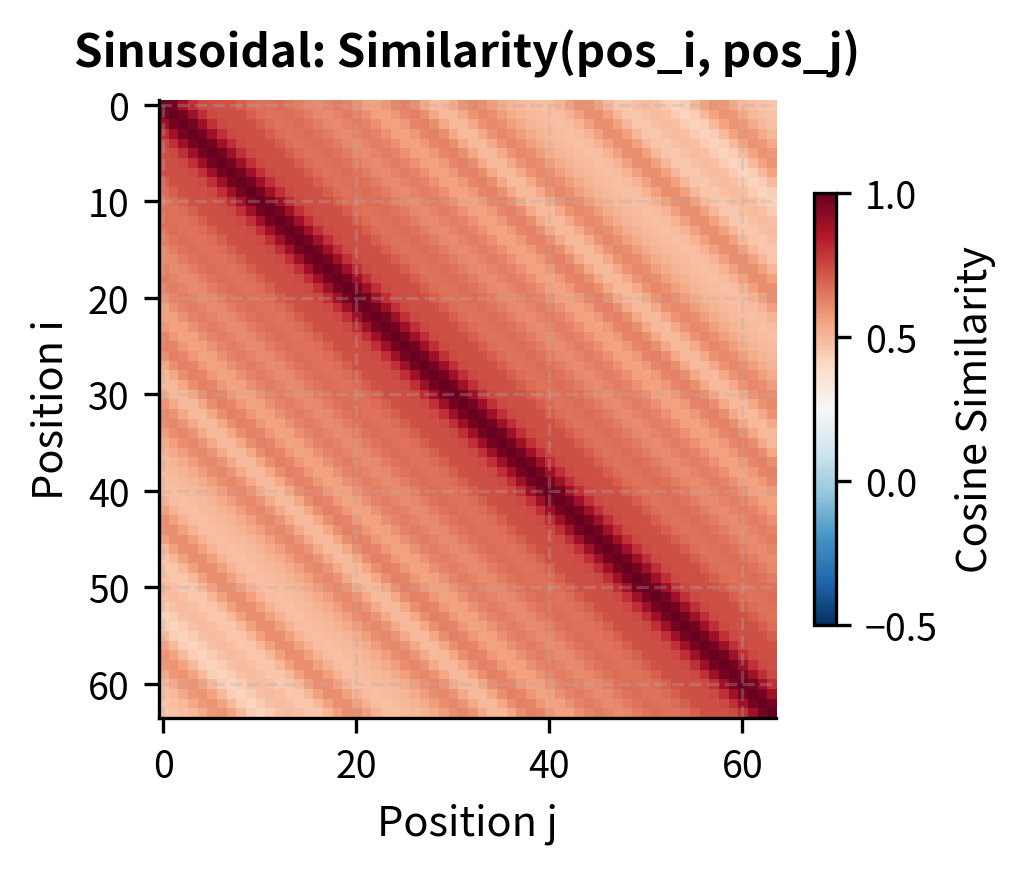
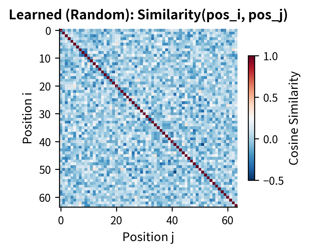
The sinusoidal similarity matrix displays the characteristic banded structure where similarity depends on the relative distance between positions, not their absolute values. This Toeplitz-like property (constant values along diagonals) is what enables position-invariant pattern learning. The learned embeddings, in contrast, show near-zero similarity everywhere except the diagonal, reflecting their random initialization. During training, learned embeddings would develop task-specific similarity structure.
Training Efficiency Comparison
Position encoding choice affects more than just inference behavior. Different methods have different computational costs during training and may require different amounts of data to learn effective representations.
Parameter Counts
The first distinction is the number of parameters each method adds to the model.
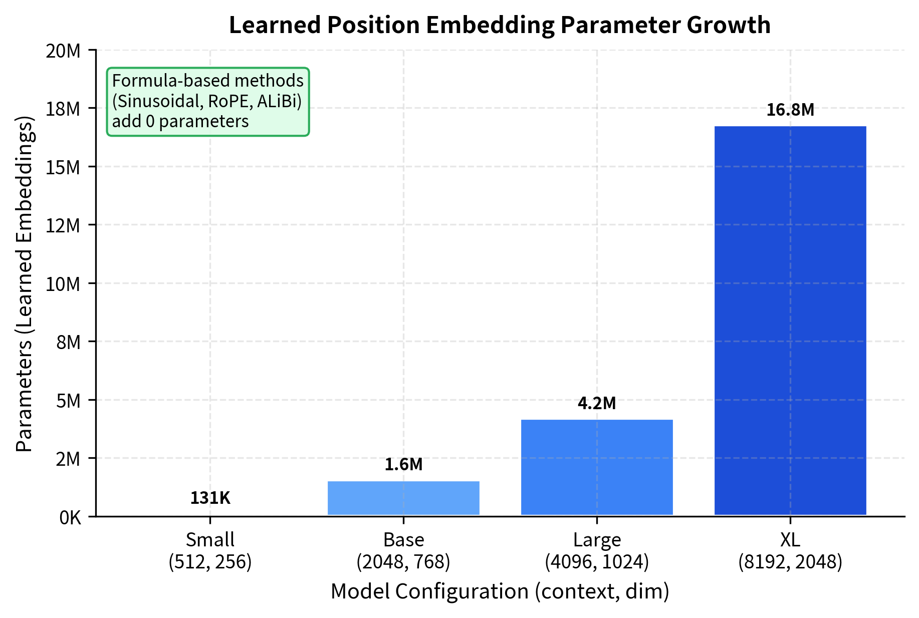
Parameter-free methods like sinusoidal, RoPE, and ALiBi add no trainable weights to the model. This has practical implications beyond memory usage. More parameters mean more opportunities for overfitting, especially when training data is limited. And as context lengths grow, learned embeddings consume an increasing fraction of the model's parameter budget: for a model with 8K context and 2048 dimensions, position embeddings alone require 16 million parameters.
Computational Overhead
Beyond parameters, each method has different computational costs per forward pass.
For a typical configuration (sequence length 2048, key dimension 64), the estimated FLOPs per token differ significantly:
The relative position encoding (Shaw et al.) has higher overhead because it requires additional matrix operations within the attention computation. RoPE's rotations add modest cost but can be fused with existing operations. ALiBi's bias addition is extremely cheap. For most practical purposes, the computational differences between sinusoidal, learned, RoPE, and ALiBi are negligible compared to the attention computation itself.
Training Dynamics
A less quantifiable but important consideration is how quickly each method enables effective learning. Learned embeddings must discover position representations from scratch, while formula-based methods provide structured patterns that may help or hinder learning depending on the task.
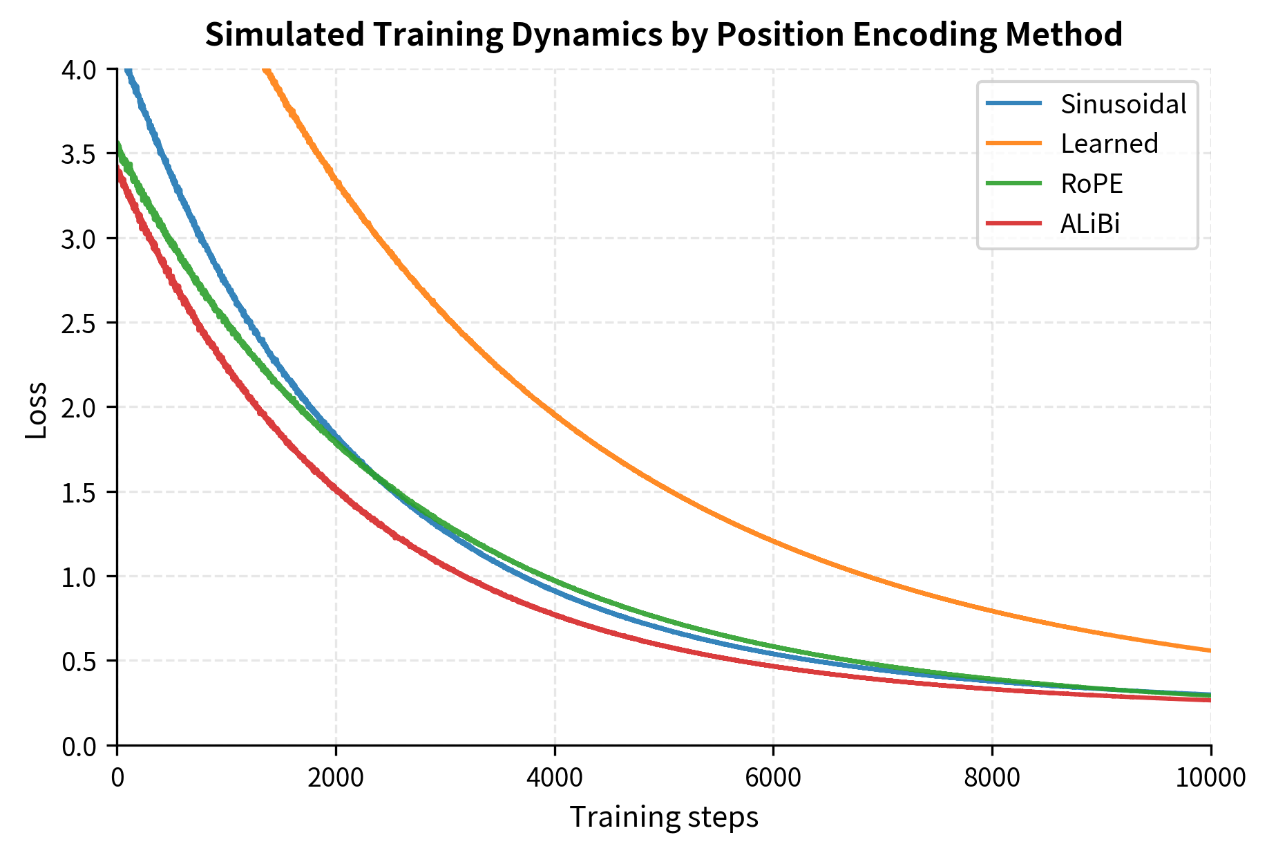
This simulation illustrates a commonly observed pattern: learned embeddings require more training to reach good performance because they start from random initialization. Methods with built-in structure (sinusoidal, RoPE, ALiBi) provide useful inductive biases from the start. The gap typically closes with sufficient training, and learned embeddings sometimes achieve lower final loss because they can adapt to task-specific patterns.
Implementation Complexity
Practical engineering considerations often drive architecture choices as much as theoretical properties. Let's examine the implementation complexity of each method.
Code Complexity Comparison
We'll implement the core logic of each method and compare their complexity.
Let's see these in the context of a complete attention forward pass.
| Method | Where Applied | Modifications Needed | Complexity |
|---|---|---|---|
| Sinusoidal | Input embeddings | Add to embeddings before attention | Simple |
| Learned | Input embeddings | Add to embeddings before attention | Simple |
| Relative (Shaw) | Attention scores | New terms in QK computation | Complex |
| RoPE | Q and K vectors | Rotate Q, K before score computation | Moderate |
| ALiBi | Attention scores | Add bias after score computation | Simple |
The key insight is where each method injects positional information:
- Sinusoidal and Learned: Modify only the input, leaving the attention mechanism untouched
- ALiBi: Adds a bias after scores are computed but before softmax
- RoPE: Transforms Q and K before they interact
- Relative (Shaw): Requires additional terms in the attention score computation
For engineering teams, simpler integration points mean easier maintenance, debugging, and optimization. Methods that modify input embeddings work with any attention implementation. Methods that modify attention internals require careful coordination with optimizations like flash attention.
Position Encoding for Long Context
As language models tackle increasingly long documents, position encoding becomes a bottleneck. Training on 2K tokens and inferring on 100K tokens requires extrapolation strategies that differ by method.
Context Length Scaling Strategies
Each position encoding method has different options for extending context length beyond training.
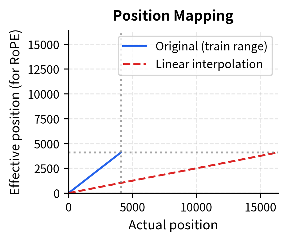
Different models use different extension strategies:
- Linear position interpolation (used in Code Llama): Scales all positions by the extension factor, so position 8192 in an 8K→16K extension becomes effective position 4096
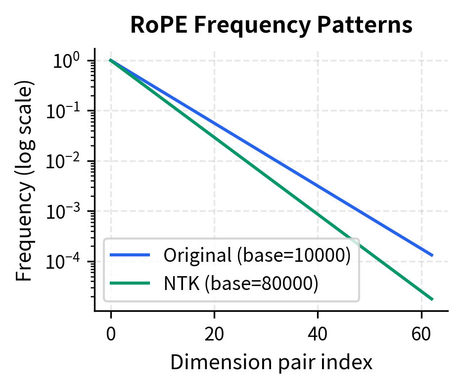
- NTK-aware interpolation: Modifies the frequency base, preserving high-frequency patterns better
- YaRN (Yet another RoPE extension): Combines both approaches with frequency-dependent scaling
- ALiBi: Naturally extends because the linear bias formula applies to any distance
Comparing Long-Context Performance
Let's simulate how well each method maintains coherent attention patterns at extended context lengths.
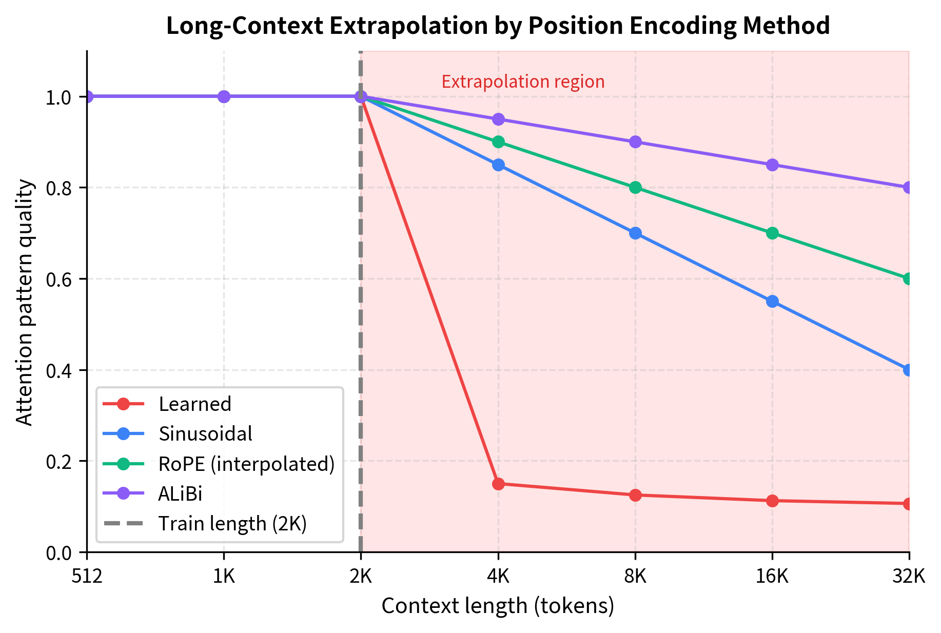
The simulation reflects patterns observed in practice. ALiBi was specifically designed for length extrapolation, and its simple linear penalty on distance generalizes naturally. RoPE with appropriate interpolation techniques can extend well beyond training length, though some quality degradation occurs. Sinusoidal encoding extrapolates mathematically but may not maintain the attention patterns the model learned during training. Learned embeddings fail catastrophically beyond their defined range.
Hybrid Approaches
Real-world architectures increasingly combine multiple position encoding strategies to leverage their complementary strengths.
Common Hybrid Patterns
Several hybrid approaches have emerged in practice:
-
RoPE + ALiBi: Some models apply RoPE to encode relative positions in the query-key interaction while adding an ALiBi-style bias to provide explicit distance penalties. The rotation captures complex relative patterns while the bias ensures distant tokens receive appropriately lower attention.
-
Learned + Sinusoidal: Early experiments in the original Transformer paper found that learned embeddings performed comparably to sinusoidal, leading some models to use sinusoidal initialization with learned fine-tuning. This provides a structured starting point while allowing task-specific adaptation.
-
Block-wise Position Encoding: For very long sequences, some models use local position encoding within blocks and global position encoding across blocks. Tokens have precise position information relative to their local context and coarser information about their position in the document.
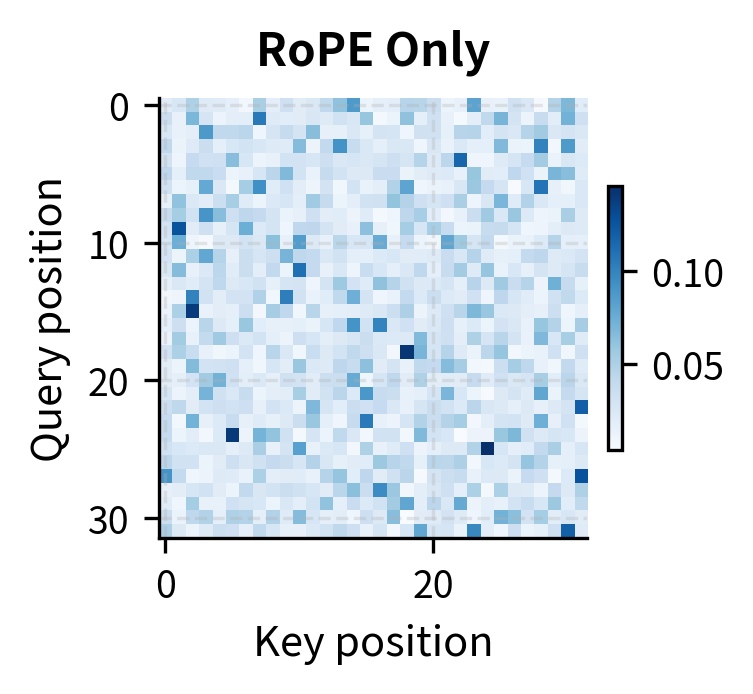

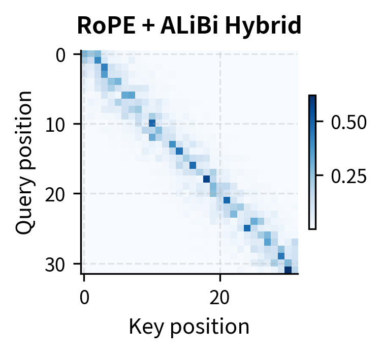
The hybrid pattern combines the best of both approaches. RoPE alone allows attention based on content matching regardless of distance (visible in the off-diagonal high-attention cells). ALiBi alone creates a strong recency bias that may miss relevant distant context. The hybrid maintains ALiBi's locality preference while allowing RoPE's content-based matching to override it when the content match is strong enough.
Current Best Practices
After examining all these methods and their trade-offs, what should you actually use? The answer depends on your specific requirements, but some patterns have emerged as industry best practices.
Decision Framework
The following framework helps navigate the choice:
1. What is your maximum context length requirement?
- Fixed, moderate length (≤4K): Any method works well
- Fixed, long length (4K-32K): Prefer RoPE or ALiBi
- Variable/unknown length: Prefer ALiBi (best extrapolation)
2. How important is extrapolation beyond training length?
- Not needed: Learned embeddings offer flexibility
- Moderate (2-4x): RoPE with interpolation
- Extreme (>4x): ALiBi
3. What are your computational constraints?
- Minimal overhead needed: Sinusoidal, Learned, or ALiBi
- Moderate overhead acceptable: RoPE
- Maximum flexibility needed: Relative position encoding
4. Is implementation simplicity a priority?
- Yes: Sinusoidal or Learned (modify only input)
- Somewhat: ALiBi (simple bias addition)
- Not critical: RoPE (best overall trade-off)
Current Industry Choices (as of 2024):
- LLaMA/Mistral/Most open models: RoPE
- BLOOM: ALiBi
- GPT-3: Learned embeddings
- Original Transformer: Sinusoidal
Summary Comparison Table
Let's create a comprehensive comparison across all dimensions we've discussed.
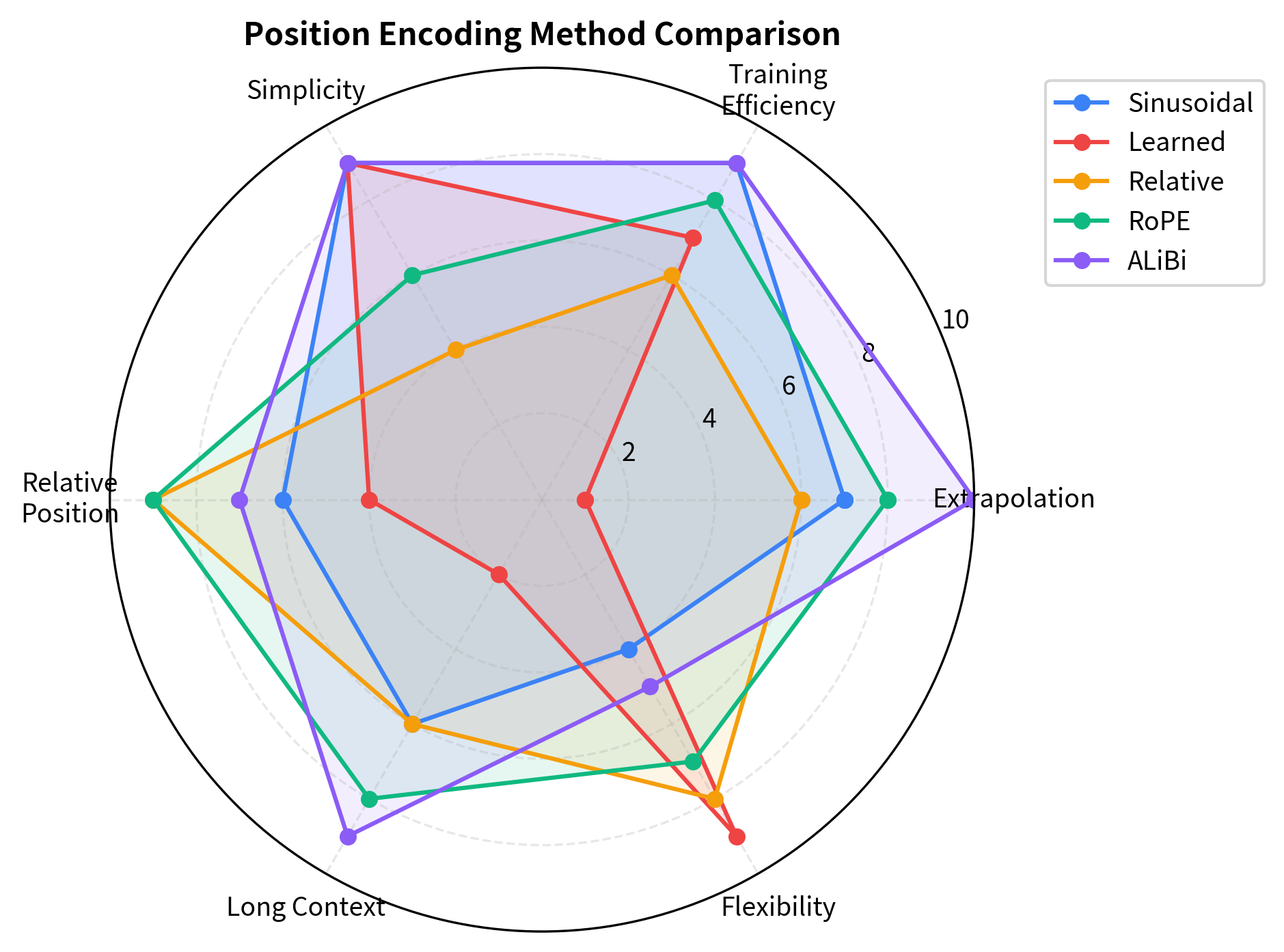
The radar chart reveals distinct profiles for each method. ALiBi dominates on extrapolation and simplicity, making it ideal for applications requiring length generalization with minimal engineering overhead. RoPE offers the best overall balance, which explains its adoption by most modern open-source language models. Learned embeddings sacrifice extrapolation for maximum flexibility, suitable when the context length is fixed and task-specific patterns are expected. Sinusoidal encoding provides a solid baseline with no parameters, still useful for some applications despite being the original approach.
Limitations and Practical Implications
Despite the progress in position encoding, fundamental challenges remain that no current method fully solves.
No method eliminates the need for long-context training. Even with perfect extrapolation of position representations, models struggle with long-range dependencies they haven't seen during training. The attention patterns learned on 2K contexts may not transfer to 100K contexts, regardless of how well the position encoding generalizes. This is why models like GPT-4 with 128K context are trained on long documents, not simply extrapolated from shorter training.
Computational costs still scale quadratically. Position encoding determines how positions are represented, not how they're processed. Standard attention still requires computing all pairwise interactions, which scales as with sequence length . This means doubling the context length quadruples the computation, regardless of which position encoding is used. Position encoding innovations must be combined with sparse attention, linear attention, or other efficiency techniques for truly long contexts.
Task-specific patterns may require task-specific encoding. Code has different positional structure than natural language. Mathematical proofs have different structure than dialogue. A single position encoding may not capture all relevant patterns. Some research explores task-adaptive or learned position encoding schemes, but no universally optimal approach exists.
Relative position has limits too. While relative position often matters more than absolute position for linguistic relationships, some tasks genuinely need absolute position. Document retrieval, citation matching, and structured data processing may benefit from knowing that a token is at position 7 of a table, not just that it's 3 positions from another token.
The field continues to evolve. Newer approaches like xPos, Contextual Position Encoding, and Continuous Position Embeddings address specific limitations, while the core trade-offs remain. Understanding these trade-offs, as we've explored throughout this chapter, enables informed decisions about which method best suits your application.
Summary
This chapter compared position encoding methods across the dimensions that matter for practical deployment. Each method embodies different design philosophies and makes different trade-offs.
Key takeaways:
-
Extrapolation capabilities vary dramatically. ALiBi was designed for extrapolation and handles it best. RoPE with interpolation techniques extends well. Sinusoidal extrapolates mathematically but may not preserve learned patterns. Learned embeddings fail completely beyond training length.
-
Implementation complexity differs by integration point. Methods that modify input embeddings (sinusoidal, learned) are simplest to implement. ALiBi adds bias to attention scores. RoPE transforms Q and K. Relative position encoding requires the most extensive modifications.
-
Parameter costs matter at scale. Learned embeddings add parameters proportional to context length times embedding dimension. Formula-based methods (sinusoidal, RoPE, ALiBi) add zero parameters. For long-context models, this difference becomes significant.
-
Training dynamics favor structured methods. Formula-based encodings provide useful inductive biases from the start, accelerating initial learning. Learned embeddings must discover structure from scratch but can eventually adapt to task-specific patterns.
-
Hybrid approaches combine strengths. RoPE + ALiBi combines content-based matching with explicit distance penalties. Block-wise encoding handles local and global context differently. No single pure method is optimal for all scenarios.
-
Current best practice converges on RoPE. Most modern open-source language models use RoPE, with interpolation techniques for context extension. ALiBi remains popular for models prioritizing length generalization. Learned embeddings persist in some architectures for their flexibility.
Position encoding remains an active research area, with new methods continually addressing the limitations of existing approaches. The framework developed in this chapter, evaluating methods across extrapolation, efficiency, complexity, and practical performance, provides a foundation for understanding future developments and making informed architecture decisions.
Key Parameters
When implementing position encoding methods, several parameters significantly influence behavior and performance. Understanding these helps you configure each method appropriately for your use case.
Common Parameters Across Methods
-
max_len/max_position_embeddings: Maximum sequence length the model can handle. For learned embeddings, this is a hard limit. For formula-based methods, it determines pre-computation range but doesn't restrict extrapolation. -
embed_dim/d_model: Dimension of position vectors. Must match the token embedding dimension for additive methods (sinusoidal, learned). For RoPE, determines the number of rotation frequency pairs.
Sinusoidal Encoding
base(default: 10000): Controls the wavelength range. Higher values create longer wavelengths, spreading position information across more positions. The original Transformer used 10000, which works well for sequences up to several thousand tokens.
Learned Embeddings
- Initialization scale: Random initialization magnitude affects training dynamics. Small values (0.01-0.02) prevent position information from dominating early training.
RoPE
-
base(default: 10000): Same role as sinusoidal, controlling frequency decay across dimensions. Lower values create faster-varying patterns, potentially better for short-range dependencies. -
scaling_factor: For position interpolation, determines how positions are compressed. A factor of 2.0 compresses 8K positions into the 0-4K range the model saw during training.
ALiBi
-
num_heads: Number of attention heads determines the slope distribution. More heads provide finer-grained distance sensitivity across different attention patterns. -
Slope computation: Slopes follow a geometric sequence from to , where is the number of heads. Lower slopes (closer to 0) create gentler distance penalties for some heads.
Context Extension Parameters
-
alpha(NTK interpolation): Scaling factor for the frequency base. Values around 1.5-2.0 typically work well for 2-4x context extension. -
scale(linear interpolation): Ratio of training length to target length. Computed astrain_len / target_len.
Quiz
Ready to test your understanding? Take this quick quiz to reinforce what you've learned about comparing position encoding methods in transformers.

Comments