RMSNorm: Efficient Normalization for Modern LLMs

Layer normalization stabilizes training by centering activations around zero and scaling them to unit variance. But does it need both operations? RMSNorm, introduced by Zhang and Sennrich in 2019, answers with a surprising finding: mean centering is often unnecessary. By removing it, RMSNorm achieves comparable or better performance with reduced computational cost.

This simplification might seem minor, but it matters in practice. Modern large language models perform normalization at every layer, often multiple times per transformer block. When you're running billions of forward passes during training or serving millions of inference requests, even small efficiency gains compound significantly. LLaMA, Mistral, and most contemporary open-source LLMs have adopted RMSNorm as their standard normalization layer.

To appreciate what RMSNorm removes and why that removal works, we first need to understand what LayerNorm does and the distinct roles of its two operations.

When a vector of activations passes through a neural network layer, its values can drift to arbitrary scales. Some elements might be large and positive, others small and negative. This variability creates problems: gradients become uneven, optimization landscapes shift during training, and networks become sensitive to initialization. LayerNorm addresses this by forcing activations into a consistent statistical profile.

Given an input vector $\mathbf{x}$ with $d$ elements, LayerNorm performs two sequential transformations:

1. Centering: Subtract the mean so values cluster around zero
2. Scaling: Divide by the standard deviation so values have unit spread

After these operations, it applies learnable parameters to let the network recover any distribution it needs. The complete formula is:

where:

• $\mathbf{x} \in \mathbb{R}^d$: the input vector to normalize
• $\mu = \frac{1}{d} \sum_{i=1}^{d} x_i$: the mean of the input elements
• $\sigma^2 = \frac{1}{d} \sum_{i=1}^{d} (x_i - \mu)^2$: the variance of the input elements
• $\gamma \in \mathbb{R}^d$: learnable scale parameters (initialized to 1)
• $\beta \in \mathbb{R}^d$: learnable shift parameters (initialized to 0)
• $\epsilon$: a small constant for numerical stability (typically $10^{-5}$ or $10^{-6}$)
• $\odot$: element-wise multiplication

The numerator $(\mathbf{x} - \mu)$ centers the data: every element is adjusted so the new mean is exactly zero. The denominator $\sqrt{\sigma^2 + \epsilon}$ scales the data: it measures how spread out the values are and shrinks or expands them to unit variance. Together, these operations produce a standardized distribution, and the learnable parameters $\gamma$ and $\beta$ then reshape it as the network sees fit.

But here's the key question Zhang and Sennrich asked: do we actually need both operations?

The intuition behind centering is compelling. Shifting activations to have zero mean creates a symmetric distribution around the origin. Optimization algorithms can work with positive and negative gradients more evenly. Activations don't accumulate bias through layers. It seems like a good idea.

But consider what happens after normalization. The learnable shift parameter $\beta$ can move the output to any mean value. If the network learns $\beta = \mu$ (setting the shift equal to the original mean), it completely undoes the centering we just performed. The network has the freedom to recover the original distribution.

This observation reveals something subtle: centering is not a hard constraint. It's a soft regularization that the network can override if needed. The real question becomes whether the network benefits enough from the centering operation to justify its computational cost.

The cost is not trivial. Computing the mean requires summing all $d$ elements and dividing. Then we subtract this mean from every element. Only after that can we compute the variance (which requires another pass through the data). If we could skip the centering step entirely, we'd eliminate:

• One reduction operation (computing $\mu$)
• $d$ subtraction operations (computing $x_i - \mu$ for each element)
• Dependency chains that limit parallelization

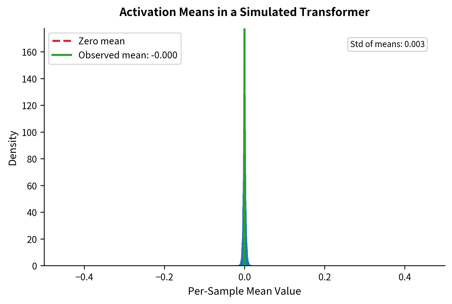
Zhang and Sennrich hypothesized that in transformer architectures with proper initialization, activations naturally stay roughly centered anyway. Residual connections add the original input back, preventing values from drifting too far from zero. If activations are already near-centered, explicitly centering them might be redundant.

RMSNorm tests this hypothesis by removing mean centering entirely. Instead of measuring spread around the mean (standard deviation), it measures spread around zero (root mean square). This single change eliminates the need to compute or subtract the mean.

The root mean square (RMS) of a vector captures its typical magnitude:

where:

• $\text{RMS}(\mathbf{x})$: the root mean square of the input vector
• $d$: the number of elements in the input vector
• $x_i$: the $i$-th element of the input vector
• $\frac{1}{d} \sum_{i=1}^{d} x_i^2$: the mean of squared values (the "mean square")

Think of RMS as answering the question: "How big are these values, on average?" It squares each element (making everything positive), averages them, and takes the square root (returning to the original scale). Large values contribute more; small values contribute less. The result is a single number representing the typical magnitude.

Dividing by the RMS normalizes the vector to have unit RMS. Values that were large become order-1; values that were small stay small but in proportion. This is the core of RMSNorm:

Expanding the RMS definition:

where:

• $\gamma \in \mathbb{R}^d$: learnable scale parameters (initialized to 1)
• $\epsilon$: a small constant for numerical stability

Notice what's absent compared to LayerNorm:

• No mean subtraction ($\mathbf{x} - \mu$): We normalize around zero, not around the data's center
• No $\beta$ shift parameter: Since we don't center, we don't need to un-center

RMSNorm is purely a scaling operation. Each input element is divided by the same scalar (the RMS), then multiplied by its corresponding learned scale factor. The operation preserves the relative relationships between elements while bringing everything to a consistent magnitude.

We've claimed that RMSNorm works because activations in neural networks tend to be near-centered. But how near is near enough? To answer this precisely, we need to understand the mathematical relationship between what RMSNorm computes (the RMS) and what LayerNorm computes (the standard deviation).

This section derives the exact connection between these two quantities. The derivation is worth following carefully because it reveals a beautiful geometric relationship and tells us exactly when the two normalizations diverge.

We want to express $\text{RMS}(\mathbf{x})$ in terms of $\sigma$ (the standard deviation) and $\mu$ (the mean). If we can do this, we'll know how much the two normalizations differ based on the mean alone.

Start with the definition of variance, which measures how spread out values are around their mean:

where:

• $\sigma^2$: the variance of the input vector
• $d$: the number of elements in the vector
• $x_i$: the $i$-th element of the input vector
• $\mu$: the mean of the input elements

This formula takes each element, measures its distance from the mean, squares that distance, and averages all the squared distances. The square root of variance gives us the standard deviation $\sigma$, which has the same units as the original data.

Our strategy is to expand the variance formula and recognize familiar terms. We'll use the algebraic identity $(a - b)^2 = a^2 - 2ab + b^2$ to expand the squared term:

Now we can distribute the sum across the three terms. Each term gets its own summation:

Let's simplify each term:

• First term: $\frac{1}{d} \sum_{i=1}^{d} x_i^2$ is the mean of squared values. This is exactly $\text{RMS}(\mathbf{x})^2$.
• Second term: The sum $\sum_{i=1}^{d} x_i$ equals $d \cdot \mu$ by the definition of mean. So this term becomes $\frac{2\mu}{d} \cdot (d\mu) = 2\mu^2$.
• Third term: We're summing the constant $\mu^2$ exactly $d$ times, so this equals $\frac{d \cdot \mu^2}{d} = \mu^2$.

Substituting these simplifications:

Rearranging to isolate the RMS:

Taking square roots of both sides:

where:

• $\text{RMS}(\mathbf{x})$: the root mean square of the input vector
• $\sigma$: the standard deviation of the input vector
• $\mu$: the mean of the input vector

This formula has a beautiful geometric meaning. Think of $\sigma$ and $\mu$ as the two legs of a right triangle. The RMS is the hypotenuse. The Pythagorean theorem tells us that $\text{hypotenuse}^2 = \text{leg}_1^2 + \text{leg}_2^2$, which is exactly what we derived.

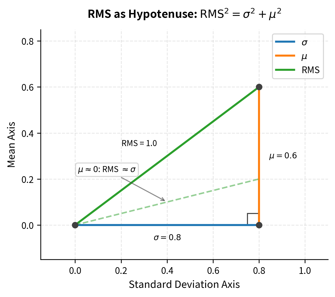
This geometric picture immediately reveals when RMSNorm and LayerNorm behave similarly:

• When $\mu = 0$: The triangle collapses to a line. The hypotenuse equals the remaining leg: $\text{RMS} = \sigma$. The two normalizations are identical.
• When $\mu$ is small relative to $\sigma$: The triangle is nearly flat. The hypotenuse is only slightly longer than $\sigma$. The normalizations are nearly equivalent.
• When $\mu$ is comparable to or larger than $\sigma$: The triangle is more equilateral or tall. The hypotenuse differs significantly from $\sigma$. The normalizations diverge.

The crucial question for practical use becomes: in real neural networks, how large is $\mu$ compared to $\sigma$?

The outputs are highly correlated but not identical. The differences arise from the mean subtraction in LayerNorm. Let's visualize how the two normalizations compare across different input distributions.

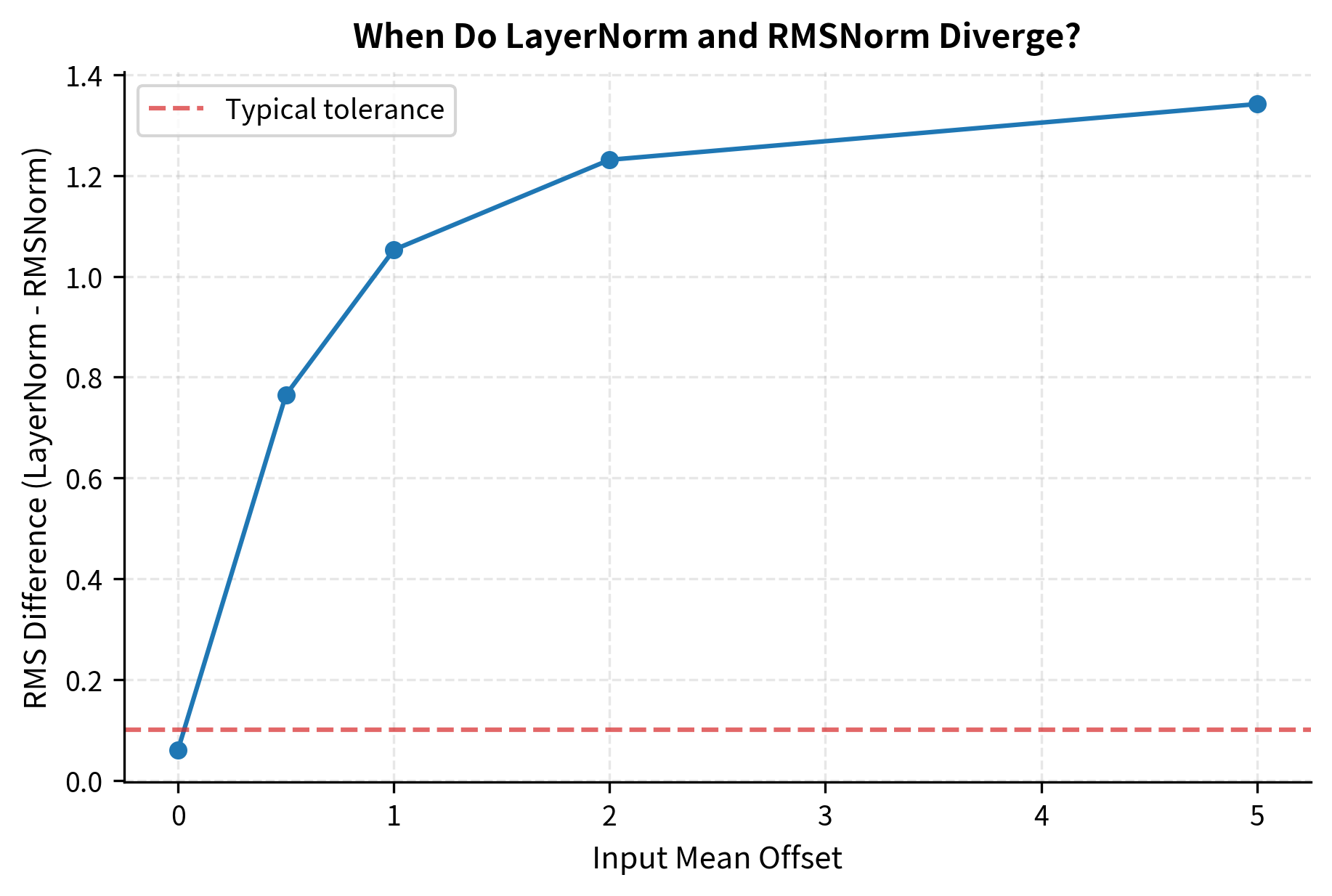
The key insight emerges: when inputs are approximately centered (mean near zero), the two normalizations are nearly equivalent. In deep neural networks with proper initialization and residual connections, activations tend to stay roughly centered. This explains why RMSNorm works as well as LayerNorm in practice.

With the mathematical foundation established, let's translate our understanding into working code. We'll build RMSNorm from first principles, compare it with LayerNorm, and observe how the two behave on real data.

The implementation follows directly from the formula. For each input vector, we need to:

1. Square all elements
2. Compute the mean of these squares
3. Take the square root (adding epsilon for stability)
4. Divide the original input by this RMS value
5. Multiply by the learnable scale parameters

Let's implement both RMSNorm and LayerNorm as Python classes:

With both classes defined, let's apply them to realistic input data and examine the output statistics. We'll use a tensor shaped like typical transformer activations: batch size 16, sequence length 128, hidden dimension 512.

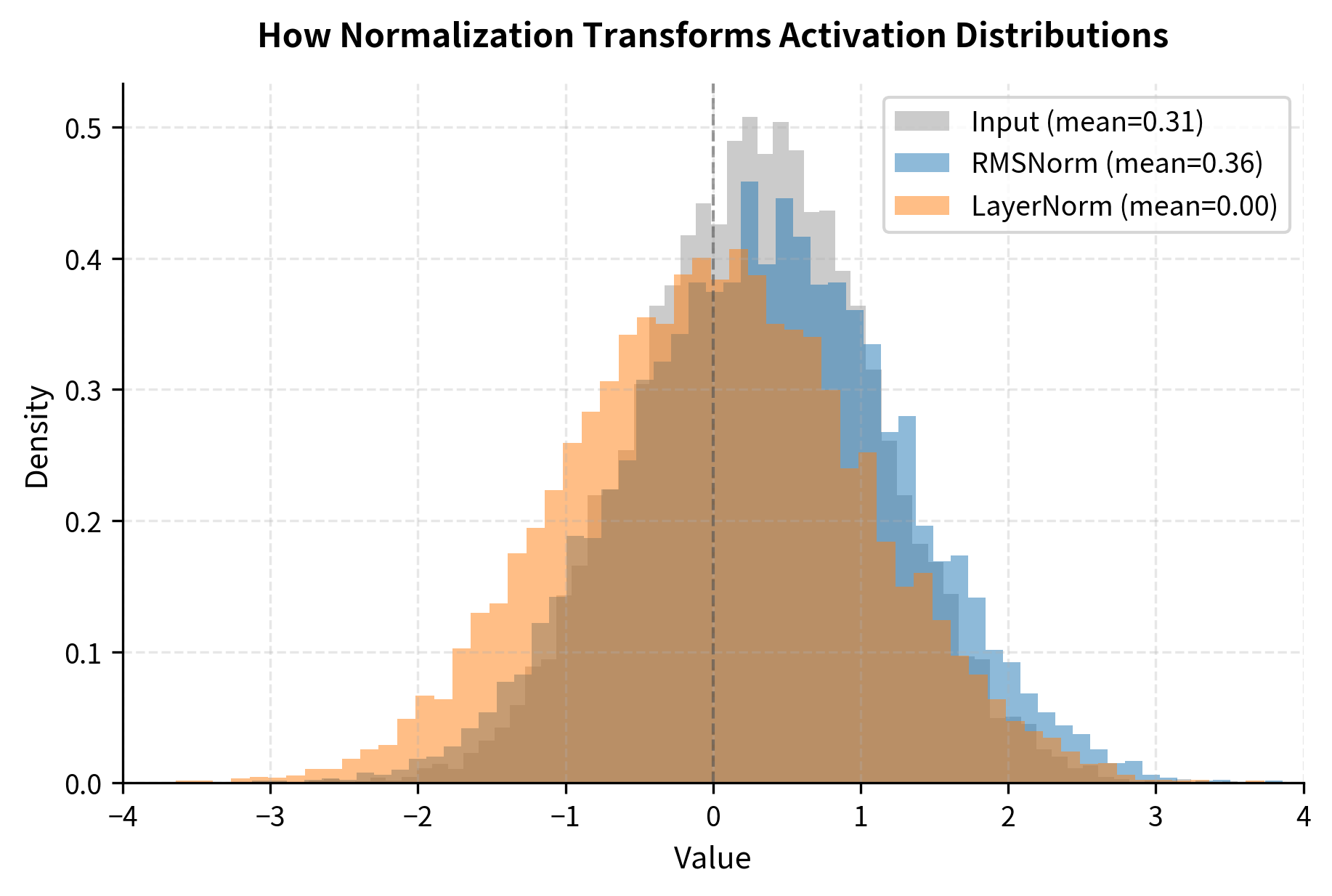
The statistics reveal the key behavioral difference between the two normalizations. Look at the RMS values: RMSNorm produces output with RMS close to 1.0, which is exactly what it's designed to do. The mean, however, is not forced to zero.

LayerNorm tells a different story. Its output has near-zero mean (by design) and unit standard deviation. Because the mean is zero, the RMS and standard deviation are approximately equal, confirming our earlier mathematical derivation.

Despite these differences, both approaches accomplish the primary goal: they normalize the magnitude of activations to a consistent scale, which is what matters for stable training.

The primary motivation for RMSNorm is computational efficiency. Let's count the operations required for each normalization.

LayerNorm operations per element:

1. Compute mean: 1 addition (accumulated) + 1 division (shared across elements)
2. Subtract mean: 1 subtraction
3. Compute squared difference: 1 subtraction + 1 multiplication
4. Compute variance: 1 addition (accumulated) + 1 division (shared)
5. Add epsilon and take square root: 1 addition + 1 sqrt (shared)
6. Divide by std: 1 division
7. Scale by gamma and add beta: 1 multiplication + 1 addition

RMSNorm operations per element:

1. Square each element: 1 multiplication
2. Compute mean of squares: 1 addition (accumulated) + 1 division (shared)
3. Add epsilon and take square root: 1 addition + 1 sqrt (shared)
4. Divide by RMS: 1 division
5. Scale by gamma: 1 multiplication

The reduction in operations comes from eliminating the mean computation and subtraction, plus removing the bias parameter. Let's measure the actual speedup:

The benchmark shows RMSNorm consistently outperforming LayerNorm across all dimensions. The speedup factor varies slightly with dimension, but RMSNorm is typically 10-30% faster in this CPU-based NumPy implementation. On GPUs with optimized CUDA kernels, the speedup is typically in the 5-15% range due to different bottlenecks.

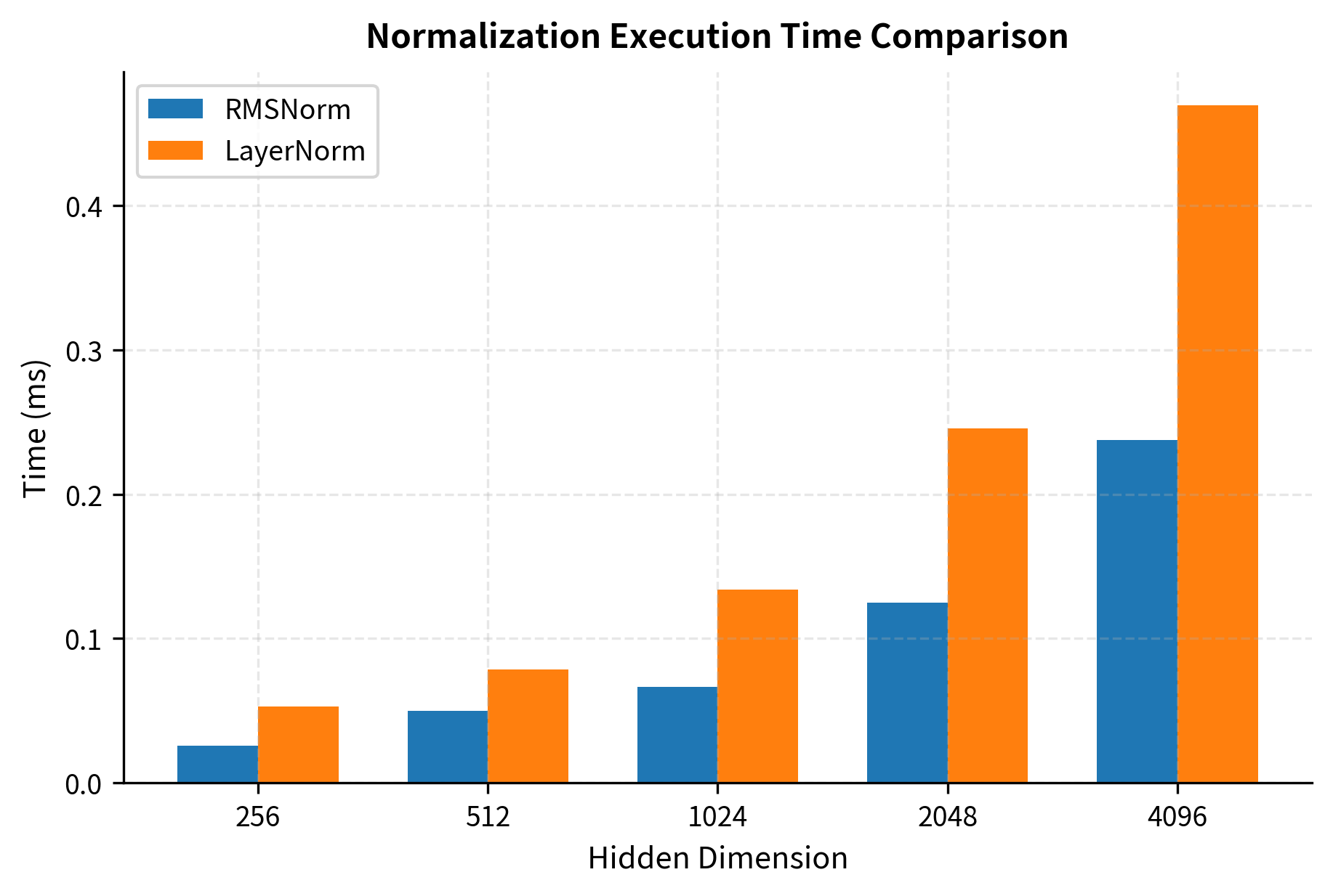
The speedup varies depending on hardware and implementation details. On GPUs with optimized kernels, the speedup is typically 5-15% for RMSNorm. While this might seem modest, it adds up significantly in large models where normalization is applied at every layer.

Beyond computational cost, RMSNorm also reduces the number of parameters. LayerNorm has two learnable vectors per layer ($\gamma$ and $\beta$), while RMSNorm has only one ($\gamma$).

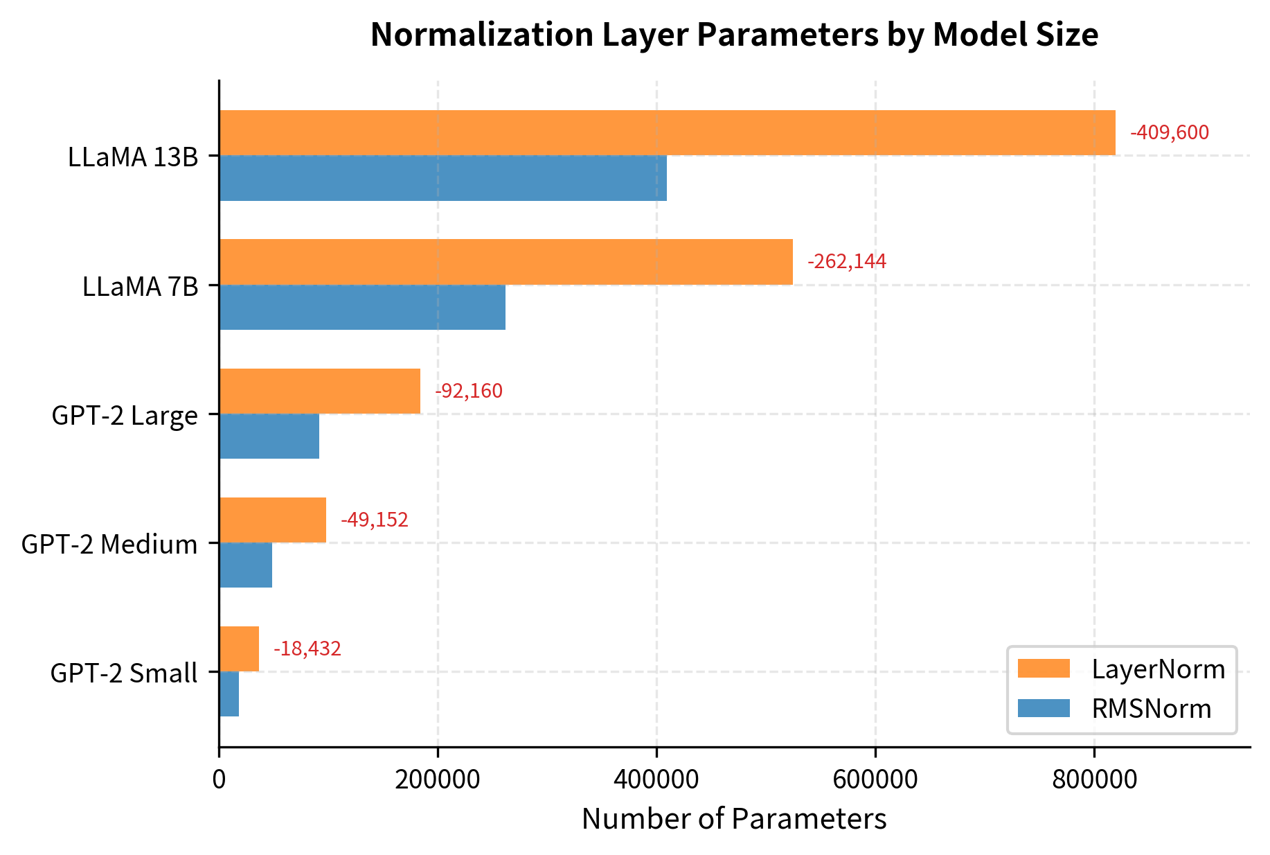
The parameter savings scale with model size. For LLaMA 7B, switching from LayerNorm to RMSNorm saves over 500,000 parameters. While this is less than 0.01% of the total model size, these parameters also consume memory bandwidth during inference and require gradient computation during training. Every reduction helps.

Understanding the backward pass helps us see why RMSNorm is computationally cheaper. The gradient computation for RMSNorm is simpler because it doesn't need to backpropagate through the mean computation.

Consider the forward pass where each output element $y_i$ is computed as:

where:

• $y_i$: the $i$-th element of the output
• $\gamma_i$: the $i$-th learnable scale parameter
• $x_i$: the $i$-th element of the input
• $\text{RMS}(\mathbf{x})$: the root mean square computed over all input elements

To compute gradients, we need to determine how each input element $x_j$ affects each output element $y_i$. This requires the partial derivative:

For notational convenience, let $r = \text{RMS}(\mathbf{x}) = \sqrt{\frac{1}{d}\sum_k x_k^2}$. We first need the derivative of $r$ with respect to $x_j$. Using the chain rule on the square root and sum:

where:

• $\frac{\partial r}{\partial x_j}$: how much the RMS changes when $x_j$ changes
• $x_j$: the $j$-th input element (the one we're differentiating with respect to)
• $d$: the dimension of the input vector
• $r$: the RMS value (appears in the denominator because of the square root derivative)

Now we apply the quotient rule to $\frac{x_i}{r}$. The quotient rule states that $\frac{d}{dx}\left(\frac{u}{v}\right) = \frac{u'v - uv'}{v^2}$:

where:

• $\delta_{ij}$: the Kronecker delta, equal to 1 if $i = j$ and 0 otherwise
• The first term $\frac{\delta_{ij}}{r}$: the direct effect when $i = j$ (changing $x_j$ directly changes the numerator $x_i$)
• The second term $\frac{x_i x_j}{d \cdot r^3}$: the indirect effect through the RMS in the denominator (changing any $x_j$ affects the RMS, which affects all outputs)

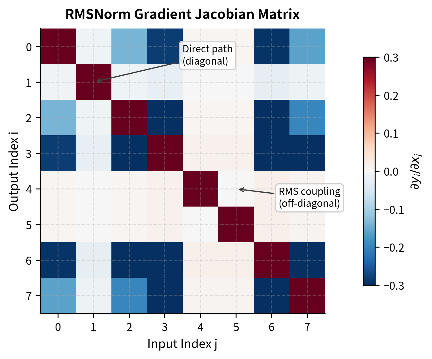
To compute the gradient of a loss $L$ with respect to input $x_j$, we apply the chain rule, summing over all output elements:

The Kronecker delta $\delta_{ij}$ selects only the $i = j$ term from the sum for the first part, giving us:

where:

• $\frac{\partial L}{\partial y_j}$: the upstream gradient for output element $j$
• The first term: the direct gradient path from $x_j$ through $y_j$
• The second term: the indirect gradient path where $x_j$ affects all outputs via the shared RMS denominator
• The sum $\sum_i \gamma_i \cdot x_i \cdot \frac{\partial L}{\partial y_i}$: aggregates the indirect effects across all output dimensions

The gradient check confirms our analytical backward pass implementation is correct. A relative error below $10^{-4}$ indicates that the analytical and numerical gradients agree to high precision, validating both the mathematical derivation and the code implementation.

The theoretical efficiency of RMSNorm is clear, but does it maintain model quality? Let's compare the two normalizations on a simple task to see their behavior during training.

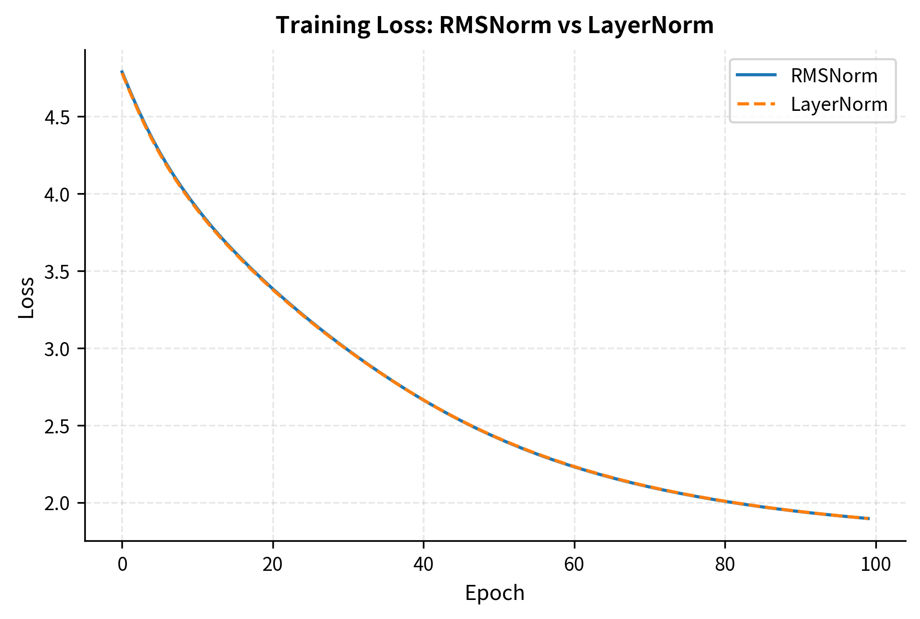
Both normalizations converge to similar loss values, confirming that RMSNorm doesn't sacrifice model quality for efficiency. In larger-scale experiments on language modeling benchmarks, RMSNorm has been shown to match or slightly exceed LayerNorm performance.

RMSNorm has become the normalization of choice for most modern large language models. Let's examine how it's typically used in practice.

The LLaMA family of models uses RMSNorm with a specific configuration:

The key insight is computing normalization in float32 even when the model uses float16 or bfloat16 for other operations. This prevents numerical instability from small RMS values in reduced precision.

Modern transformers use RMSNorm in a pre-normalization configuration, applying it before each sub-layer rather than after:

The pre-norm placement ensures that inputs to each sub-layer are normalized, stabilizing gradients throughout the network. This has become standard practice after research showed it improves training stability, especially for very deep models.

RMSNorm's simplicity comes with trade-offs that are worth understanding.

When mean centering matters. If the input distribution has a significant non-zero mean, RMSNorm and LayerNorm produce different outputs. In most transformer architectures with proper initialization and residual connections, activations remain approximately centered, making this difference negligible. However, if you're applying RMSNorm to data with known biases (like all-positive image features), the lack of centering could affect downstream layers.

Interaction with other components. RMSNorm's lack of a $\beta$ bias parameter means it can't shift the output distribution. In pre-norm architectures, this is fine because the subsequent linear layers can learn any necessary bias. But in post-norm configurations or when RMSNorm is the final layer before output, you might need an explicit bias term elsewhere.

Numerical precision. RMSNorm divides by a single scalar (the RMS), while LayerNorm divides by the standard deviation after subtracting the mean. In rare cases with extreme values, RMSNorm can be less stable because the RMS includes the squared mean contribution. Modern implementations address this by computing in float32 even for mixed-precision training.

Not a drop-in replacement. While RMSNorm can replace LayerNorm in most architectures, models pre-trained with LayerNorm should not have their normalization layers swapped without retraining. The learned $\gamma$ parameters adapt to the specific normalization behavior.

For production use, here's a robust implementation that handles edge cases:

The output RMS is close to 1.0, confirming the normalization is working correctly. The shape is preserved, and the layer's extra_repr shows the configured dimension and epsilon value.

The torch.rsqrt function computes $1/\sqrt{x}$ in a single operation, which is faster than separate division and square root. The type_as call ensures the output matches the input dtype for mixed precision training.

When implementing or using RMSNorm, several parameters control its behavior:

• dim: The feature dimension to normalize over. This should match the hidden dimension of your model. For transformer models, this is typically the embedding dimension (e.g., 768 for BERT-base, 4096 for LLaMA-7B).

• eps (default: $10^{-6}$ to $10^{-5}$): A small constant added to the RMS before division for numerical stability. Prevents division by zero when all input values are near zero. LLaMA uses $10^{-5}$, while some implementations use $10^{-6}$. Smaller values provide more precision but risk numerical instability in low-precision training.

• weight ($\gamma$): The learnable scale parameter, a vector of dimension dim. Initialized to ones, allowing the network to learn per-feature scaling. Unlike LayerNorm, RMSNorm has no bias ($\beta$) parameter.

• Computation dtype: For mixed-precision training (float16 or bfloat16), compute the normalization in float32 before casting back to the original dtype. This prevents numerical issues from small RMS values in reduced precision.

• Placement: Modern architectures use pre-normalization, applying RMSNorm before each attention and feed-forward sub-layer rather than after. This improves gradient flow and training stability.

RMSNorm simplifies layer normalization by removing mean centering, keeping only the scaling operation based on the root mean square of the input. This reduction provides computational savings and parameter efficiency while maintaining model quality.

Key takeaways from this chapter:

• RMS vs standard deviation: When inputs are centered around zero, RMS approximately equals the standard deviation. The relationship $\text{RMS}^2 = \sigma^2 + \mu^2$ shows they're equivalent when $\mu = 0$.

• Computational efficiency: RMSNorm eliminates the mean computation and subtraction, plus removes the $\beta$ bias parameter. This typically provides 5-15% speedup on GPUs.

• Parameter efficiency: With only $\gamma$ instead of both $\gamma$ and $\beta$, RMSNorm halves the normalization parameters per layer.

• Modern adoption: LLaMA, Mistral, and most contemporary LLMs use RMSNorm as their standard normalization layer, demonstrating its effectiveness at scale.

• Implementation details: Production implementations compute normalization in float32 for numerical stability and use rsqrt for efficiency.

• Pre-norm placement: RMSNorm is typically used in pre-normalization position, applied before each attention and feed-forward sub-layer.

The success of RMSNorm illustrates a broader principle in deep learning: simpler can be better. By questioning whether mean centering was truly necessary, researchers discovered that models could learn to work without it, gaining efficiency in the process.

Ready to test your understanding? Take this quick quiz to reinforce what you've learned about RMSNorm and its relationship to LayerNorm.