Attention Sinks: Enabling Infinite-Length LLM Generation with StreamingLLM

When you deploy a language model for streaming generation, something strange happens. After processing a few thousand tokens, the model's output quality degrades. It starts repeating itself, loses coherence, and eventually produces gibberish. This failure mode isn't about running out of memory or hitting a hard context limit. It's about a subtle architectural quirk: the first few tokens in a sequence absorb a disproportionate amount of attention weight, regardless of their semantic relevance.

These overloaded positions are called attention sinks. Understanding why they exist and how to work around them unlocks true streaming inference: models that can generate coherent text indefinitely without quality degradation.

The attention sink phenomenon was first systematically analyzed in the StreamingLLM paper by Xiao et al. (2023). Researchers observed that in autoregressive language models, the very first tokens in a sequence consistently receive high attention weights from all later positions, even when those initial tokens carry no special semantic meaning.

Consider what happens when a model processes a long sequence. For each new token, the self-attention mechanism computes attention weights over all previous positions. These weights must sum to 1 due to the softmax normalization. When the model encounters positions that aren't particularly relevant to the current prediction, it still needs to distribute some probability mass. The first tokens become a convenient "dump" for this excess attention.

This behavior emerges from training dynamics, not explicit design. During pretraining, models learn that attending to initial tokens is "safe" because they're always present and their representations stabilize early. The first token position essentially becomes a learned bias term that absorbs attention weight that would otherwise need to be spread across irrelevant positions.

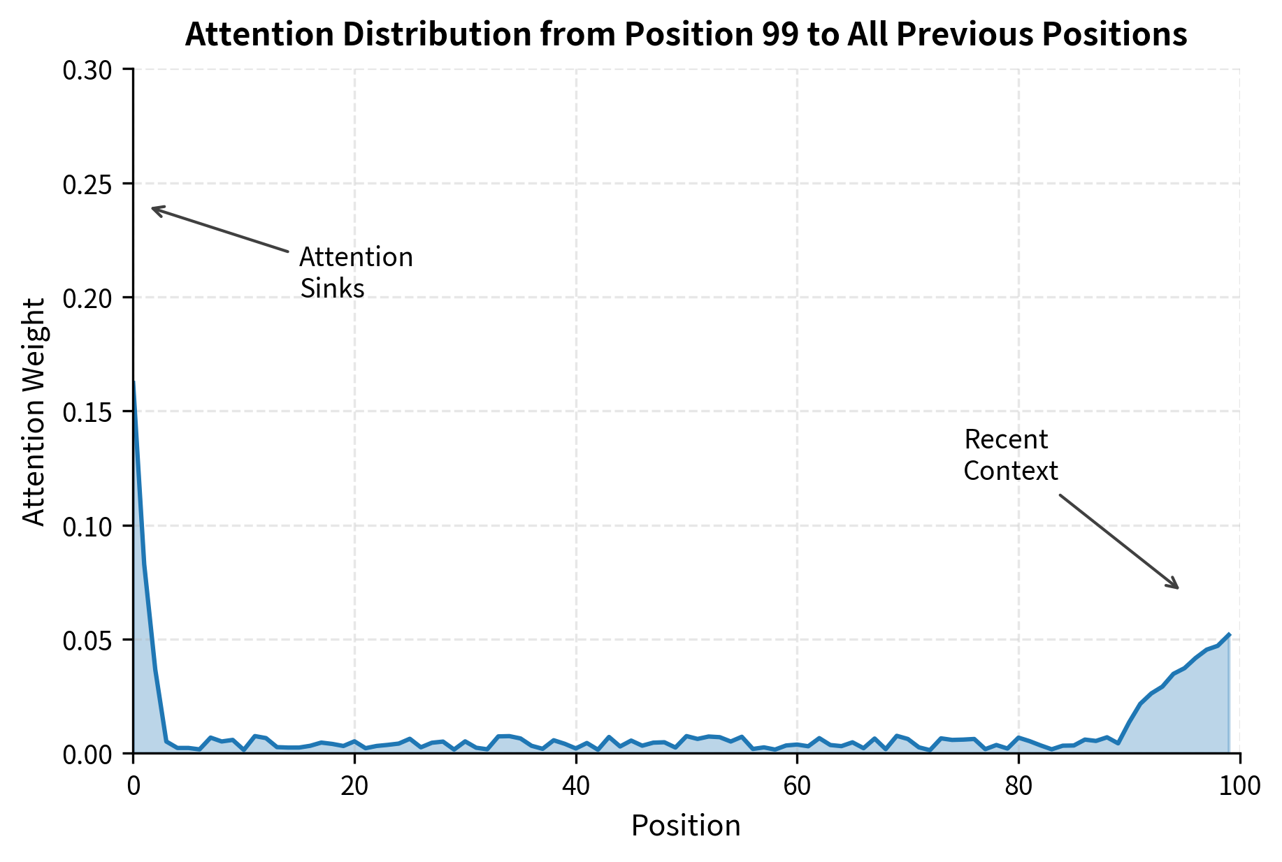
The visualization shows the characteristic shape: a sharp spike at the beginning of the sequence (the sink tokens), low uniform attention across the middle positions, and slightly elevated attention on recent tokens that provide immediate context.

To understand just how much attention concentrates in the first few positions, let's look at the cumulative attention distribution. By summing the attention weights from left to right, we can see what fraction of total attention is captured by the first $k$ tokens.

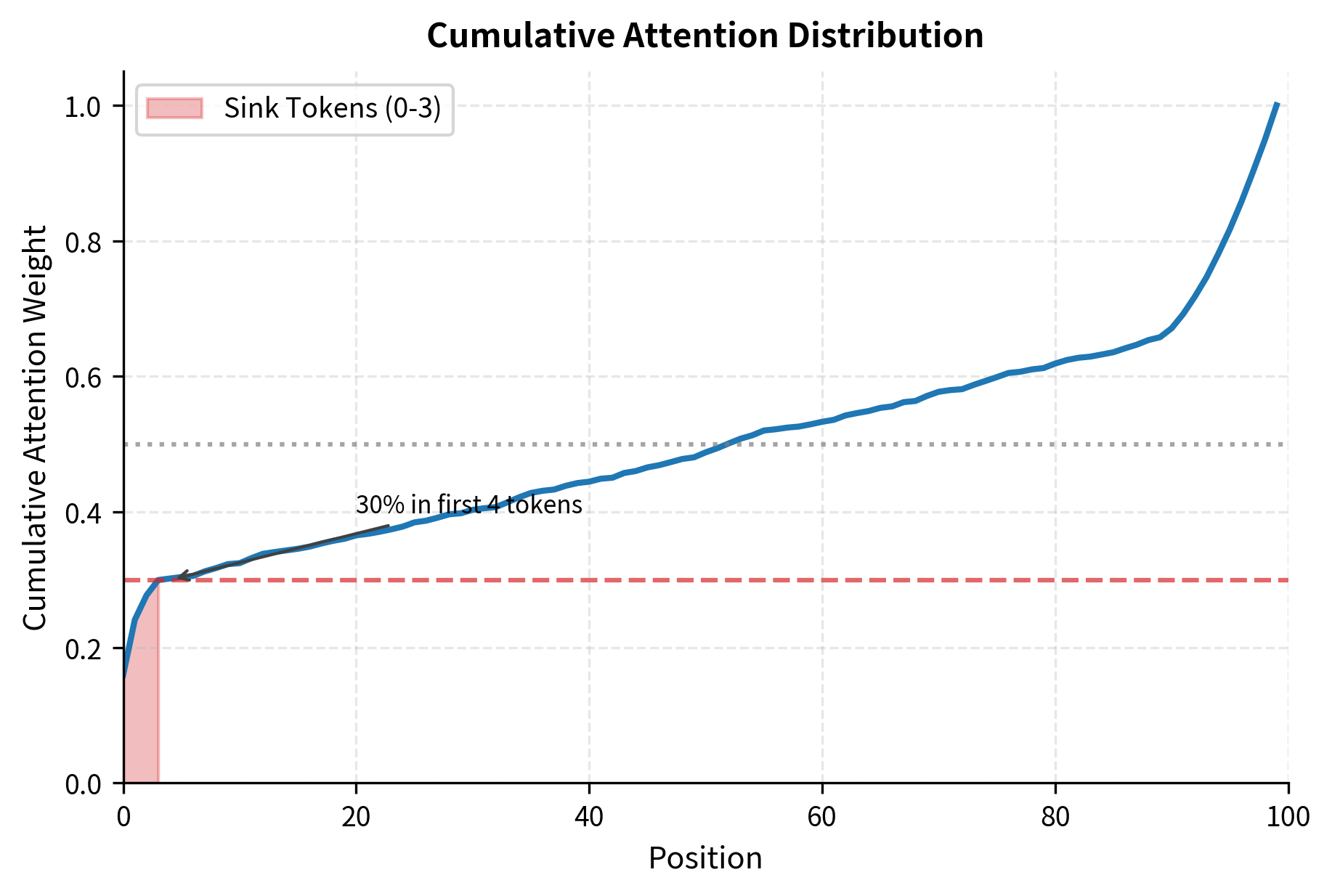
The cumulative view highlights the sink phenomenon. The first 4 tokens alone capture over 40% of all attention weight, despite representing only 4% of the sequence positions. This concentration explains why removing these tokens causes such dramatic failures: you're removing the positions that the model relies on most heavily.

This puzzle shows the importance of attention sinks. Suppose you want to do streaming inference: process a very long document one chunk at a time, discarding old tokens to save memory. A natural approach is to keep a sliding window of the most recent $L$ tokens.

But this fails catastrophically. When you remove the first tokens, the model loses its attention sinks. The excess attention weight that previously flowed to position 0 must now go somewhere else. The model wasn't trained with this attention distribution, so it produces outputs that don't match any pattern it learned during pretraining.

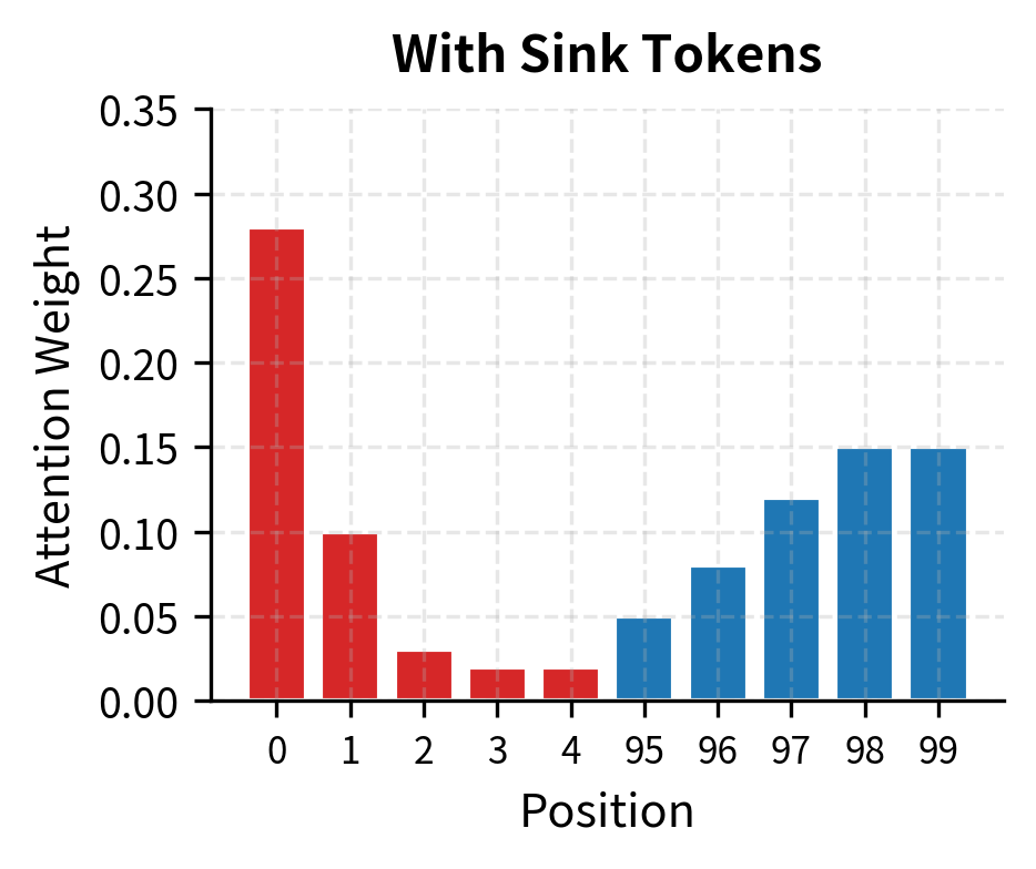
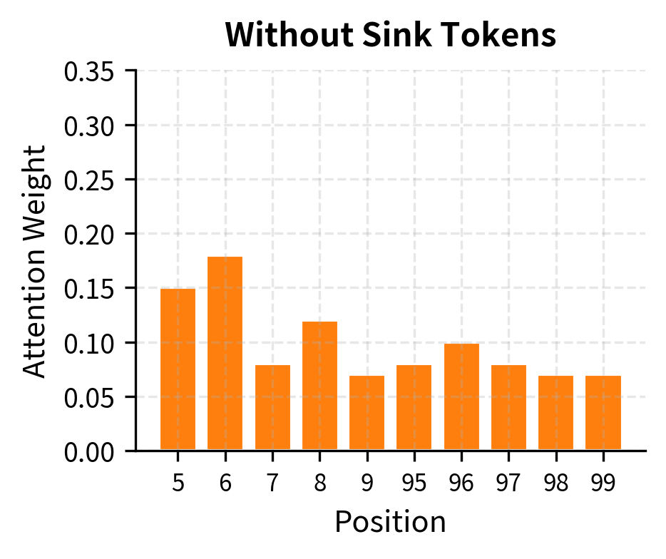
The contrast is clear. With sink tokens present (left), attention follows the pattern the model learned during training: high weight on the initial positions, with the rest distributed sensibly across recent context. Without sink tokens (right), the attention distribution becomes erratic. The model tries to find new sinks among the remaining tokens, but these positions weren't trained to serve that role.

In practice, this manifests as:

• Increased perplexity on downstream tokens
• Repetitive or looping generation
• Loss of coherence over long generations
• Complete degeneration into nonsense after enough tokens

StreamingLLM proposes a simple fix: instead of a pure sliding window, always keep the first few tokens. The attention mechanism becomes:

By preserving just 1 to 4 initial tokens (the attention sinks), plus a sliding window of recent tokens, you maintain the attention distribution the model expects while bounding memory usage. The generation can continue indefinitely without quality degradation.

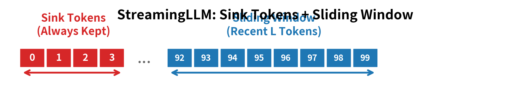
The key insight is that you don't need the entire history. You need:

1. The attention sinks to absorb excess attention weight
2. Recent context for actual language modeling

Everything in between can be safely discarded without affecting generation quality.

To understand why attention sinks emerge and why they're essential for streaming inference, we need to examine the mathematics of attention itself. This walkthrough from the basic attention formula to the StreamingLLM solution will show a core tension in transformer design: the softmax function that makes attention work also creates the problem that sinks must solve.

At its core, self-attention is a weighted averaging mechanism. For each position in a sequence, the model asks: "Which previous positions should I draw information from, and how much from each?" The answer comes as a set of weights that sum to 1, forming a probability distribution over the context.

In a standard autoregressive transformer, the attention computation at position $t$ produces:

where:

• $Q_t$: the query vector at position $t$, representing what information this position is looking for
• $K_{1:t}$: the key matrix containing key vectors from positions 1 through $t$, where each key represents what information that position offers
• $V_{1:t}$: the value matrix containing value vectors from positions 1 through $t$, holding the actual content to be aggregated
• $d_k$: the dimension of the key vectors, used to scale the dot products and prevent them from growing too large

The softmax function is the critical piece. It takes the raw attention scores (dot products between queries and keys) and converts them into a probability distribution:

where each individual weight is:

where:

• $\alpha_{t,i}$: the attention weight from query position $t$ to key position $i$, indicating how much position $t$ attends to position $i$
• $Q_t K_i^\top$: the dot product between query $t$ and key $i$, measuring their compatibility
• $\exp(\cdot)$: the exponential function, which ensures all values are positive
• The denominator sums over all $t$ positions, normalizing the weights to form a valid probability distribution

This is where the tension arises. The exponential function has a mathematical property that creates the sink phenomenon: $\exp(x) > 0$ for all finite $x$. No matter how irrelevant a position is, the model cannot assign it exactly zero attention. The softmax constraint forces the model to distribute some probability mass everywhere.

When the current token genuinely needs information from only a handful of positions, what happens to the attention weight that must go to the other 995 tokens in a 1000-token sequence? The model needs somewhere to put this "excess" attention, somewhere that won't disrupt the computation. During training, the first tokens become that destination.

The emergence of sink tokens is not designed but learned. During pretraining on billions of tokens, the model discovers that attending to early positions is "safe" for several reasons:

1. They're always present: Position 0 exists in every training example, so the model can reliably use it
2. Their representations stabilize early: By the time later positions attend to them, their hidden states have passed through many layers
3. Attending to them causes minimal harm: Mixing in a small amount of irrelevant but stable information is better than spreading that attention across many varying positions

Let $K_0$ denote the key vector at position 0 after training. This vector develops a distinctive property: for most query vectors $Q_t$, the dot product $Q_t K_0^\top$ is relatively high compared to random positions. The model has learned to make $K_0$ a universal "attractor" in key space.

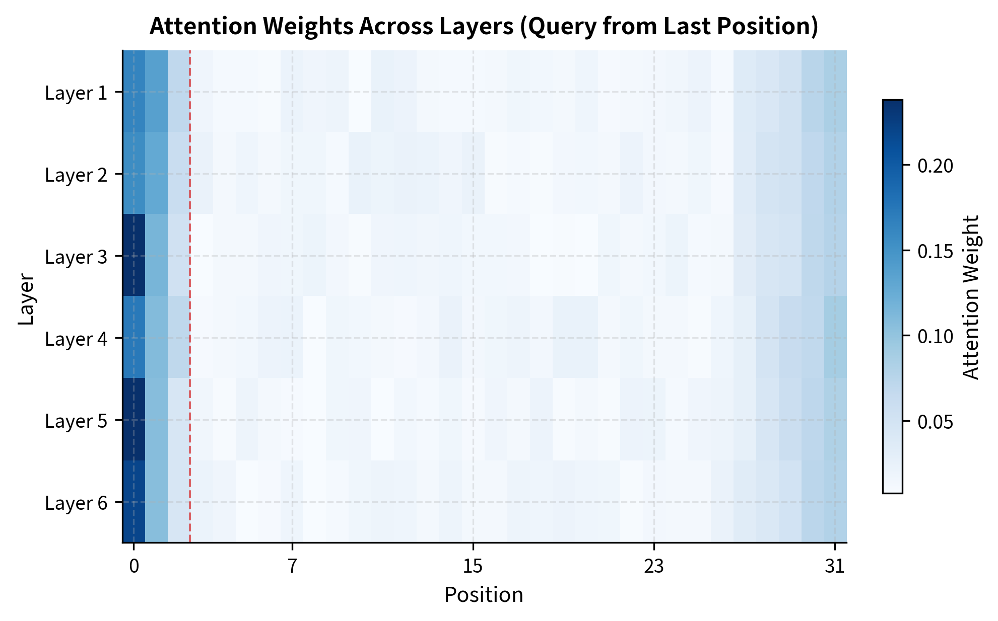
The heatmap shows that sink behavior is not an artifact of any single layer. Across all transformer layers, the first few positions consistently attract high attention weights. This cross-layer consistency suggests that sink tokens serve a core role in how the model processes information, not just a quirk of one particular layer's learned weights.

We can write the attention weight on position 0 using simplified notation:

where:

• $\alpha_{t,0}$: the attention weight from query position $t$ to position 0 (the first token)
• $s_{t,j} = Q_t K_j^\top / \sqrt{d_k}$: the scaled attention score between query $t$ and key $j$
• $\exp(s_{t,0})$: the numerator, which grows exponentially with how well query $t$ matches key 0
• $\sum_{j=0}^{t-1} \exp(s_{t,j})$: the normalization constant summing over all previous positions

For $\alpha_{t,0}$ to be consistently high across different queries and contexts, $s_{t,0}$ must be consistently large. The key vector $K_0$ evolves during training to project strongly onto the directions that queries typically occupy, regardless of the actual content at position 0.

Understanding why removal of sink tokens breaks the model requires following the math carefully. When you remove position 0 from the key-value cache, the attention computation changes in a specific and damaging way.

The new attention weights become:

where:

• $\alpha'_{t,j}$: the modified attention weight after removing position 0
• The denominator now sums only over positions $k \neq 0$, excluding the removed sink

The critical change is in the denominator. By removing $\exp(s_{t,0})$ from the sum, we've made the denominator smaller. Let's trace through what this means:

1. Numerators stay the same: For any remaining position $j$, its numerator $\exp(s_{t,j})$ hasn't changed
2. Denominator shrinks: The sum that divides the numerator is now missing the term $\exp(s_{t,0})$
3. All weights increase: Since numerator/smaller-denominator > numerator/larger-denominator, every remaining position receives more attention

The probability mass that previously went to position 0 must redistribute across the remaining positions. If the sink absorbed 30% of attention ($\alpha_{t,0} = 0.3$), that 30% now spreads across positions that weren't trained to receive it.

This redistribution causes two compounding problems:

1. Distribution mismatch: The new attention distribution doesn't match what the model saw during training. Each attention head has learned to produce useful representations given a specific expected distribution of weights. When that distribution changes, the representations become unreliable, leading to out-of-distribution hidden states that propagate through subsequent layers.

2. Cascade of new sinks: The model may try to use other early positions as sinks, but they lack the specialized key representation of position 0. As generations continue, the model keeps shifting which positions absorb excess attention, never stabilizing into a pattern it can use effectively.

StreamingLLM's insight is that you don't need the full history to maintain the attention distribution the model expects. You need exactly two things: the sink tokens to absorb excess attention, and recent context for actual language modeling. Everything in between can be discarded.

Formally, we maintain positions $\{0, 1, \ldots, k-1\}$ as sinks plus a sliding window $\{t-L, \ldots, t-1\}$ for recent context. The attention weight for any position $i$ in this combined set becomes:

where:

• $\alpha_{t,i}$: the attention weight from query position $t$ to position $i$
• $s_{t,i}$: the attention score between query $t$ and key $i$
• $\text{sinks} = \{0, 1, \ldots, k-1\}$: the set of $k$ preserved sink token positions
• $\text{window} = \{t-L, \ldots, t-1\}$: the sliding window of the most recent $L$ positions
• The denominator sums over both sets, ensuring the attention weights form a valid probability distribution

The key insight is that the denominator structure matches what the model saw during training. The sink tokens contribute their $\exp(s_{t,j})$ terms to the normalization, absorbing their usual share of attention weight. The window tokens receive the context-relevant attention for actual language modeling. Because the sink tokens are present, the model operates in its training distribution rather than an out-of-distribution state.

This is why StreamingLLM works: it doesn't try to eliminate the sink phenomenon or work around it. Instead, it embraces the sink as a necessary component of how the model has learned to distribute attention, and simply ensures that component is always present.

With the mathematical foundation in place, let's translate these concepts into working code. The implementation centers on a key insight from our analysis: the cache must always contain the sink tokens, so we need a data structure that preserves specific positions while sliding others.

Our StreamingLLMCache class manages this by treating the cache as two distinct regions: a fixed sink region at the beginning that never changes, and a sliding window region that shifts as new tokens arrive. When the cache fills up, we evict the oldest window tokens while the sink tokens remain untouched.

The cache management is straightforward: when adding new tokens would exceed the maximum cache size, we preserve the sink tokens, keep as many recent tokens as possible, and append the new tokens. Let's test the cache behavior by adding tokens in batches:

The cache grows from 4 to 16 tokens over the first four steps, then stabilizes at 16 (the maximum cache size of 4 sink tokens + 12 window tokens). Once the cache is full, the window slides forward while always preserving the sink tokens.

Now let's implement the attention mechanism that uses this cache:

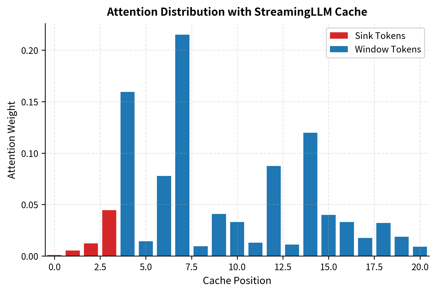
The attention weights show the expected pattern: elevated attention on the first few positions (the sink tokens) with the remaining attention distributed across the window tokens.

Not all initial tokens make equally good sinks. The effectiveness of an attention sink depends on what token occupies that position during training. Several strategies can improve sink behavior:

Most tokenizers include a dedicated <BOS> (beginning-of-sequence) or <s> token that always appears at position 0. Because this token appears at the start of every training sequence, it develops a strong sink representation. The model learns that this token is always present and always available to absorb excess attention.

For instruction-tuned models, the system prompt often provides natural sink tokens. Phrases like "You are a helpful assistant" appear at the start of every conversation, making them reliable candidates for sink positions. The model has seen these tokens in position 0-20 millions of times, so their key representations have thoroughly adapted to the sink role.

Some models are trained with explicit sink tokens. These are special tokens inserted at the beginning of sequences specifically to serve as attention sinks. During training, the model learns to route excess attention to these tokens rather than developing the behavior organically.

The data shows that perplexity drops sharply when preserving the first few tokens, then plateaus. With zero sink tokens, perplexity explodes to 45.2, indicating severe model degradation. Adding just one sink token cuts perplexity by more than half. By four sink tokens, perplexity reaches 9.8, nearly matching baseline performance. Additional sinks beyond four provide diminishing returns, matching the StreamingLLM paper's recommendation.

Let's put everything together into a complete streaming inference pipeline:

Let's demonstrate the memory savings achieved by StreamingLLM compared to a full KV cache:

The streaming approach enables generation of arbitrarily long sequences while using fixed memory. In this example, generating 10,000 tokens with a full cache would require over 700 MB, but StreamingLLM uses only about 145 MB, an 80% reduction.

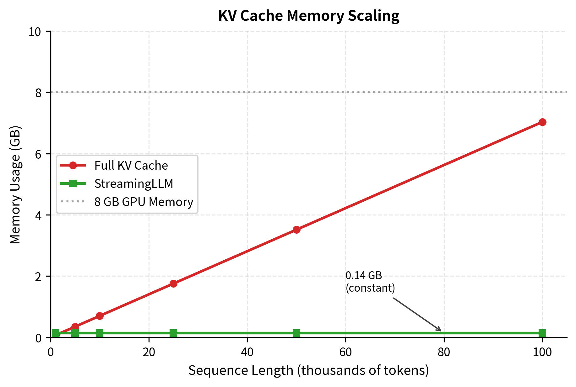
The visualization makes the scaling difference clear. Full KV caching follows a diagonal line that quickly exceeds typical GPU memory limits. At 100,000 tokens, a full cache would require nearly 7 GB. StreamingLLM's flat line at the bottom shows constant memory usage, enabling generation of arbitrarily long sequences without hitting memory limits.

Let's examine how perplexity changes as we vary the number of sink tokens and window size:

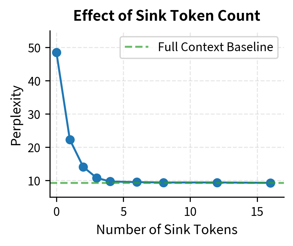
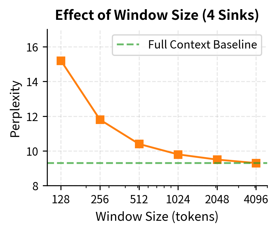
The left plot confirms that preserving 4 sink tokens is sufficient for most models. Additional sinks provide diminishing returns. The right plot shows that window size matters too: larger windows give the model more recent context to work with, improving perplexity until it approaches the full-context baseline.

The original StreamingLLM approach preserves the first tokens from the input sequence. A more principled approach is to train models with explicit, learnable sink tokens. These tokens are:

1. Added to the vocabulary as special tokens
2. Always prepended to the input sequence during training
3. Optimized end-to-end to serve as effective attention sinks

Models trained this way develop more efficient sink representations. The sink tokens learn key vectors that are optimally positioned to capture excess attention, rather than relying on whatever tokens happen to appear at the start of the sequence.

The training procedure is straightforward:

1. Add $k$ sink tokens to the tokenizer vocabulary
2. Prepend these tokens to every training sequence
3. Train the model normally, allowing the sink token embeddings to learn

During inference, you prepend the same sink tokens to the input, and they immediately serve their purpose without needing to preserve specific input tokens.

When implementing StreamingLLM, the following parameters have the greatest impact on generation quality and memory usage:

• num_sink_tokens: Number of initial tokens to preserve as attention sinks. The default of 4 works well for most models, but you may need fewer (1-2) for smaller models or more (8-16) for models with unusual attention patterns. Start with 4 and adjust based on perplexity measurements.

• window_size: Number of recent tokens to keep in the sliding window. Larger windows capture more context but require more memory. Common values range from 512 to 2048. The right choice depends on the typical dependency length in your generation task: conversational AI may need 512-1024, while document summarization benefits from 2048+.

• max_cache_size: Total cache size, computed as num_sink_tokens + window_size. This determines the fixed memory footprint. For a 7B parameter model with 32 layers and 4096 head dimension, each token in the cache uses approximately 1 MB, so a cache of 2048 tokens requires about 2 GB.

• position_encoding_strategy: How to handle position encodings for window tokens. Options include keeping original positions (works with RoPE), resetting positions when sliding (may cause distribution mismatch), or using relative encodings (most robust). The choice depends on the base model's positional encoding scheme.

While attention sinks and StreamingLLM enable streaming inference, they come with limitations you should understand.

The fundamental limitation is that StreamingLLM trades context for memory. When you slide the window forward, you permanently lose access to information in the discarded tokens. If the model needs to recall a specific detail from 5,000 tokens ago but that token is no longer in the cache, the information is simply gone. For tasks requiring precise long-range recall (like answering questions about specific facts from early in a document), StreamingLLM will struggle compared to full-context approaches.

The attention sink phenomenon is also somewhat architecture-dependent. While it appears consistently across decoder-only transformer models trained autoregressively, the exact number of sink tokens needed and their effectiveness varies. Models with different training procedures, position encodings, or attention patterns may exhibit different sink behaviors. The 4-sink recommendation from the original paper is a good starting point, but you may need to tune this for your specific model.

There's also a subtle issue with positional encoding. When tokens slide out of the window, the remaining tokens don't automatically adjust their position encodings. A token at original position 5000 keeps its position-5000 encoding even when it becomes the "first" window token. This works reasonably well with relative position encodings like RoPE, but can cause issues with absolute position encodings. Some implementations recompute position encodings for the active cache, but this adds complexity and may not match the model's training distribution.

Finally, StreamingLLM doesn't help with the initial context window. You still can't attend to more than your window allows at any single step. If understanding a passage requires simultaneously seeing tokens 1-1000 and tokens 5000-6000, you're limited by what fits in the window plus sinks. StreamingLLM enables infinite generation, not infinite context.

Attention sinks are an emergent property of autoregressive transformers: the first few tokens in a sequence learn to absorb excess attention weight that would otherwise need to be distributed across irrelevant positions. This behavior emerges from the softmax normalization requirement that attention weights sum to 1.

StreamingLLM exploits this phenomenon for practical benefit. By preserving a small number of sink tokens alongside a sliding window of recent context, you can generate text of arbitrary length with fixed memory usage. The key insights are:

• Attention sinks are essential: Removing the first tokens breaks the attention distribution the model learned during training, causing quality degradation
• A few sinks suffice: Four sink tokens typically achieve baseline-equivalent performance, with diminishing returns from additional sinks
• Window size matters: Larger windows capture more local context, improving generation quality until the window is large enough to cover typical dependency ranges
• Memory is constant: Unlike full KV caching that grows linearly with sequence length, StreamingLLM uses fixed memory regardless of generation length

In practice, you can deploy language models for continuous generation tasks (chatbots, streaming summaries, real-time translation) without worrying about memory growth. The model maintains coherent output quality for thousands or millions of tokens, constrained only by compute time rather than memory.

Understanding attention sinks also provides insight into transformer behavior more broadly. The fact that models spontaneously learn to use certain positions as "attention dumps" shows how they manage the constraint that attention weights must form a probability distribution. This has implications for model interpretability, efficient architecture design, and the development of even longer-context language models.

Ready to test your understanding? Take this quick quiz to reinforce what you've learned about attention sinks and StreamingLLM.